Appendix A: Foundations of Vector Analysis and Partial Differential Equations
Story so far:
In the main text, we have been introducing step by step the mathematical tools needed to understand general relativity. Tensors, covariant derivatives, the curvature tensor—all the language for describing curved spacetime was a generalization of "vector analysis in flat space." In this appendix, we organize the fundamental formulas of vector analysis in 3-dimensional Euclidean space, complete with proofs, which formed the foundation of the main text.
Goals of this chapter
- Provide a self-contained summary, from definitions to proofs, of the partial derivatives, vector products (cross products), differential operators (grad, div, curl, Laplacian), and integral theorems (Gauss's theorem, Stokes' theorem) that we used as "known" throughout the main text
- Consolidate in one place the mathematical tools used throughout the main text and the subsequent volumes on quantum mechanics, quantum field theory, and string theory
🟡 Lina: This appendix gathers in one place all the tools we repeatedly referenced in the main text with phrases like "in the 3-dimensional case, it was like this." Almost no new concepts appear here, so feel free to use it like a dictionary. It will also be referenced from the quantum mechanics, quantum field theory, and string theory volumes as the foundation for partial derivatives and grad/div/curl.
🔵 Kai: Honestly, there were moments during the main text when you'd say something like "from the antisymmetry of the vector product..." and I felt a bit uncertain. It's a relief to be able to check things here.
⚪ Mei: I want to verify the details of the proofs. Especially around the relationship between the scalar triple product and determinants.
🟡 Lina: Then let's go in order. Starting with partial derivatives—since we'll use these in quantum mechanics and quantum field theory as well, let's organize them properly.
A.0: Partial Derivatives — Rates of Change for Multivariable Functions
Why We Need Partial Derivatives
🟡 Lina: High school calculus deals with single-variable functions \(f(x)\). But in physics, functions that depend on multiple variables appear all the time—gravitational potential \(\Phi(x, y, z)\), the electric field \(\mathbf{E}(x, y, z, t)\), the metric tensor \(g_{\mu\nu}(x)\).
🔵 Kai: When I want to know "how much it changes in the \(x\) direction," what do I do with the other variables?
🟡 Lina: Hold them fixed. That's all.
Definition of Partial Derivatives
Recall the derivative of a single-variable function \(f(x)\):
This is the ratio of "how much \(f\) changes when \(x\) changes slightly"—the slope of the function. For a multivariable function \(f(x, y, z)\), we "differentiate with respect to \(x\) only, holding \(y\) and \(z\) fixed":
The only change is that the symbol switches from \(d\) to \(\partial\) (read "round d" or "partial"), and what you're doing is the same as ordinary differentiation. You just differentiate with respect to one variable while treating the others as constants.
Worked Examples
🟡 Lina: Let's actually do this. When \(f(x, y) = x^2 y + 3xy^2\):
\(\partial f / \partial x\) (treating \(y\) as a constant):
Combined: \(\partial f/\partial x = 2xy + 3y^2\).
\(\partial f / \partial y\) (treating \(x\) as a constant):
Combined: \(\partial f/\partial y = x^2 + 6xy\).
🔵 Kai: So it's the same calculation as ordinary differentiation, just treating the other letters as constants.
Second-Order Partial Derivatives and Schwarz's Theorem
Taking the partial derivative of a partial derivative:
Mixed partial derivatives (differentiating twice with respect to different variables):
Let's verify with our earlier example: differentiating \(\partial f/\partial y = x^2 + 6xy\) with respect to \(x\) gives \(\partial^2 f/(\partial x \partial y) = 2x + 6y\). Doing it in the reverse order—differentiating \(\partial f/\partial x = 2xy + 3y^2\) with respect to \(y\)—also gives \(2x + 6y\).
⚪ Mei: The result is the same regardless of the order!
🟡 Lina: For typical (sufficiently smooth) functions, the result is the same regardless of the order of differentiation:
This is called Schwarz's theorem (symmetry of mixed partials). In the main text, we always assume this holds. This property is used everywhere—when showing \(\operatorname{rot}(\operatorname{grad}\varphi) = 0\) or the symmetry of Christoffel symbols.
🔵 Kai: This doesn't hold for just any function, right? What exactly does "sufficiently smooth" mean as a condition?
🟡 Lina: It holds as long as the second-order mixed partial derivatives are continuous—functions encountered in physics normally satisfy this condition, so in practice you can always use it.
✅ Comprehension Check: What is Schwarz's theorem?
Answer
For sufficiently smooth functions, the order of mixed partial derivatives can be interchanged without changing the result: \(\partial^2 f/(\partial x \partial y) = \partial^2 f/(\partial y \partial x)\).
Multivariable Chain Rule
🟡 Lina: Let's extend the chain rule you learned in high school, \(\frac{d}{dx}f(g(x)) = f'(g(x))\cdot g'(x)\), to multiple variables.
For \(f(x, y)\), where \(x\) and \(y\) are each functions of a parameter \(t\): \(x = x(t)\), \(y = y(t)\):
Derivation: When \(t\) changes by \(\Delta t\), \(x\) changes by \(\Delta x = (dx/dt)\Delta t\) and \(y\) changes by \(\Delta y = (dy/dt)\Delta t\). The change in \(f\) is obtained by applying the single-variable approximation "\(\Delta f \approx f'(x)\Delta x\)" to each variable and adding them up:
Why can we simply add them? Because terms like \(\Delta x \cdot \Delta y\)—products of two infinitesimal quantities—approach zero faster than the individual \(\Delta x\) and \(\Delta y\) terms as \(\Delta t \to 0\), so they can be ignored. Dividing by \(\Delta t\) and taking the limit \(\Delta t \to 0\) gives the formula above.
🔵 Kai: This is what you use when tracking the time evolution of an electromagnetic wave's phase \(\phi(x, t) = kx - \omega t\), right?
🟡 Lina: Exactly. The chain rule plays an essential role in the d'Alembert solution of the wave equation and in the derivation of the geodesic equation in the main text.
Total Differential
Writing the chain rule in the form "before dividing by \(dt\)" gives us the total differential:
"The infinitesimal change in \(f\) is the sum of the products of each partial derivative and the corresponding infinitesimal displacement." This expression leads to the derivation of the gradient in A.4.
✅ Comprehension Check: When computing the partial derivative \(\partial f/\partial x\), how do you treat \(y\) and \(z\)?
Answer
Treat them as constants and differentiate with respect to \(x\) only.
A.1: Vector Product (Cross Product)
Definition
🟡 Lina: We want to represent "the area and orientation of the parallelogram spanned by two vectors" as a single vector—that's the motivation for defining the vector product (cross product). The vector product \(\boldsymbol{a} \times \boldsymbol{b}\) of 3-dimensional vectors \(\boldsymbol{a} = (a_1,\, a_2,\, a_3)\) and \(\boldsymbol{b} = (b_1,\, b_2,\, b_3)\) is defined as:
🔵 Kai: The dot product gives a scalar as the result, but the cross product gives a vector, right?
🟡 Lina: Yes. And this operation is defined only in 3 dimensions. It can't be used in this form in 2 or 4 dimensions. When we moved to arbitrary dimensions in the main text, the reason we used antisymmetrization of tensors instead of cross products was precisely to overcome this limitation.
✅ Comprehension Check: In how many dimensions can the vector product (cross product) be defined? Also, how was this limitation overcome in the main text?
Answer
The vector product in its standard form is defined only in 3 dimensions. In the main text, antisymmetrization of tensors was used to generalize it to arbitrary dimensions.
🟡 Lina: As a way to remember it, there's a method using a formal determinant. First, let me explain what a determinant is. For a \(2 \times 2\) array of numbers (matrix) \(\begin{pmatrix} a & b \\ c & d \end{pmatrix}\), the operation that assigns the single number \(ad - bc\) (the difference of diagonal products) is called the \(2 \times 2\) determinant, written as \(\begin{vmatrix} a & b \\ c & d \end{vmatrix} = ad - bc\). For the \(3 \times 3\) case, let's first see the procedure on a concrete example and then generalize. Using the standard basis \(\boldsymbol{e}_1 = (1,0,0)\), \(\boldsymbol{e}_2 = (0,1,0)\), \(\boldsymbol{e}_3 = (0,0,1)\):
🔵 Kai: The expansion procedure for determinants seems a bit complicated.
🟡 Lina: Let's actually do it. You expand along the first row, assigning alternating signs \(+, -, +\) to each element (this sign pattern comes from the definition of the determinant—remember it as a "checkerboard pattern" where the top-left is \(+\) and the sign flips with each step). First, the \(\boldsymbol{e}_1\) term: removing the first row and first column containing \(\boldsymbol{e}_1\) leaves \(\begin{vmatrix} a_2 & a_3 \\ b_2 & b_3 \end{vmatrix} = a_2 b_3 - a_3 b_2\). Sign is \(+\). Next, the \(\boldsymbol{e}_2\) term: removing the first row and second column gives \(\begin{vmatrix} a_1 & a_3 \\ b_1 & b_3 \end{vmatrix} = a_1 b_3 - a_3 b_1\). Sign is \(-\). Finally, the \(\boldsymbol{e}_3\) term: removing the first row and third column gives \(\begin{vmatrix} a_1 & a_2 \\ b_1 & b_2 \end{vmatrix} = a_1 b_2 - a_2 b_1\). Sign is \(+\). Combined:
This matches the definition. Since the first row contains vectors, it's not a strict determinant, but as a computational procedure it's very convenient.
⚪ Mei: So once you memorize the "expansion procedure for a \(3 \times 3\) determinant," you can write down the cross product components without mistakes.
📝 Exercises:
- Cross product component calculation → Problem B-1. Component Calculation of the Cross Product, orthogonality verification → Problem B-2. Orthogonality of the Cross Product
Algebraic Rules
🟡 Lina: The vector product satisfies the following rules:
🔵 Kai: The dot product is commutative—\(\boldsymbol{a} \cdot \boldsymbol{b} = \boldsymbol{b} \cdot \boldsymbol{a}\)—but the cross product picks up a sign change when you swap the order.
🟡 Lina: Yes. This "antisymmetry" is the prototype of the antisymmetric tensors that appeared repeatedly in the main text. The fact that each component of \(\operatorname{rot}\) (curl) takes the form of a "difference" also originates here.
⚪ Mei: Distributivity holds, but commutativity becomes "anti." What about associativity?
🟡 Lina: In general, \(\boldsymbol{a} \times (\boldsymbol{b} \times \boldsymbol{c}) \neq (\boldsymbol{a} \times \boldsymbol{b}) \times \boldsymbol{c}\). Associativity does not hold. This is the background for the BAC-CAB formula that comes later.
Geometric Properties
🟡 Lina: Let me summarize the geometric meaning of the vector product in three points.
(1) \(\boldsymbol{a} \times \boldsymbol{a} = \boldsymbol{0}\)
(2) \(\boldsymbol{a} \times \boldsymbol{b}\) is perpendicular to both \(\boldsymbol{a}\) and \(\boldsymbol{b}\)
(3) \(|\boldsymbol{a} \times \boldsymbol{b}|\) equals the area of the parallelogram spanned by \(\boldsymbol{a}\) and \(\boldsymbol{b}\)
🔵 Kai: (1) follows from anticommutativity, right? \(\boldsymbol{a} \times \boldsymbol{a} = -(\boldsymbol{a} \times \boldsymbol{a})\), so \(2(\boldsymbol{a} \times \boldsymbol{a}) = \boldsymbol{0}\).
🟡 Lina: Exactly. For (2), the most reliable way is to verify it by computing the dot product.
Expanding: \(a_1 a_2 b_3 - a_1 a_3 b_2 + a_2 a_3 b_1 - a_1 a_2 b_3 + a_1 a_3 b_2 - a_2 a_3 b_1 = 0\). Each term cancels in pairs with a sign change.
⚪ Mei: I see—\(a_1 a_2 b_3\) and \(-a_1 a_2 b_3\) always have a cancellation partner.
🟡 Lina: \((\boldsymbol{a} \times \boldsymbol{b}) \cdot \boldsymbol{b} = 0\) follows similarly. So \(\boldsymbol{a} \times \boldsymbol{b}\) points in a direction perpendicular to the plane determined by \(\boldsymbol{a}\) and \(\boldsymbol{b}\). The orientation is determined by the "right-hand rule."
🟡 Lina: The proof of (3) requires a bit of calculation, but it yields an important identity. Let \(\theta\) be the angle between \(\boldsymbol{a}\) and \(\boldsymbol{b}\). The area of the parallelogram is:
Therefore:
🔵 Kai: Here you replaced \(|\boldsymbol{a}||\boldsymbol{b}|\cos\theta\) with the dot product \(\boldsymbol{a} \cdot \boldsymbol{b}\).
🟡 Lina: On the other hand, computing \(|\boldsymbol{a} \times \boldsymbol{b}|^2\) in components:
Expanding this and confirming it equals \((a_1^2 + a_2^2 + a_3^2)(b_1^2 + b_2^2 + b_3^2) - (a_1 b_1 + a_2 b_2 + a_3 b_3)^2\) completes the proof. The resulting identity:
is called the Lagrange identity.
🔵 Kai: So the square of the dot product plus the square of the cross product equals the square of the product of magnitudes. It's a reflection of \(\cos^2\theta + \sin^2\theta = 1\).
🟡 Lina: Exactly. Beautiful, isn't it?
✅ Comprehension Check: State the geometric meaning of the vector product \(\boldsymbol{a} \times \boldsymbol{b}\).
Answer
It is a vector perpendicular to the parallelogram spanned by \(\boldsymbol{a}\) and \(\boldsymbol{b}\), with magnitude equal to the area of that parallelogram, \(|\boldsymbol{a}||\boldsymbol{b}|\sin\theta\). Its direction is determined by the right-hand rule.
A.2: Scalar Triple Product
🟡 Lina: There is a quantity formed from three vectors \(\boldsymbol{a}\), \(\boldsymbol{b}\), \(\boldsymbol{c}\) with the following property:
This quantity is called the scalar triple product.
🔵 Kai: The value doesn't change even if you cyclically permute them (\(\boldsymbol{a} \to \boldsymbol{b} \to \boldsymbol{c} \to \boldsymbol{a}\))?
🟡 Lina: That's right. The proof is straightforward—just write out the components directly.
⚪ Mei: Expanding gives 6 terms: \(a_1 b_2 c_3 - a_1 b_3 c_2 + a_2 b_3 c_1 - a_2 b_1 c_3 + a_3 b_1 c_2 - a_3 b_2 c_1\). Every term has the indices \(1, 2, 3\) distributed one each among \(a\), \(b\), \(c\).
🔵 Kai: Does cyclically permuting these really give the same result?
🟡 Lina: Try it. Substituting \(a \to b,\, b \to c,\, c \to a\) gives \(b_1 c_2 a_3 - b_1 c_3 a_2 + \cdots\)—rearranging gives the same collection of 6 terms. Writing it as a determinant makes the structure even clearer:
Determinants have the property that "swapping two rows flips the sign" (you can verify this in the \(2 \times 2\) case: \(\begin{vmatrix} c & d \\ a & b \end{vmatrix} = cb - da = -(ad - bc) = -\begin{vmatrix} a & b \\ c & d \end{vmatrix}\). For \(3 \times 3\) you can verify it via cofactor expansion, but here we'll accept and use the result). A cyclic permutation \((1 \to 2 \to 3 \to 1)\) can be achieved by 2 row swaps (for example, 1↔2 followed by 2↔3), so the sign changes by \((-1)^2 = +1\)—meaning the value doesn't change. This is the origin of the cyclic symmetry of the scalar triple product.
🔵 Kai: What does it mean geometrically?
🟡 Lina: It's the signed volume of the parallelepiped spanned by \(\boldsymbol{a}\), \(\boldsymbol{b}\), \(\boldsymbol{c}\). \(\boldsymbol{b} \times \boldsymbol{c}\) is a vector perpendicular to the base (the parallelogram of \(\boldsymbol{b}\) and \(\boldsymbol{c}\)) with magnitude equal to the base area. Taking its dot product with \(\boldsymbol{a}\) gives base area \(\times\) height \(=\) volume. Looking at Fig. A.1 "Scalar triple product and parallelepiped volume", you can clearly see this structure.
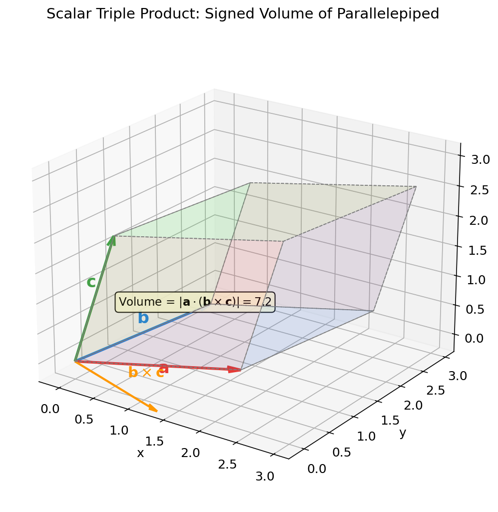
Fig. A.1: Scalar triple product and parallelepiped volume. The scalar triple product \(\boldsymbol{a} \cdot (\boldsymbol{b} \times \boldsymbol{c})\) equals the signed volume of the parallelepiped spanned by the three vectors. \(\boldsymbol{b} \times \boldsymbol{c}\) (orange) is perpendicular to the base with magnitude equal to the base area. Its dot product with \(\boldsymbol{a}\) gives the volume.
⚪ Mei: If the sign is positive, \(\boldsymbol{a}\), \(\boldsymbol{b}\), \(\boldsymbol{c}\) form a right-handed system; if negative, a left-handed system.
✅ Comprehension Check: What is the geometric meaning of the scalar triple product \(\boldsymbol{a} \cdot (\boldsymbol{b} \times \boldsymbol{c})\)? Also, what property does it have under cyclic permutation?
Answer
It represents the signed volume of the parallelepiped spanned by the three vectors. Under cyclic permutation \(\boldsymbol{a} \to \boldsymbol{b} \to \boldsymbol{c} \to \boldsymbol{a}\), the value remains unchanged (cyclic symmetry).
📝 Exercises:
- Determinant calculation of scalar triple product → Problem B-3. Scalar Triple Product
A.3: Dot Product of Two Cross Products (Prelude to the BAC-CAB Formula)
🟡 Lina: When we discussed the geometric meaning of the curvature tensor in the main text, we used the following formula. For four vectors \(\boldsymbol{a}\), \(\boldsymbol{b}\), \(\boldsymbol{c}\), \(\boldsymbol{d}\):
🔵 Kai: The right-hand side looks like a determinant.
🟡 Lina: It can also be written as a \(2 \times 2\) determinant:
⚪ Mei: The difference of diagonal products: \((\boldsymbol{a} \cdot \boldsymbol{c})(\boldsymbol{b} \cdot \boldsymbol{d}) - (\boldsymbol{a} \cdot \boldsymbol{d})(\boldsymbol{b} \cdot \boldsymbol{c})\).
🟡 Lina: The proof has a clear structure when using the scalar triple product. Treating \(\boldsymbol{c} \times \boldsymbol{d}\) as a single vector \(\boldsymbol{e}\), the cyclic symmetry of the scalar triple product from A.2 gives:
So \((\boldsymbol{a} \times \boldsymbol{b}) \cdot (\boldsymbol{c} \times \boldsymbol{d}) = \boldsymbol{a} \cdot [\boldsymbol{b} \times (\boldsymbol{c} \times \boldsymbol{d})]\).
Here we use the BAC-CAB formula (vector triple product formula). This formula can be proved directly by component calculation (see exercise Problem M-1. Proof of the BAC-CAB Formula for the proof):
Using this:
🔵 Kai: So it has the name BAC-CAB. But the current formula is \(\boldsymbol{b} \times (\boldsymbol{c} \times \boldsymbol{d})\), so the letters are different...
🟡 Lina: Historically, you memorize it in the form \(\boldsymbol{a} \times (\boldsymbol{b} \times \boldsymbol{c}) = \boldsymbol{b}(\boldsymbol{a} \cdot \boldsymbol{c}) - \boldsymbol{c}(\boldsymbol{a} \cdot \boldsymbol{b})\) as "BAC minus CAB." Read the first letters of the right-hand side: B-A-C minus C-A-B. It's the same structure with just relabeled variables.
🔵 Kai: I see, so the "outer" vector enters the "middle" to form a dot product pattern. But why is the result a linear combination of \(\boldsymbol{b}\) and \(\boldsymbol{c}\)? Doesn't any component in the \(\boldsymbol{a}\) direction appear?
🟡 Lina: Good question. \(\boldsymbol{b} \times \boldsymbol{c}\) is a vector perpendicular to the plane spanned by \(\boldsymbol{b}\) and \(\boldsymbol{c}\), right? Taking the cross product of that with \(\boldsymbol{a}\) gives a result perpendicular to \(\boldsymbol{b} \times \boldsymbol{c}\)—meaning it comes back into the plane spanned by \(\boldsymbol{b}\) and \(\boldsymbol{c}\). A vector in that plane can be written as a linear combination of \(\boldsymbol{b}\) and \(\boldsymbol{c}\), which span it. That's why no component in the \(\boldsymbol{a}\) direction appears.
⚪ Mei: Something geometrically obvious is properly reflected in the form of the formula.
✅ Comprehension Check: In the BAC-CAB formula \(\boldsymbol{a} \times (\boldsymbol{b} \times \boldsymbol{c}) = \boldsymbol{b}(\boldsymbol{a} \cdot \boldsymbol{c}) - \boldsymbol{c}(\boldsymbol{a} \cdot \boldsymbol{b})\), in what form is the vector triple product expressed?
Answer
It is expressed as a linear combination of the two vectors \(\boldsymbol{b}\), \(\boldsymbol{c}\) inside the cross product. The coefficients are determined by dot products with the outer vector \(\boldsymbol{a}\).
📝 Exercises:
- Numerical verification of Lagrange's identity → Problem B-8. Verification of the Lagrange Identity, numerical verification of BAC-CAB formula → Problem B-9. Verification of the BAC-CAB Formula, general proof of BAC-CAB formula → Problem M-1. Proof of the BAC-CAB Formula, dot product of two cross products → Problem M-3. Inner Product of Two Cross Products Formula, unified derivation via Levi-Civita symbol → Problem A-1. Identities Using the Levi-Civita Symbol
A.4: Differential Operators
🟡 Lina: From here, we define differential operations on vector fields and scalar fields. These are the "flat space versions" of the covariant derivative that we generalized to curved spacetime in the main text.
The Nabla Operator
🟡 Lina: First, let me introduce the nabla operator \(\nabla\), which is the parent of all differential operators. In 3-dimensional Cartesian coordinates \((x, y, z)\):
Think of this as a "differential operator that behaves like a vector."
🔵 Kai: A vector whose components are partial derivatives...?
🟡 Lina: Yes, that's why it's an "operator." By itself it has no meaning—it only becomes meaningful when it acts on something. Acting on a scalar field gives grad, taking the dot product with a vector field gives div, and taking the cross product with a vector field gives curl.
Gradient
🟡 Lina: Acting with \(\nabla\) on a scalar field \(\varphi(x, y, z)\):
⚪ Mei: The result is a vector field. You input a scalar and get out a vector.
🟡 Lina: Yes. And physically, \(\nabla\varphi\) points in "the direction in which \(\varphi\) increases most rapidly," and its magnitude gives "the maximum rate of change." Each component \(\partial\varphi/\partial x\), etc., represents the rate of change in that direction. You remember how we derived the gravitational field \(\boldsymbol{g} = -\nabla\varphi\) from the gravitational potential \(\varphi\) in the main text.
Divergence
🟡 Lina: For a vector field \(\boldsymbol{F} = (F_x,\, F_y,\, F_z)\), taking the "dot product" with \(\nabla\):
🔵 Kai: The result is a scalar.
🟡 Lina: Yes. Physically, it represents "how much the vector field is flowing out from that point." \(\operatorname{div}\boldsymbol{F} > 0\) means a source, \(< 0\) means a sink. Maxwell's equation \(\operatorname{div}\boldsymbol{E} = \rho/\varepsilon_0\) meant "the electric field flows out from locations where charge density \(\rho\) exists."
Derivation from an Infinitesimal Volume
🟡 Lina: Let's derive why this sum of partial derivatives represents "outflow" from a physical picture.
Consider a tiny rectangular box centered at \((x_0, y_0, z_0)\) with sides \(\Delta x\), \(\Delta y\), \(\Delta z\) (imagine examining how much \(\boldsymbol{F}\) flows out or in through each face—we consider 3 pairs: right and left faces, top and bottom faces, front and back faces). We'll calculate the net outflow of the vector field \(\boldsymbol{F}\) from this box. In Fig. A.2 "Derivation of divergence from an infinitesimal volume", I've drawn the flow of \(F_x\) through the right and left faces as an example for the \(x\) direction—read along while looking at it (the \(y\) and \(z\) directions follow the same approach).
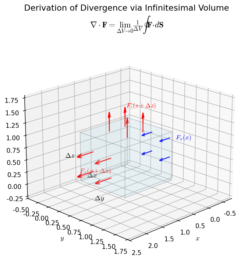
Fig. A.2: Derivation of divergence from an infinitesimal volume. Flow of the vector field through each face of an infinitesimal rectangular box centered at \((x_0, y_0, z_0)\). The difference in \(F_x\) between the right and left faces gives the net outflow in the \(x\) direction.
Net outflow in the \(x\) direction: Subtract the amount entering through the left face (\(x_0 - \Delta x/2\)) from the amount exiting through the right face (\(x_0 + \Delta x/2\)):
🔵 Kai: You subtract what comes in through the left face from what goes out through the right face.
🟡 Lina: Exactly. We use a first-order approximation of \(F_x\) around \(x_0\). Rearranging the definition of the partial derivative \(\partial F_x/\partial x = \lim_{h\to 0}[F_x(x_0+h) - F_x(x_0)]/h\), for sufficiently small \(h\) we get the approximation \(F_x(x_0 + h) \approx F_x(x_0) + (\partial F_x/\partial x)\cdot h\) (this technique of "approximating a function using its derivative" is generally called a Taylor expansion—in A.7 where we derive Euler's formula, I'll explain the general idea of Taylor expansion in detail). Using this: \(F_x(x_0 \pm \Delta x/2) \approx F_x(x_0) \pm (\partial F_x/\partial x)(\Delta x/2)\). Taking the difference gives \((\partial F_x/\partial x)\Delta x\). Therefore the net outflow in the \(x\) direction is \((\partial F_x/\partial x)\,\Delta V\) (where \(\Delta V = \Delta x \Delta y \Delta z\)).
The \(y\) and \(z\) directions are similar. The net outflow per unit volume from all 3 directions combined is the divergence:
Here, "net outflow through the closed surface" written mathematically is \(\oint_S \boldsymbol{F} \cdot d\boldsymbol{S}\). Since this may be new notation, let me explain.
🔵 Kai: How is \(\oint\) different from the regular integral sign \(\int\)?
🟡 Lina: \(\oint\) is an integral sign representing summation over an entire closed surface (or curve)—it's a regular \(\int\) with a circle on it. And \(d\boldsymbol{S}\) is the area vector of each infinitesimal surface element—a vector pointing perpendicular to the surface with magnitude equal to the area of that tiny patch. The direction perpendicular to the surface is called the normal direction—just as in high school the "tangent" was the direction along a curve, the "normal" is the direction sticking out from the surface. The convention is to take the "outward" direction—from inside to outside of the closed surface (a surface closed like a balloon). This way, a positive dot product \(\boldsymbol{F} \cdot d\boldsymbol{S}\) represents outflow, and negative represents inflow.
🔵 Kai: Is a surface integral like the high school integral of "adding up strips," but done over a surface?
🟡 Lina: Exactly that image. In high school, a definite integral "adds up strips under a curve"—summing along one dimension. A surface integral "divides the surface into tiny tiles, computes the normal component of \(\boldsymbol{F}\) times the tile area for each tile, and sums over all tiles"—summing over a 2-dimensional surface. Same idea, just one dimension higher.
🔵 Kai: The "normal component" is the component perpendicular to the surface, right? But how do you extract it?
🟡 Lina: Using the dot product. Since \(d\boldsymbol{S}\) is an area vector pointing perpendicular to the surface, the dot product \(\boldsymbol{F} \cdot d\boldsymbol{S} = |\boldsymbol{F}||d\boldsymbol{S}|\cos\alpha\) (where \(\alpha\) is the angle between \(\boldsymbol{F}\) and \(d\boldsymbol{S}\)) automatically picks out \(|\boldsymbol{F}|\cos\alpha\) = the normal component. That's the surface integral. And the relationship between this "local sum of partial derivatives" and "outflow through a closed surface," extended to a finite volume, becomes Gauss's theorem in A.6.
⚪ Mei: So the "limit of outflow through a closed surface divided by the volume" is the definition in terms of meaning, and the "sum of partial derivatives" derived from it is the formula used for actual calculations.
✅ Comprehension Check: How is the divergence \(\nabla \cdot \boldsymbol{F}\) physically defined using an infinitesimal volume?
Answer
It is defined as the limit of the net outflow of the vector field through an infinitesimal closed surface surrounding a point, divided by that infinitesimal volume. Positive means a source, negative means a sink.
Curl (Rotation)
🟡 Lina: For a vector field \(\boldsymbol{F}\), taking the "cross product" with \(\nabla\):
In components:
🔵 Kai: Each component is a "difference." So that comes from the antisymmetry of the cross product.
🟡 Lina: Exactly. Physically, it represents "how much the vector field is swirling around that point." \(\operatorname{rot}\boldsymbol{B} = \mu_0 \boldsymbol{j}\) means "the magnetic field swirls around locations where current flows."
Derivation from an Infinitesimal Loop
🟡 Lina: Just as we derived divergence from "outflow from an infinitesimal volume," the curl can be derived as "circulation around an infinitesimal loop."
Consider a tiny rectangular loop in the \(xy\) plane (center \((x_0, y_0, z_0)\), sides \(\Delta x\), \(\Delta y\)) traversed counterclockwise. For each side, compute "the component of \(\boldsymbol{F}\) along the side \(\times\) the side length," and the sum over one complete circuit is called the circulation—it's called this because you "circulate" around the loop. The key point is that the difference between contributions from opposite sides (top and bottom, right and left) gives the components of the curl. In Fig. A.3 "Derivation of curl from an infinitesimal loop", I've drawn the relationship between the sides of the infinitesimal loop and the components of \(\boldsymbol{F}\)—read along while looking at it.
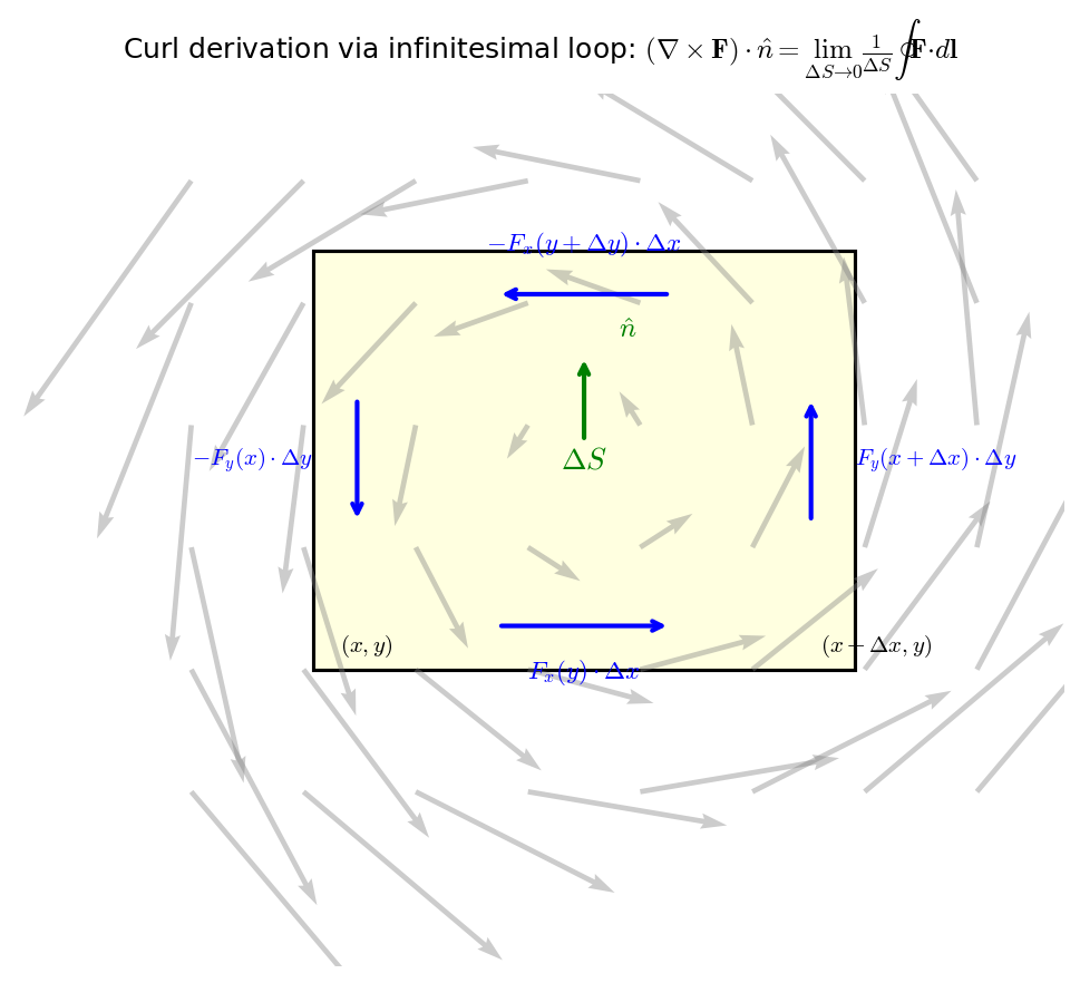
Fig. A.3: Derivation of curl from an infinitesimal loop. Traversing a tiny rectangular loop in the \(xy\) plane counterclockwise. The sum of the components of \(\boldsymbol{F}\) along the direction of travel on each side (the circulation), expressed as differences between opposite sides, gives the components of the curl.
Formally, this is written as the line integral \(\oint \boldsymbol{F} \cdot d\boldsymbol{r}\). A line integral is the operation of "dividing a curve into small segments, computing \(\boldsymbol{F}\)'s component along the direction of travel \(\times\) the segment length for each segment, and summing over all segments"—the same approach as a high school definite integral "adding strips along the \(x\)-axis," but summing along an arbitrary curve. \(d\boldsymbol{r}\) is the infinitesimal displacement vector along the curve, and the dot product \(\boldsymbol{F} \cdot d\boldsymbol{r}\) means "component of \(\boldsymbol{F}\) in the direction of travel \(\times\) infinitesimal distance." However, since we have an infinitesimal loop here, computing each side separately is sufficient. Specifically:
- Bottom side (\(y = y_0 - \Delta y/2\), counterclockwise so traveling in the \(+x\) direction): \(+F_x(x_0, y_0 - \Delta y/2)\,\Delta x\)
- Top side (\(y = y_0 + \Delta y/2\), counterclockwise so traveling in the \(-x\) direction): \(-F_x(x_0, y_0 + \Delta y/2)\,\Delta x\)
- Right side (\(x = x_0 + \Delta x/2\), counterclockwise so traveling in the \(+y\) direction): \(+F_y(x_0 + \Delta x/2, y_0)\,\Delta y\)
- Left side (\(x = x_0 - \Delta x/2\), counterclockwise so traveling in the \(-y\) direction): \(-F_y(x_0 - \Delta x/2, y_0)\,\Delta y\)
Sign convention: \(+\) if the direction of travel matches the positive coordinate axis direction, \(-\) if opposite. Going counterclockwise: the bottom side goes right (\(+x\)), the right side goes up (\(+y\)), the top side goes left (\(-x\)), and the left side goes down (\(-y\)) (check the arrow directions in Fig. A.3 "Derivation of curl from an infinitesimal loop").
⚪ Mei: For divergence we looked at "flow through faces," but for curl we look at "components along the sides."
🟡 Lina: Exactly. Now let's combine the contributions from the right and left sides (sides parallel to the \(y\) direction). Using the first-order approximation (same Taylor expansion as in the divergence derivation), the difference between right and left sides is \([F_y(x_0 + \Delta x/2) - F_y(x_0 - \Delta x/2)]\,\Delta y \approx (\partial F_y/\partial x)\Delta x\,\Delta y\). Similarly, combining the contributions from the top and bottom sides (sides parallel to the \(x\) direction), the difference from bottom minus top is \(-[F_x(x_0, y_0 + \Delta y/2) - F_x(x_0, y_0 - \Delta y/2)]\,\Delta x \approx -(\partial F_x/\partial y)\Delta y\,\Delta x\). In total:
The circulation per unit area is the \(z\) component of the curl:
⚪ Mei: Doing the same thing with loops in the \(yz\) plane and \(zx\) plane gives the \(x\) and \(y\) components.
🟡 Lina: Yes. And extending this relationship between "circulation around a tiny loop" and "surface integral of the curl" to a finite surface gives Stokes' theorem in A.6.
🔵 Kai: Divergence is "net outflow from an infinitesimal volume," and curl is "circulation around an infinitesimal loop"—geometrically very clear. But divergence divides by volume, and curl divides by area—the dimensions are different, yet both are "relatives of \(\nabla\)."
🟡 Lina: Good observation. A single operator \(\nabla\), depending on whether it acts on a scalar field (grad), takes a dot product with a vector field (div), or takes a cross product (curl), produces entirely different physical quantities. The input/output types are all different—grad is "scalar → vector," div is "vector → scalar," curl is "vector → vector." In fact, using differential forms and the exterior derivative \(d\) introduced in Ch. 24, grad, div, and curl are all unified as a single operation of "applying \(d\)." But for now, being able to distinguish between the three faces of \(\nabla\) is sufficient.
⚪ Mei: I see—since the input/output types are all different, combining them incorrectly wouldn't even make sense.
🔵 Kai: Then the Laplacian \(\nabla^2\) is "take the grad, then take the div," so it uses the face of \(\nabla\) twice. Are there other combinations—like "take the div, then the grad" or "take the curl of the curl"?
🟡 Lina: Good question. "Taking the div, then the grad" is \(\nabla(\nabla \cdot \boldsymbol{F})\), which appears in the "curl of curl" formula in the next section A.5. "Taking the curl of the curl" is also addressed in A.5. Let's look at them in order.
✅ Comprehension Check: How is the \(z\) component of the curl \(\nabla \times \boldsymbol{F}\) physically defined using an infinitesimal loop?
Answer
It is defined as the limit of the circulation of the vector field (line integral) around an infinitesimal loop in the \(xy\) plane, divided by the infinitesimal area enclosed by that loop. This represents "how much the vector field is swirling around that point."
Laplacian
🟡 Lina: Applying \(\nabla\) twice is also important. For a scalar field \(\varphi\):
Some textbooks write \(\Delta\) instead of \(\nabla^2\), but in this book we use \(\nabla^2\) for the Laplacian to avoid confusion with the infinitesimal change \(\Delta x\).
⚪ Mei: Taking the grad and then taking the div—a two-step operation.
🟡 Lina: Newton's gravitational field equation \(\nabla^2\varphi = 4\pi G\rho\) means "the mass density \(\rho\) determines the curvature of the potential \(\varphi\)." This correspondence was key when we explained in the main text that the Einstein equation generalizes Newton's equation.
✅ Comprehension Check: What do you get when you apply the nabla operator \(\nabla\) to a scalar field? What do you get when you take the dot product with a vector field?
Answer
Applying it to a scalar field gives the gradient—a vector field representing the direction of steepest ascent and the rate of change. Taking the dot product with a vector field gives the divergence—a scalar field representing the strength of the source/sink.
📝 Exercises:
- Gradient calculation → Problem B-4. Gradient of a Scalar Field, divergence calculation → Problem B-5. Divergence of a Vector Field, curl calculation → Problem B-6. Curl of a Vector Field, Laplacian calculation → Problem B-7. Laplacian of a Scalar Field
A.5: Important Identities for Differential Operators
🟡 Lina: The following two identities were used repeatedly in the main text.
Identity 1: The Curl of a Gradient is Zero
🔵 Kai: I feel like I understand this intuitively... The gradient is "the direction up the slope," right? If you walk in the uphill direction, you never go around in a circle back to where you started—so there's no vortex?
🟡 Lina: Exactly. You can also verify it physically. Writing it in components, for example the \(x\) component is \(\frac{\partial^2\varphi}{\partial y\partial z} - \frac{\partial^2\varphi}{\partial z\partial y}\). If \(\varphi\) is sufficiently smooth, we can exchange the order of partial differentiation, so this is \(0\). In other words, a field derived from a potential, like the conservative force field \(\boldsymbol{F} = -\nabla\varphi\), has no vorticity.
⚪ Mei: I see—because of Schwarz's theorem from A.0, the mixed partial derivatives cancel, making each component zero.
🔵 Kai: Conversely, if \(\operatorname{rot}\boldsymbol{F} = \boldsymbol{0}\), does a potential necessarily exist?
🟡 Lina: Good question. In regions without holes—for example, the interior of a ball, where any rubber band you place can be shrunk to a point—yes, you can say that (in mathematics, such regions are called "simply connected"). Conversely, on the surface of a donut where there's a hole, a rubber band threaded through the hole can't be shrunk to a point without cutting it—along such a loop, counterexamples can be constructed where \(\operatorname{rot}\boldsymbol{F} = \boldsymbol{0}\) but the circulation isn't zero. For now, just keep this intuition. After learning Stokes' theorem in A.6, think about how "\(\operatorname{rot}\boldsymbol{F} = \boldsymbol{0}\) implies the circulation is zero along any closed curve" is derived.
🔵 Kai: I see, so as long as there are no holes, it's fine. Once I learn Stokes' theorem in A.6, it should become clearer.
Identity 2: The Divergence of a Curl is Zero
🟡 Lina: This also follows from exactly the same argument—Schwarz's theorem—as Identity 1. Expanding \(\nabla \cdot (\nabla \times \boldsymbol{F})\), for example \(\partial_x(\partial_y F_z - \partial_z F_y) + \cdots\), each term takes the form of a difference of mixed partial derivatives and all cancel. I'll leave the detailed verification as an exercise. Physically, \(\operatorname{div}\boldsymbol{B} = 0\) (magnetic monopoles don't exist) is also a consequence of \(\boldsymbol{B} = \operatorname{rot}\boldsymbol{A}\).
🔵 Kai: Identity 1 is "if there's a potential, there's no vortex," and Identity 2 is "a field born from a vortex has no source"—they're paired.
Identity 3: Curl of a Curl
🟡 Lina: This identity is decisive when deriving the electromagnetic wave equation from Maxwell's equations. Let's verify the \(x\) component.
Setting \(\nabla \times \boldsymbol{F} = \boldsymbol{B}\) and writing out the components: \(B_x = \partial_y F_z - \partial_z F_y\), \(B_y = \partial_z F_x - \partial_x F_z\), \(B_z = \partial_x F_y - \partial_y F_x\).
The \(x\) component of \(\nabla \times \boldsymbol{B}\) is \(\partial_y B_z - \partial_z B_y\). Substituting:
⚪ Mei: We use Schwarz's theorem to swap the order of differentiation and reorganize.
🟡 Lina: Exactly. Using Schwarz's theorem, \(\partial_y\partial_x = \partial_x\partial_y\) and \(\partial_z\partial_x = \partial_x\partial_z\):
To construct \(\nabla \cdot \boldsymbol{F} = \partial_x F_x + \partial_y F_y + \partial_z F_z\), we add and subtract \(\partial_x^2 F_x\) (\(+\partial_x^2 F_x - \partial_x^2 F_x = 0\) so the value doesn't change):
The \(y\) and \(z\) components work the same way, so the identity holds as a vector equation.
🔵 Kai: So if \(\nabla \cdot \boldsymbol{F} = 0\), then \(\nabla(\nabla \cdot \boldsymbol{F})\) vanishes and we get \(\nabla \times (\nabla \times \boldsymbol{F}) = -\nabla^2 \boldsymbol{F}\), leaving only the Laplacian. The electromagnetic wave equation appeared in the main text because \(\nabla \cdot \boldsymbol{E} = 0\) in regions without charge?
🟡 Lina: Exactly.
🔵 Kai: Then conversely, in regions with charge, you don't get a simple wave equation?
🟡 Lina: That's right. In regions with charge, \(\nabla \cdot \boldsymbol{E} = \rho/\varepsilon_0 \neq 0\), so the \(\nabla(\nabla \cdot \boldsymbol{E})\) term remains, and it doesn't reduce to a pure wave equation. The gradient of the charge distribution appears on the right-hand side as a "source."
⚪ Mei: So only when \(\nabla \cdot \boldsymbol{F} = 0\) does the Laplacian alone remain, giving a wave equation—whether the divergence is zero or not changes the form of the equation.
🔵 Kai: So gravitational waves also became a wave equation because it's "in vacuum"? What happens in regions with matter?
🟡 Lina: Good observation. As we discussed in ch19 of the main text, in vacuum the linearized Einstein equation becomes a wave equation and gravitational waves propagate. In regions with matter, a "source" remains on the right-hand side, and wave generation occurs—the quadrupole formula was derived precisely from this "equation with sources."
⚪ Mei: I see—whether it's vacuum or not changes the form of the equation, separating propagation from generation.
🟡 Lina: Exactly. Now, we've assembled all the important identities for differential operators. Let's move on to the integral theorems.
📝 Exercises:
- Verification of rot(grad φ) = 0 → Problem B-10. Verifying rot(grad) = 0, proof of div(rot F) = 0 → Problem M-2. Proof that div(curl) = 0, divergence product rule → Problem M-4. Product Rule for Divergence
A.6: Integral Theorems
🟡 Lina: Finally, let me state the two great theorems connecting differentiation and integration. I'll omit the proofs, but understanding the physical meaning is important.
Gauss's Theorem (Divergence Theorem)
Here \(V\) is the region enclosed by the closed surface \(S\), and \(d\boldsymbol{S}\) is the outward-pointing normal area element. The right-hand side \(\int_V \cdots dV\) is a volume integral—dividing the region \(V\) into tiny cubes, computing \(\operatorname{div}\boldsymbol{F}\) times the tiny volume \(dV\) for each cube, and summing over all cubes. While a surface integral "divides a surface into tiny tiles and sums," a volume integral "divides a solid into tiny blocks and sums"—the same idea, just one dimension higher.
🔵 Kai: The left side is "the total flow going out through the surface," the right side is "the total of all sources inside." And you're saying they're equal.
🟡 Lina: Exactly. When we discussed the physical meaning of the Einstein equation in the main text, we used an analogy with Gauss's theorem as "the relationship between local curvature (analogous to div) and the global deviation of geodesics (analogous to the surface integral)."
⚪ Mei: In A.4, "the net outflow from an infinitesimal volume divided by the volume" was the divergence, so summing that up over a finite volume gives this theorem—a bridge connecting local and global.
✅ Comprehension Check: What two quantities does Gauss's theorem (divergence theorem) state are equal?
Answer
The net outflow of the vector field through a closed surface \(S\) (the surface integral \(\oint_S \boldsymbol{F} \cdot d\boldsymbol{S}\)) equals the volume integral of the divergence over the region enclosed by that surface (\(\int_V \operatorname{div}\boldsymbol{F}\, dV\)).
Stokes' Theorem
Here \(C\) is the closed curve forming the boundary of surface \(S\), and \(d\boldsymbol{r}\) is the infinitesimal displacement vector along the curve (the same line integral notation introduced in A.4).
⚪ Mei: The left side is "the circulation along the closed curve," the right side is "the total vorticity penetrating the surface bounded by that curve."
🟡 Lina: In the main text, when we discussed the path-dependence of parallel transport (holonomy), we talked about how "the deviation when transporting a vector around a closed curve" equals "the surface integral of curvature over the enclosed surface." That was the curved-space version of Stokes' theorem.
🔵 Kai: Ah, so that's why you said "generalization of Stokes' theorem" in the main text. It comes back to here.
✅ Comprehension Check: What two quantities does Stokes' theorem state are equal?
Answer
The circulation of the vector field along a closed curve \(C\) (the line integral \(\oint_C \boldsymbol{F} \cdot d\boldsymbol{r}\)) equals the surface integral of the curl over a surface \(S\) bounded by that closed curve (\(\int_S (\operatorname{rot}\boldsymbol{F}) \cdot d\boldsymbol{S}\)).
📝 Exercises:
- Application of Gauss's theorem (Coulomb field) → Problem M-5. Gauss's Theorem and the Coulomb Electric Field, Stokes' theorem and conservative fields/curvature → Problem A-2. Applications of Stokes' Theorem
A.7: The Wave Equation — Classification of Second-Order PDEs and d'Alembert's Solution
🟡 Lina: From here, let's classify the second-order partial differential equations that appear repeatedly in the main text. In ch01, we compared the Poisson equation with the electromagnetic wave equation, and in ch19 we derived the gravitational wave equation from the linearization of the Einstein equation. In the string theory volume, the vibrations of a string also obey the wave equation. By organizing these together, we can understand the behavior of solutions with good perspective.
Why Classification is Needed
The partial differential equations encountered in physics may look similar but have completely different solution properties. Solutions to the wave equation oscillate, solutions to the diffusion equation decay, and solutions to the Poisson equation are static. By identifying the type of equation, you can predict the behavior of its solutions.
Three Types
Table A.1: Three types of second-order PDEs and their physical meaning
| Type | Standard form (1D) | Physical meaning | Chapters where it appears |
|---|---|---|---|
| Wave equation (hyperbolic) | \(\partial_t^2 f = v^2 \partial_x^2 f\) | Wave propagation. Information travels at finite speed \(v\) | Ch. 1 (electromagnetic waves), Ch. 19 (gravitational waves), string theory volume (string vibrations, covered in later volumes) |
| Diffusion equation (parabolic) | \(\partial_t f = D \partial_x^2 f\) | Heat diffusion, particle diffusion. Irreversible process | Classical example: heat conduction equation |
| Poisson/Laplace equation (elliptic) | \(\nabla^2 f = \rho\) | Static field distribution. No time dependence | ch01 (gravitational potential), electrostatics |
How to Identify the Type
- Second-order time derivative present → Wave equation (oscillating solutions)
- First-order time derivative present → Diffusion equation (decaying solutions)
- No time derivative → Poisson/Laplace equation (static solutions)
⚪ Mei: Just by looking at the "face" of the equation, you can predict the behavior of the solutions.
General Solution of the 1D Wave Equation (d'Alembert's Solution)
🟡 Lina: When we treat string vibrations in ch13 of the string theory volume, we'll use the general solution of the wave equation. Let's see the derivation via a change of variables here. Starting point:
Step 1: Change of variables. Set \(\xi = x - ct\), \(\eta = x + ct\). Inversely, \(x = (\xi + \eta)/2\), \(t = (\eta - \xi)/(2c)\).
🔵 Kai: How do you come up with this change of variables?
🟡 Lina: The wave equation should contain "right-traveling waves" and "left-traveling waves." Since \(x - ct\) is the phase of a right-traveling wave and \(x + ct\) is the phase of a left-traveling wave, using these two as new coordinates should simplify the equation.
Step 2: Transform partial derivatives using the chain rule
Using the chain rule from A.0. Since \(\xi = x - ct\), \(\eta = x + ct\), we have \(\partial\xi/\partial x = 1\), \(\partial\eta/\partial x = 1\), \(\partial\xi/\partial t = -c\), \(\partial\eta/\partial t = c\). Therefore:
⚪ Mei: The chain rule from A.0 is already being used here.
Step 3: Compute second-order derivatives
🟡 Lina: Applying \(\partial/\partial x = \partial/\partial\xi + \partial/\partial\eta\) from Step 2 once more:
Similarly, applying \(\partial/\partial t = c(-\partial/\partial\xi + \partial/\partial\eta)\) once more:
Step 4: Substitute into the wave equation. Rewriting the left and right sides of the wave equation \(\partial_t^2 u = c^2 \partial_x^2 u\) in the new variables:
- Left side: \(\partial_t^2 u = c^2(\partial_{\xi}^2 u - 2\partial_{\xi}\partial_{\eta} u + \partial_{\eta}^2 u)\)
- Right side: \(c^2 \partial_x^2 u = c^2(\partial_{\xi}^2 u + 2\partial_{\xi}\partial_{\eta} u + \partial_{\eta}^2 u)\)
Substituting into the wave equation \(\partial_t^2 u = c^2 \partial_x^2 u\), both sides have \(c^2\) as a common factor. Dividing both sides by \(c^2 \neq 0\):
Subtracting \(\partial_{\xi}^2 u + \partial_{\eta}^2 u\) from both sides, only the mixed derivative terms remain: \(-2\partial_{\xi}\partial_{\eta}u = +2\partial_{\xi}\partial_{\eta}u\). Rearranging: \(-4\partial_{\xi}\partial_{\eta}u = 0\). That is:
🔵 Kai: Wow, that complicated wave equation becomes this simple just from a change of variables!
⚪ Mei: The \(\partial_\xi^2\) and \(\partial_\eta^2\) terms all cancel, leaving only the mixed derivative.
Step 5: General solution
🟡 Lina: Integrating \(\partial^2 u/(\partial\xi\partial\eta) = 0\) with respect to \(\eta\). In the single-variable case, integrating \(df/dx = 0\) gives \(f = C\) (a constant). In the partial derivative case, "\(\eta\) is treated as a constant while everything else (i.e., \(\xi\)) is free," so integrating \(\partial(\partial u/\partial\xi)/\partial\eta = 0\) with respect to \(\eta\) gives: \(\partial u/\partial\xi\) doesn't depend on \(\eta\)—that is, \(\partial u/\partial\xi = h(\xi)\) (an arbitrary function of \(\xi\) alone).
🔵 Kai: Wait a moment. In the single-variable case, "derivative is zero → constant," right? Why does the partial derivative case give "a function of \(\xi\)" instead of "a constant"?
🟡 Lina: Good question. When integrating with respect to \(\eta\), \(\xi\) is treated as a constant, so anything that "doesn't depend on \(\eta\)" works. Think of it by analogy with the single-variable case: the solution of \(df/dx = 0\) is \(f = C\) (a constant)—something that doesn't depend on \(x\). By the same logic, the solution of \(\partial(\cdots)/\partial\eta = 0\) is "something that doesn't depend on \(\eta\)" = an arbitrary function of \(\xi\). In other words, what was "the constant of integration \(C\)" in the single-variable case gets "promoted" to "an arbitrary function of the other variable" in the partial derivative case.
⚪ Mei: I see—"it's a constant from \(\eta\)'s perspective" but "free with respect to \(\xi\)," so it becomes a function of \(\xi\).
🟡 Lina: Exactly. Next, we integrate \(\partial u/\partial\xi = h(\xi)\) with respect to \(\xi\). Treating \(\eta\) as a constant, this equation has the same form as the single-variable differential equation \(dF/dx = h(x)\), so we can integrate it the same way as an ordinary indefinite integral.
By single-variable analogy: integrating \(dF/dx = h(x)\) gives \(F(x) = \int h(x)\,dx + C\) (\(C\) is the constant of integration). In our case, integrating \(\partial u/\partial\xi = h(\xi)\) with respect to \(\xi\) gives \(u = f(\xi) + (\text{the analogue of the "constant of integration"})\). Here \(f(\xi)\) is the antiderivative of \(h(\xi)\)—\(f\) is a function of \(\xi\) alone satisfying \(df/d\xi = h(\xi)\). Since \(h\) was "an arbitrary function of \(\xi\) only," \(f\) is also "an arbitrary function of \(\xi\) only" (since \(f\) is the antiderivative of \(h\), it's a smooth function). For concrete examples: if \(h(\xi) = \xi^2\) then \(f(\xi) = \xi^3/3\), if \(h(\xi) = \sin\xi\) then \(f(\xi) = -\cos\xi\), ...as \(h\) changes so does \(f\), but both remain "functions of \(\xi\) alone."
Now what about the "constant of integration"? In the single-variable case, \(C\) was "a constant that doesn't depend on \(x\)." In the partial derivative case, it only needs to "not depend on \(\xi\)," so \(C\) gets promoted to an arbitrary function of \(\eta\): \(g(\eta)\).
In the end, \(u = f(\xi) + g(\eta)\), where both \(f\) and \(g\) are arbitrary functions. Returning to the original variables:
🔵 Kai: What are these \(f\) and \(g\) specifically? Do they have to be trigonometric functions?
🟡 Lina: \(f(x - ct)\) represents a wave traveling to the right at speed \(c\), and \(g(x + ct)\) represents a wave traveling to the left. And \(f\), \(g\) can be sinusoidal waves, pulses, or any differentiable function—they're all solutions. What specific form they take is determined by the initial conditions (the wave shape and velocity at \(t = 0\)). This is the foundation for decomposing string vibrations into left-traveling and right-traveling waves in ch13 of the string theory volume.
⚪ Mei: So once the initial conditions are determined, \(f\) and \(g\) are uniquely determined.
🔵 Kai: Even when you say "determined by initial conditions," I can't quite picture what form they take... In high school physics, waves were written with \(\sin\) or \(\cos\)—are those special cases of this general solution?
🟡 Lina: Yes. For example, choosing \(f(s) = e^{-s^2}\) (a Gaussian pulse), \(u = e^{-(x-ct)^2}\) is a bell-shaped wave traveling to the right at speed \(c\). \(\sin\) and \(\cos\) are infinitely extending sinusoidal waves, but localized waves like pulses are also solutions. The reason high school only used \(\sin\) was that periodic waves were the common context—the wave equation itself admits much more general solutions.
Plane Wave Solutions and the Dispersion Relation
🟡 Lina: Good question. Let's consider the most fundamental case within d'Alembert's general solution—the "sinusoidal wave."
First we'll organize how to write a sinusoidal wave, then introduce tools for handling it efficiently (Taylor expansion and Euler's formula), and finally substitute into the wave equation to derive the dispersion relation—three steps. These tools are essential from quantum mechanics onward, so let's derive them thoroughly here.
Consider a sinusoidal wave with wavelength \(\lambda\) (the spatial length of one wave cycle) and frequency \(\nu\) (the number of oscillations per second; in high school it's often written as \(f\), but in physics \(\nu\) (the Greek letter nu) is also commonly used). Since \(\cos\theta\) completes one full oscillation every time \(\theta\) increases by \(2\pi\): to make "one cycle per \(\lambda\) in \(x\)," set the argument of \(\cos\) to \(\theta = 2\pi x/\lambda\)—when \(x\) increases by \(\lambda\), the argument increases by \(2\pi\), giving exactly one cycle. Similarly, to make "one cycle per \(1/\nu\) in \(t\)," subtract \(2\pi\nu\, t\). This gives the sinusoidal wave as \(\cos(2\pi x/\lambda - 2\pi\nu\, t)\).
🔵 Kai: The combinations \(2\pi/\lambda\) and \(2\pi\nu\) keep appearing. Is there a shorthand?
🟡 Lina: Yes. It's convenient to define the wave number \(k = 2\pi/\lambda\) and the angular frequency \(\omega = 2\pi\nu\). Here, the phase refers to the argument of \(\cos\)—that is, the value of \(kx - \omega t\) in \(\cos(kx - \omega t)\). When the phase changes by \(2\pi\), the \(\cos\) completes one cycle and returns to its original value. \(k\) represents "how much the phase increases per meter"—the shorter the wavelength \(\lambda\), the larger \(k\). For example, if \(\lambda = 2\) m then \(k = 2\pi/2 = \pi\) rad/m, meaning the phase shifts by \(\pi\) (= half a cycle) per meter. \(\omega\) represents "how much the phase increases per second"—the larger the frequency \(\nu\), the larger \(\omega\). The factor \(2\pi\) appears in both because the phase change over one full wave cycle is \(2\pi\) radians (= 360° = one complete cycle of \(\cos\)).
⚪ Mei: Now the sinusoidal wave can be written as \(\cos(kx - \omega t)\).
🟡 Lina: Yes. And rewriting it as \(\cos[k(x - (\omega/k)t)]\) shows it has the form of d'Alembert's \(f(x - ct)\)—with \(\omega/k\) corresponding to the wave speed. Now, I want to rewrite this sinusoidal wave \(\cos(kx - \omega t)\) in a more tractable form. To do that, let's first derive the relationship between exponential and trigonometric functions.
Taylor Expansion
🟡 Lina: Here I'll introduce a tool called the Taylor expansion. This is "a method of expressing a function as an infinite sum of polynomials using the function's value, first derivative, second derivative, ... at a given point." In A.4's divergence derivation, we used the first-order approximation "\(f(x_0 + h) \approx f(x_0) + f'(x_0)h\)." That was the operation of "approximating the function by a line around \(x_0\)." To improve accuracy, add the second-order term \(f''(x_0)h^2/2!\) to approximate with a parabola. Why divide by \(2!\)? Because differentiating \(h^2\) twice with respect to \(h\) produces \(2! = 2\), and dividing by it ensures that "the value of the second derivative at \(x_0\)" appears directly as the coefficient. In general, the \(n\)th-order term is \(f^{(n)}(x_0)h^n/n!\)—where \(f^{(n)}(x_0)\) denotes "the value obtained by differentiating \(f\) \(n\) times and substituting \(x = x_0\)" (\(f^{(1)} = f'\), \(f^{(2)} = f''\), \(f^{(3)} = f'''\), ... generalized). Differentiating \(h^n\) with respect to \(h\) \(n\) times produces \(n!\), so dividing by \(n!\) makes the coefficient \(f^{(n)}(x_0)\). Adding more terms—3rd, 4th, ...—makes the approximation increasingly accurate. The limit of this process is the Taylor expansion. Here we'll use the case \(x_0 = 0\)—the Taylor expansion around \(x_0 = 0\) is also called the Maclaurin expansion, but it's the same thing.
🔵 Kai: I see—the first-order approximation is a line, the second-order a parabola, and adding more terms gets closer and closer to the original function.
🟡 Lina: Exactly. First, notation—\(n!\) (read "\(n\) factorial") is the product of all integers from \(1\) to \(n\): \(n! = 1 \times 2 \times \cdots \times n\). For example, \(2! = 1 \times 2 = 2\), \(3! = 1 \times 2 \times 3 = 6\), \(4! = 24\). Also, \(0! = 1\) by convention (to make the \(n = 0\) term work out to \(f(0)\)). Using this notation, the general formula is:
Here "\(\cdots\)" indicates that terms following the same pattern continue infinitely. The \(\sum_{n=0}^{\infty}\) on the right means "sum over all non-negative integers \(n = 0, 1, 2, 3, \ldots\)" (\(\sum\) is the capital Greek letter sigma, representing "sum." You may have used \(\sum_{k=1}^{N} a_k\) in high school sequences—when the upper limit is \(\infty\), it means "the limit of adding terms without end"). The \(n\)th term is \(f^{(n)}(0)\,x^n / n!\).
Let's use this general formula to find the Taylor expansion of \(e^x\) (\(e \approx 2.718\) raised to the \(x\) power). The most important property of \(e^x\) is "differentiating gives itself back"—that is, if \(f(x) = e^x\) then \(f'(x) = e^x\), \(f''(x) = e^x\), ... no matter how many times you differentiate, it stays \(e^x\) (in fact, this property is what defines the special number \(e\)—\(e\) is determined as "the base of the exponential function that doesn't change under differentiation"). So the values at \(x = 0\) are all \(f(0) = f'(0) = f''(0) = \cdots = e^0 = 1\). Substituting into the general formula:
⚪ Mei: Since all derivative values are 1, the coefficient of each term is just \(1/n!\)—a surprisingly simple series.
🟡 Lina: I'll defer the rigorous discussion of why this expansion converges to the original function for all \(x\) to the appendix of the quantum mechanics volume, but it's known that for \(e^x\), \(\cos x\), and \(\sin x\), the series converges to the original function for all real \(x\). For now, let's accept and use this result.
🔵 Kai: Does adding them up infinitely really give exactly \(e^x\)? If you stop partway, it's only an approximation, right?
🟡 Lina: Good question. Stopping partway is indeed just an approximation—adding more terms increases accuracy. But for \(e^x\), \(\cos x\), and \(\sin x\), it's mathematically proven that the infinite sum converges exactly to the original function. Intuitively, the first-order approximation of \(e^x\) around \(x = 0\) is \(1 + x\), the second-order is \(1 + x + x^2/2\)—the smaller \(x\) is, the fewer terms you need for a good approximation, and even for large \(x\), adding enough terms catches up. I'll defer the rigorous proof, but for now let's accept that "these functions have convergent infinite series" and proceed.
Let's formally substitute \(x = i\theta\) into this series. Here \(i\) is the imaginary unit—a number satisfying \(i^2 = -1\) (you learned this in high school Math II). You might wonder "is it okay to put imaginary numbers into a real formula?" but since Taylor expansion is made only of addition and multiplication of terms, computing each term and summing them poses no problem even when \(x\) is complex (I'll defer the rigorous convergence discussion to the quantum mechanics volume appendix):
🔵 Kai: What happens when you raise \(i\) to various powers?
🟡 Lina: You learned \(i^2 = -1\) in high school Math II. Computing sequentially from there: \(i^3 = i^2 \cdot i = (-1) \cdot i = -i\), \(i^4 = i^3 \cdot i = (-i) \cdot i = -i^2 = -(-1) = 1\), \(i^5 = i^4 \cdot i = 1 \cdot i = i\), ... so it repeats with period 4: \(i, -1, -i, 1\). That is, even powers of \(i\) are real (\(\pm 1\)), and odd powers are purely imaginary (\(\pm i\)). Let's write out each term explicitly using this:
- \(n=0\): \((i\theta)^0/0! = 1\) (real)
- \(n=1\): \((i\theta)^1/1! = i\theta\) (purely imaginary)
- \(n=2\): \((i\theta)^2/2! = i^2\theta^2/2! = -\theta^2/2!\) (real)
- \(n=3\): \((i\theta)^3/3! = i^3\theta^3/3! = -i\theta^3/3!\) (purely imaginary)
- \(n=4\): \((i\theta)^4/4! = i^4\theta^4/4! = +\theta^4/4!\) (real)
- \(n=5\): \((i\theta)^5/5! = i^5\theta^5/5! = +i\theta^5/5!\) (purely imaginary)
You can see the pattern—even-order terms are real, odd-order terms are purely imaginary with a factor of \(i\). So the expansion of \(e^{i\theta}\) can be separated into real part (terms without \(i\)) and imaginary part (terms with \(i\)):
🔵 Kai: Ah, because the powers of \(i\) are periodic, the even-power terms and odd-power terms naturally separate!
⚪ Mei: The even-power terms collect into the real part, and the odd-power terms into the imaginary part.
🟡 Lina: Yes. \(\cos\theta\) and \(\sin\theta\) can also be expanded into series using the same Taylor expansion method. Let's apply the general Taylor formula \(f(\theta) = f(0) + f'(0)\theta + f''(0)\theta^2/2! + f'''(0)\theta^3/3! + \cdots\). For \(\cos\theta\): \(\cos 0 = 1\), \((\cos\theta)' = -\sin\theta\) so at \(\theta=0\) it's \(0\), \((\cos\theta)'' = -\cos\theta\) so at \(\theta=0\) it's \(-1\), \((\cos\theta)''' = \sin\theta\) so at \(\theta=0\) it's \(0\), \((\cos\theta)^{(4)} = \cos\theta\) so at \(\theta=0\) it's \(1\), ... repeating with period 4: \(1, 0, -1, 0\). Substituting: \(\cos\theta = 1 + 0 \cdot \theta + (-1)\theta^2/2! + 0 \cdot \theta^3/3! + 1 \cdot \theta^4/4! + \cdots\).
🔵 Kai: Ah, the derivative values of \(\cos\theta\) repeat \(1, 0, -1, 0, \ldots\), and picking out only the even-order terms from the expansion of \(e^{i\theta}\) gives \(1, -1/2!, +1/4!, \ldots\), which corresponds! So the real part of \(e^{i\theta}\) becomes \(\cos\theta\).
🟡 Lina: Exactly. Looking at just the even-order terms, the coefficients of the real part of \(e^{i\theta}\) are \(1, -1/2!, +1/4!, \ldots\), which completely match the expansion of \(\cos\theta\). The odd-order terms similarly match \(\sin\theta\).
⚪ Mei: I see—the periodicity of powers of \(i\) automatically performs the separation into real and imaginary parts.
🟡 Lina: Exactly. Let's also verify \(\sin\theta\): \(\sin 0 = 0\), \((\sin\theta)' = \cos\theta\) so at \(\theta=0\) it's \(1\), \((\sin\theta)'' = -\sin\theta\) so at \(\theta=0\) it's \(0\), \((\sin\theta)''' = -\cos\theta\) so at \(\theta=0\) it's \(-1\), .... Substituting: \(\sin\theta = 0 + 1 \cdot \theta + 0 \cdot \theta^2/2! + (-1)\theta^3/3! + \cdots\). Organized:
These match exactly the real and imaginary parts above. Thus we obtain Euler's formula:
⚪ Mei: So by separating the Taylor expansion of \(e^{i\theta}\) into real and imaginary parts, each matched the Taylor expansion of \(\cos\theta\) and \(\sin\theta\) term by term—therefore they're equal. That's the argument.
🔵 Kai: Amazing... exponential and trigonometric functions are connected through imaginary numbers, even though they look like completely different functions. If I plug in \(\theta = \pi\), does that give \(e^{i\pi} = \cos\pi + i\sin\pi = -1\)?
🟡 Lina: Exactly. \(e^{i\pi} + 1 = 0\)—this is the famous equation known as Euler's identity. Now, using this formula, the sinusoidal wave \(A\cos(kx - \omega t)\) can be expressed as the real part of: $$ u = Ae^{i(kx - \omega t)} $$
\(A\) is the amplitude (a positive real constant). To verify: in Euler's formula \(e^{i\theta} = \cos\theta + i\sin\theta\), setting \(\theta = kx - \omega t\) gives \(Ae^{i(kx-\omega t)} = A\cos(kx - \omega t) + iA\sin(kx - \omega t)\), so the real part is indeed \(A\cos(kx - \omega t)\). Let me also introduce a geometric view of complex numbers. A complex number \(a + bi\) can be represented as a point \((a, b)\) on a plane with the real part \(a\) on the horizontal axis and the imaginary part \(b\) on the vertical axis (called the complex plane). Then \(e^{i\theta} = \cos\theta + i\sin\theta\) has real part \(\cos\theta\) and imaginary part \(\sin\theta\), so it corresponds to the point \((\cos\theta, \sin\theta)\)—a point at distance 1 from the origin (\(\cos^2\theta + \sin^2\theta = 1\)) at angle \(\theta\) from the horizontal axis. In other words, \(e^{i\theta}\) represents "a point on the unit circle rotated by angle \(\theta\)." From now on, we'll use this complex notation for wave equation calculations.
🔵 Kai: Why bother using complex numbers? Can't you just keep the \(\cos\)?
🟡 Lina: Two reasons. First, practical—differentiating \(e^{i\theta}\) just gives \(ie^{i\theta}\), so you don't have to go back and forth between \(\cos\) and \(\sin\). Second, legitimacy—the wave equation is linear (solutions can be multiplied by constants or added together and still be solutions). "Linear" more specifically means that each term of the equation consists only of first-degree expressions in \(u\) and its partial derivatives, with no nonlinear terms like \(u^2\) or \(u \cdot \partial_t u\). In this case, substituting \(u = u_1 + iu_2\) (\(u_1\), \(u_2\) are real-valued functions) into the equation allows the partial derivatives to separate into real and imaginary parts—for example \(\partial_t^2(u_1 + iu_2) = \partial_t^2 u_1 + i\partial_t^2 u_2\). The entire equation then takes the form "(equation for \(u_1\)) \(+ i \times\) (equation for \(u_2\)) \(= 0\)." For a complex number \(a + bi = 0\) to hold, we need \(a = 0\) and \(b = 0\) (real and imaginary are "independent directions," so one alone can't cancel the other). Therefore \(u_1\) and \(u_2\) each independently satisfy the equation. So the procedure "compute with complex numbers and take the real part at the end" is justified. In quantum mechanics, the wave function itself becomes complex-valued, so this notation becomes essential.
🔵 Kai: Because it's linear, you can separate real and imaginary parts—use complex numbers as a computational tool, and take the real part at the end for the physical answer. But what if the equation were nonlinear—say with a \(u^2\) term—would this trick not work?
🟡 Lina: Exactly, it wouldn't work. In the nonlinear case, \((u_1 + iu_2)^2 = u_1^2 - u_2^2 + 2iu_1 u_2\), so the real and imaginary parts get mixed up and can't be separated. Fortunately, the wave equation is linear so we can use it safely.
⚪ Mei: Linearity guarantees that "complex numbers can be used as a tool"—this is an important point.
🟡 Lina: Now let's actually substitute this into the wave equation \(\partial_t^2 u = c^2 \partial_x^2 u\). We'll use the property confirmed earlier that "\(e^x\) doesn't change form under differentiation." Differentiating \(e^{ax}\) with respect to \(x\) gives \(ae^{ax}\) by the chain rule—even when \(a\) is complex. That is, differentiating \(e^{i\theta}\) with respect to \(\theta\) gives \(i\,e^{i\theta}\)—each differentiation just pulls out an \(i\) in front, without changing the form of the function.
Specifically, taking the partial derivative of \(u = Ae^{i(kx - \omega t)}\) with respect to \(t\): since \(x\) is treated as constant, the \(e^{ikx}\) part stays, and differentiating \(e^{-i\omega t}\) pulls out \(-i\omega\). So \(\partial u/\partial t = -i\omega\, u\). Differentiating again with respect to \(t\) gives \((-i\omega)^2 u = -\omega^2 u\), so the left side is \(-\omega^2 u\). Similarly, differentiating twice with respect to \(x\) gives \((ik)^2 = -k^2\), so the right side is \(-c^2 k^2 u\).
🔵 Kai: Ah, each differentiation just pulls out \(-i\omega\) or \(ik\) in front, and the \(e\) form stays the same. So the differentiation calculation turns into just multiplication—that's convenient.
🟡 Lina: To summarize, substituting into the wave equation \(\partial_t^2 u = c^2 \partial_x^2 u\) gives \(-\omega^2 u = -c^2 k^2 u\).
🔵 Kai: Dividing by \(u \neq 0\) gives \(\omega^2 = c^2 k^2\). Does this mean there are various possible combinations of \(\omega\) and \(k\)?
🟡 Lina: Yes. Taking the square root of \(\omega^2 = c^2 k^2\) gives \(|\omega| = c|k|\) (since \(c > 0\)). By physics convention, we take \(\omega > 0\) (frequency is positive). Then \(\omega = c|k|\), and the direction of wave propagation is carried by the sign of \(k\).
🔵 Kai: Wait a moment. Earlier you defined \(k = 2\pi/\lambda\). Since \(\lambda\) is positive, shouldn't \(k\) also be positive...?
🟡 Lina: Good point. \(k = 2\pi/\lambda\) is the definition of the magnitude of the wave number. But when we want to include the direction of propagation, we give \(k\) a sign—\(k > 0\) means a wave traveling in the \(+x\) direction, \(k < 0\) means traveling in the \(-x\) direction. The magnitude is \(|k| = 2\pi/\lambda\) either way. In other words, \(k\) is a quantity that carries directional information on top of "phase change per meter."
When \(k > 0\): \(\omega = ck\), so \(e^{i(kx - \omega t)} = e^{ik(x - ct)}\)—tracking a point of constant phase \(k(x - ct)\), as \(t\) increases, \(x\) must also increase. So the wave crest moves in the \(+x\) direction (right) at speed \(c\). Conversely, when \(k < 0\): \(\omega = c(-k) = -ck\), so \(e^{i(kx - \omega t)} = e^{ik(x + ct)}\)—tracking a point of constant phase \(k(x + ct)\), since \(k < 0\), \(x + ct\) decreases in the direction of decreasing \(x\), meaning it's a wave traveling in the \(-x\) direction (left).
⚪ Mei: The \(f(x - ct)\) and \(g(x + ct)\) in d'Alembert's general solution correspond to the sign of \(k\).
🟡 Lina: To summarize, under the convention \(\omega > 0\), we have \(\omega = c|k|\), and the sign of \(k\) determines the propagation direction. An equation expressing the relationship between \(\omega\) and \(k\) like this is called the dispersion relation.
🔵 Kai: Wait—when \(k > 0\), \(\omega = c|k| = ck\) so \(e^{i(kx - \omega t)} = e^{ik(x - ct)}\), right? Isn't that the form of d'Alembert's \(f(x - ct)\)?
🟡 Lina: Good catch. Similarly, \(k < 0\) gives \(e^{ik(x + ct)}\), corresponding to the left-traveling wave \(g(x + ct)\). The plane wave solution is what you get by making d'Alembert's general solution's \(f\) and \(g\) concrete as sinusoidal waves.
⚪ Mei: So the plane wave solution is what you get by restricting the "arbitrary functions" in the general solution to sinusoidal waves.
🟡 Lina: Exactly. Here, the speed (and direction) at which the wave crest moves is called the phase velocity, defined as \(v_p = \omega/k\). Let me verify why this is "the speed of the wave crest." A wave crest is at the position where the phase \(kx - \omega t = \text{const}\). Differentiating this condition with respect to \(t\): \(k(dx/dt) - \omega = 0\), so \(dx/dt = \omega/k\)—that's the velocity of the crest. When \(k > 0\): \(\omega = ck\) so \(v_p = \omega/k = ck/k = c\) (traveling right). When \(k < 0\): \(\omega = c|k| = c(-k) = -ck\) so \(v_p = \omega/k = -ck/k = -c\) (traveling left). In both cases the speed magnitude is \(|v_p| = c\). Checking the correspondence with the high school formula \(v = \lambda\nu\): \(\lambda = 2\pi/|k|\), \(\nu = \omega/(2\pi)\), so \(\lambda\nu = \omega/|k| = c\)—consistent. This means that for this wave equation, the magnitude of the phase velocity is the same value \(c\) for any wave number \(k\)—the wave shape propagates without distortion. This case is described as "non-dispersive."
⚪ Mei: So because \(\omega = c|k|\) gives the same phase velocity magnitude \(|\omega/k| = c\) for all \(k\), all waves travel at the same speed—that's why the wave shape doesn't distort.
🔵 Kai: Conversely, what happens when there is "dispersion"? What exactly is getting "dispersed"?
🟡 Lina: When the velocity differs for each wave number, wave components that were initially overlapping scatter apart—hence "dispersion." For example, for water surface waves, the relation is something like \(\omega \propto \sqrt{k}\). The phase velocity is \(v_p = \omega/k \propto \sqrt{k}/k = 1/\sqrt{k}\), so waves with larger wave number (shorter wavelength) travel more slowly. Then an initially clean wave shape distorts over time. Light and gravitational waves in vacuum have \(\omega = c|k|\) with no dispersion, so they propagate while preserving their waveform.
🔵 Kai: I see—a prism separating white light into rainbow colors is also because the speed differs by wavelength inside glass—that is, there's dispersion. So gravitational waves also have no dispersion in vacuum, meaning the waveform is preserved as it reaches Earth—that's why LIGO can read out the waveform.
🟡 Lina: Exactly. If gravitational waves had dispersion, the waveform would distort during travel from distant celestial objects, and matched filtering couldn't be used. The absence of dispersion is a prerequisite for gravitational wave astronomy.
Connection to the Main Text
🟡 Lina: Let's review where this classification of wave equations was relevant in the main text.
- Ch. 1 (Poisson vs wave): Newtonian gravity is the Poisson equation (elliptic) with no time derivatives—instantaneous propagation. Electromagnetism is the wave equation (hyperbolic) propagating at light speed \(c\). In Ch. 1, this difference was contrasted with special relativity's requirement that "information cannot exceed the speed of light," motivating general relativity. The classification here (elliptic = instantaneous propagation vs hyperbolic = finite-speed propagation) is the mathematical background for that discussion.
- Ch. 19 (gravitational waves): The linearized Einstein equation \(\Box \bar{h}_{\mu\nu} = -(16\pi G/c^4)T_{\mu\nu}\) takes the form of a wave equation. Tiny perturbations in spacetime curvature propagate at the speed of light—the theoretical prediction of gravitational waves.
- String theory volume (covered in later volumes): String vibrations obey the 2-dimensional wave equation, and the general solution is decomposed into left-traveling and right-traveling waves for quantization.
🔵 Kai: Everything can be determined by "whether it takes the form of a wave equation." Knowing this classification, when you encounter a new equation, you can immediately predict the behavior of its solutions.
✅ Comprehension Check: When a partial differential equation contains a second-order time derivative, what type is it classified as?
Answer
It is classified as a wave equation (hyperbolic type), and solutions oscillate (propagate as waves).
✅ Comprehension Check: In the general solution of the 1D wave equation \(u(x, t) = f(x - ct) + g(x + ct)\), what does \(c\) represent?
Answer
The propagation speed of the wave. \(f(x - ct)\) is a right-traveling wave, \(g(x + ct)\) is a left-traveling wave.
A.8: Summary Table
🟡 Lina: Finally, let me organize the contents of this appendix in a reference table.
Table A.2: Summary of operations and concepts in Appendix A
| Operation/Concept | Symbol | Input → Output | Physical Meaning |
|---|---|---|---|
| Partial derivative | \(\partial f/\partial x\) | Multivariable function → Multivariable function | Rate of change with other variables fixed |
| Gradient | \(\nabla\varphi\) | Scalar → Vector | Direction of steepest ascent and rate of change |
| Divergence | \(\nabla \cdot \boldsymbol{F}\) | Vector → Scalar | Strength of source/sink |
| Curl | \(\nabla \times \boldsymbol{F}\) | Vector → Vector | Strength and direction of vorticity |
| Laplacian | \(\nabla^2\varphi\) | Scalar → Scalar | Divergence of gradient (curvature of potential) |
| Wave equation | \(\partial_t^2 f = v^2 \nabla^2 f\) | Equation satisfied by scalar/vector fields | Wave propagation at speed \(v\) |
Preview of the Next Chapter
In the next Appendix B, we introduce the tensor product and Einstein's summation convention. We will understand the tensor product—the operation of "adding indices" to vectors—and become proficient in using the summation convention that is indispensable for calculations in general relativity.
Exercises
📝 Exercises:
- Cross product component calculation → Problem B-1. Component Calculation of the Cross Product
- Orthogonality verification → Problem B-2. Orthogonality of the Cross Product
- Determinant calculation of scalar triple product → Problem B-3. Scalar Triple Product
- Numerical verification of Lagrange's identity → Problem B-8. Verification of the Lagrange Identity
- Numerical verification of BAC-CAB formula → Problem B-9. Verification of the BAC-CAB Formula
- General proof of BAC-CAB formula → Problem M-1. Proof of the BAC-CAB Formula
- Dot product of two cross products → Problem M-3. Inner Product of Two Cross Products Formula
- Unified derivation via Levi-Civita symbol → Problem A-1. Identities Using the Levi-Civita Symbol
- Gradient calculation → Problem B-4. Gradient of a Scalar Field
- Divergence calculation → Problem B-5. Divergence of a Vector Field
- Curl calculation → Problem B-6. Curl of a Vector Field
- Laplacian calculation → Problem B-7. Laplacian of a Scalar Field
- Verification of rot(grad φ) = 0 → Problem B-10. Verifying rot(grad) = 0
- Proof of div(rot F) = 0 → Problem M-2. Proof that div(curl) = 0
- Divergence product rule → Problem M-4. Product Rule for Divergence
- Application of Gauss's theorem (Coulomb field) → Problem M-5. Gauss's Theorem and the Coulomb Electric Field
- Stokes' theorem and conservative fields/curvature → Problem A-2. Applications of Stokes' Theorem
References
- Toshimasa Ishii, Understanding General Relativity Step by Step with Equations, Beret Publishing, Chapter 1 "Mathematical Preparation"
- Koichi Ohta, Foundations of Electromagnetism I, University of Tokyo Press (on the relationship between Maxwell's equations and vector analysis)
- H. M. Schey, Div, Grad, Curl, and All That, W. W. Norton (an introductory book for intuitive understanding)
Feedback on this page
Let us know if something was unclear, incorrect, or could be improved.