Chapter 4: The Rules of Probability Amplitudes — Feynman's Three Laws
Story so far:
In Ch. 3, we saw how determinism and naive realism of classical physics collapse through the double-slit experiment. Even when electrons are fired one at a time, an interference pattern appears, and when we observe "which slit the electron passed through," the interference pattern disappears. Classical addition of probabilities could not explain this phenomenon. So what governs the quantum world in place of probability? — The answer is the theme of this chapter.
Goals of this chapter
- Learn the 3 fundamental rules that support the entire framework of quantum mechanics
- "The probability of an event occurring is the absolute value squared of a complex number called the probability amplitude"; "Amplitudes for indistinguishable paths are added"; "Amplitudes for successive processes are multiplied"
- Re-describe the double-slit experiment using these 3 rules and confirm that interference emerges naturally
4.1 Minimal Review of Complex Numbers — Tools for Handling Amplitudes
🟡 Lina: In the previous chapter, we found that classical addition of probabilities cannot explain the interference pattern in the double slit. Today we'll introduce the tool that replaces it—the "probability amplitude"—but amplitudes are complex numbers. So let's first set up the minimum tools for complex numbers.
🔵 Kai: Complex numbers are the ones with \(i^2 = -1\) from high school math, right? Why do they show up in physics?
🟡 Lina: Good question. The bottom line is that the rules of nature apparently operate on the logic of complex numbers—this is what experiments tell us. More precisely, quantum mechanical models cannot reproduce experimental results without using complex numbers. We'll see the reason later, but first let's confirm how to use the tools.
Basics of Complex Numbers
🟡 Lina: A complex number \(z\) can be written using real numbers \(a\) and \(b\) as
\(a\) is called the real part (\(\mathrm{Re}(z)\)), and \(b\) is called the imaginary part (\(\mathrm{Im}(z)\)). \(i\) is the imaginary unit, satisfying \(i^2 = -1\).
⚪ Mei: Same as what we learned in high school. Both \(a\) and \(b\) are just real numbers, and \(z\) is "one number" combining them.
🟡 Lina: Right. The calculation rules are the same as in high school too. Addition adds real parts together and imaginary parts together. Multiplication is done by normal expansion using \(i^2 = -1\).
🔵 Kai: As long as you remember \(i^2 = -1\), everything else is just normal arithmetic.
The Complex Plane and Absolute Value
🟡 Lina: Complex numbers can be depicted as points on the complex plane (also called the Gaussian plane). The horizontal axis is the real part, and the vertical axis is the imaginary part.
The distance from the origin to the point \(z = a + bi\) is called the absolute value of \(z\), written \(|z|\). Since we go \(a\) horizontally and \(b\) vertically, the distance from the origin is simply the Pythagorean theorem:
⚪ Mei: It's the extension to the plane of "absolute value = distance from the origin on the number line" for real numbers.
🟡 Lina: Exactly. And the square of the absolute value is
This is always a non-negative real number. This property is critically important when extracting "probability" in quantum mechanics.
Complex Conjugate
🟡 Lina: Let me introduce one more tool. The number obtained by flipping only the sign of the imaginary part of \(z = a + bi\) is called the complex conjugate, written \(z^*\).
🔵 Kai: You just flip the plus/minus of the imaginary part?
🟡 Lina: Yes. On the complex plane, it's the point reflected across the real axis. This is useful because multiplying \(z\) by \(z^*\) gives the square of the absolute value.
⚪ Mei: So \(|z|^2 = z \cdot z^*\). This way we can compute the square of the absolute value without taking a square root.
🟡 Lina: This relationship will be used throughout, so make sure you remember it well.
Polar Form — Expressing with Magnitude and Angle
🟡 Lina: A point on the complex plane can also be specified by the distance from the origin \(r = |z|\) and the angle \(\theta\) from the real axis (called the argument). Using trigonometric functions:
🔵 Kai: That's the relationship between Cartesian coordinates \((a, b)\) and polar coordinates \((r, \theta)\). \(a = r\cos\theta\), \(b = r\sin\theta\).
🟡 Lina: Right. This representation is called polar form. When written in polar form, the meaning of multiplication becomes very clear. Multiplying two complex numbers \(z_1 = r_1(\cos\theta_1 + i\sin\theta_1)\) and \(z_2 = r_2(\cos\theta_2 + i\sin\theta_2)\), by the addition formulas for trigonometric functions:
🟡 Lina: Look at the result. The absolute values multiply as \(r_1 r_2\), and the arguments add as \(\theta_1 + \theta_2\). That is, multiplication of complex numbers performs "scaling" and "rotation" simultaneously. For example, multiplying by \(i\) means \(|i| = 1\), \(\arg(i) = \pi/2\), so it's "keep the magnitude the same, rotate by 90°."
⚪ Mei: I see—absolute values multiply, arguments add. They separate cleanly.
🔵 Kai: I see……. Multiplying by \(i\) twice gives a 180° rotation, which is \(-1\). So that's why \(i^2 = -1\)!
🟡 Lina: Nice understanding. I've summarized everything up to here in Fig. 4.1 "Representation of the complex number \(z = a + bi\) on the complex plane" and Fig. 4.2 "Geometric meaning of complex number multiplication", so check them out. The detailed story of complex numbers—the derivation of Euler's formula \(e^{i\theta} = \cos\theta + i\sin\theta\) and its relationship to Taylor expansions—is covered in Appendix A. However, since I'll use \(e^{i\theta}\) as a convenient shorthand notation in the latter half of this chapter, I'll explain it again at that point.
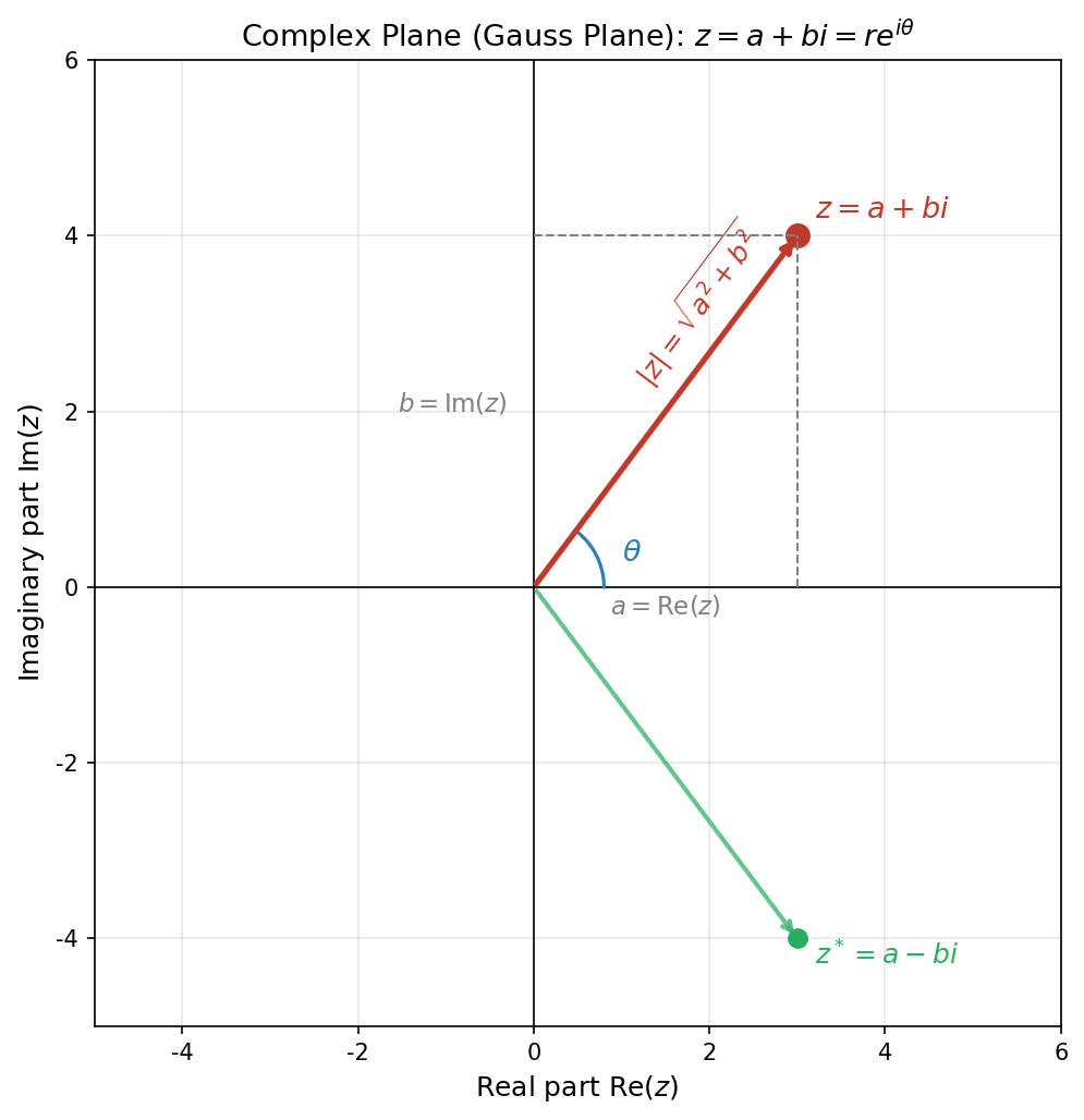
Fig. 4.1: Representation of the complex number \(z = a + bi\) on the complex plane. The absolute value \(|z| = \sqrt{a^2+b^2}\) is the distance from the origin, and the argument \(\theta\) is the angle from the real axis. The complex conjugate \(z^* = a - bi\) is the reflection across the real axis.
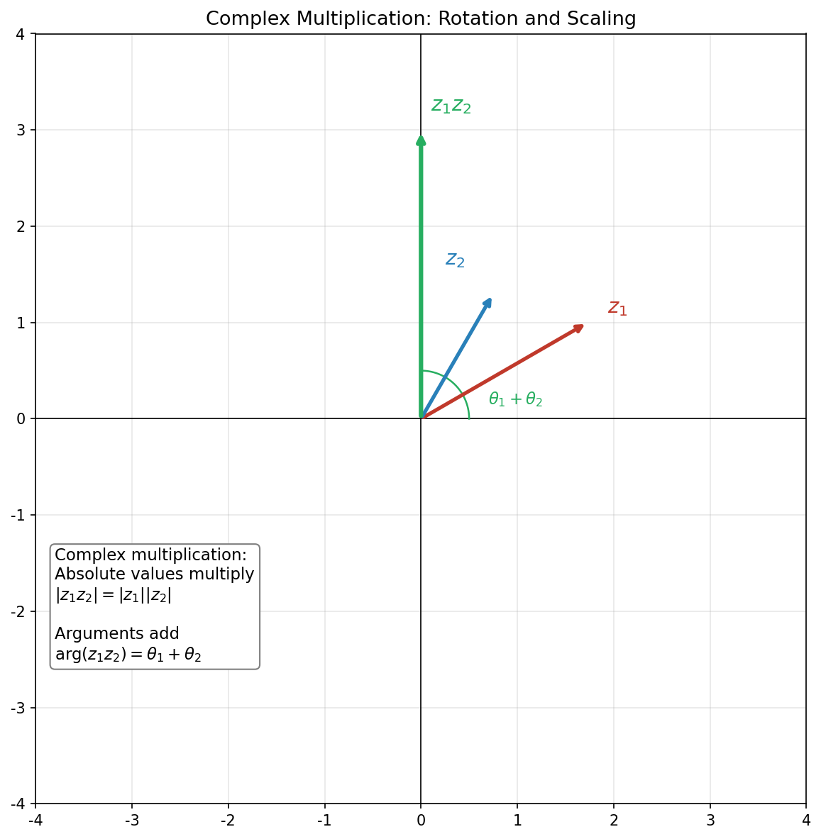
Fig. 4.2: Geometric meaning of complex number multiplication. The absolute value of \(z_1 z_2\) is \(|z_1|\cdot|z_2|\) (scaling), and the argument is \(\theta_1 + \theta_2\) (rotation). Multiplying by \(i\) corresponds to "rotation by \(90°\)."
✅ Comprehension Check: Find the absolute value \(|z|\) and the value of \(z \cdot z^*\) for the complex number \(z = 3 + 4i\).
Answer
\(|z| = \sqrt{3^2 + 4^2} = \sqrt{9 + 16} = \sqrt{25} = 5\). \(z \cdot z^* = (3 + 4i)(3 - 4i) = 9 + 16 = 25 = |z|^2\).
📝 Exercises:
- Polar form representation of complex numbers and geometric meaning of multiplication → Problem B-1. Absolute Value and Complex Conjugate of Complex Numbers
4.2 What Is a Probability Amplitude? — The First Rule
🟡 Lina: Now that we have our tools ready, let's dive into the heart of quantum mechanics. In the previous chapter, we saw that the results of the double-slit experiment cannot be explained by classical addition of probabilities (real numbers). Quantum mechanics introduces a quantity called the probability amplitude in place of probability.
🔵 Kai: "Amplitude"—is it like the amplitude of a wave?
🟡 Lina: The name originates from there, but it's a more general concept. Let me state the definition.
The First Rule (Law of Probability)
The probability \(P\) that an event occurs is given by the absolute value squared of the probability amplitude \(\phi\) (generally a complex number) corresponding to that event.
\[P = |\phi|^2 \tag{4.9}\]
🔵 Kai: Wait, that's it? But... why complex numbers? Probability is a real number between 0 and 1. What's the point of going through complex numbers?
🟡 Lina: That's a question that strikes at the heart of the matter. There are two reasons. First, since \(|z|^2 = a^2 + b^2 \geq 0\), the absolute value squared of a complex number is always a non-negative real number. Since probability must be non-negative, this condition is properly satisfied.
Of course, probability must also be at most 1, but this is guaranteed by appropriately normalizing the amplitudes. "Normalization" means the condition that the probabilities of all possible outcomes sum to exactly 1. For example, if there are 3 possible outcomes (\(A\), \(B\), \(C\)) with respective amplitudes \(\phi_A\), \(\phi_B\), \(\phi_C\), then \(|\phi_A|^2 + |\phi_B|^2 + |\phi_C|^2 = 1\) must hold. In classical probability too, there's the condition "the sum of probabilities of all cases equals 1." It's the same idea. The specific method will be covered in detail from Ch. 5 onward.
Note that in this chapter, since the goal is to see the effects of interference, I'll sometimes use amplitude values directly without worrying about normalization. As a result, computed values may exceed 1, but this is fine since they're pre-normalization values. For example, later we'll get values like \(|\phi_1|^2 + |\phi_2|^2 = 2\), but think of this as "a quantity proportional to probability" rather than "the probability itself." To get the true probability, you'd divide by the total to make it sum to 1—for instance, if the total is 2, divide each term by 2—but right now, only the relative change of "whether the value increases or decreases due to the interference term" matters, so I'll omit the division. The formal method of normalization will be learned in Ch. 5.
🔵 Kai: I see, normalization is deferred, and for now we just focus on whether interference increases or decreases things. But why bother with complex numbers?
🟡 Lina: The second reason—and this is the essential one—complex numbers have phase (argument \(\theta\)). When you add two complex numbers, depending on the phase difference, they can constructively or destructively interfere. This is the true nature of interference. Classical probabilities are always positive real numbers, so adding probabilities always increases the total—weakening can never occur, right?
⚪ Mei: I see. Probabilities are always positive, so adding them always increases the total. But amplitudes are complex numbers, so when added, they can cancel each other out. That's what creates the "dark parts" of the interference pattern.
🟡 Lina: Exactly. This is the heart of quantum mechanics. Instead of adding probabilities directly, we add amplitudes and then take the absolute value squared. This difference in order creates the decisive distinction between classical and quantum.
🔵 Kai: But if amplitudes are complex numbers, that means they can't be directly measured in experiments, right? Measured values are always real numbers...
🟡 Lina: Sharp observation. That's correct. What we can directly observe in experiments is only \(|\phi|^2\), that is, probability. The amplitude itself cannot be directly measured. However, predictions from models using amplitudes match experimental results with astonishing accuracy. "Amplitudes cannot be directly seen, but without amplitudes we cannot explain experiments"—this is the power of quantum mechanics as a model.
🔵 Kai: Can't be seen, but can't do without...
🟡 Lina: Right. As we discussed in the prologue, the value of a physics model lies in "quantitative predictions and falsifiability," not in "truth." The probability amplitude model is the best hypothesis that, so far, has no contradictions with experiments.
Introducing Notation — Dirac's Bra-Ket
🟡 Lina: Let me introduce a convenient notation for writing probability amplitudes. It's the bra-ket notation invented by Dirac, widely used in quantum mechanics.
🟡 Lina: "The amplitude for a particle starting in state \(s\) and arriving at state \(x\)" is written as
The \(| s \rangle\) on the right is called a ket, and the \(\langle x |\) on the left is called a bra. In this notation, the ket represents the initial state and the bra represents the final state. The whole \(\langle x | s \rangle\) is called a bracket (= bra + ket), and it's the symbol meaning "the amplitude from \(s\) to \(x\)." Bras and kets have deeper mathematical meaning, but that will be covered in Ch. 11. For now, use them as "shorthand symbols for writing amplitudes."
🔵 Kai: Why is the final state on the left? Does that mean you read from right to left in time order?
🟡 Lina: Yes, read from right to left as "starting from \(s\), arriving at \(x\)." It takes some getting used to at first, but when matrix calculations appear in later chapters, this "right to left" convention connects naturally. We'll start using it right away from the next Ch. 5, but let's get familiar with the notation by actually computing there.
🟡 Lina: Using this notation, the first rule can be written as
⚪ Mei: Since the amplitude symbol itself expresses "from where to where," the probability formula becomes easier to read too.
✅ Comprehension Check: In Dirac's bra-ket notation \(\langle x | s \rangle\), what do the ket \(|s\rangle\) and bra \(\langle x|\) represent respectively? Also, what does this entire symbol physically mean?
Answer
The ket \(|s\rangle\) represents the initial state, and the bra \(\langle x|\) represents the final state. The entire symbol \(\langle x | s \rangle\) means "the probability amplitude for a particle starting in state \(s\) and arriving at state \(x\)." It is read from right to left.
✅ Comprehension Check: State in one sentence why it is essentially important that probability amplitudes are complex numbers rather than real numbers.
Answer
Because complex numbers have phase (argument), constructive reinforcement or cancellation (interference) can occur when two amplitudes are added, whereas with only positive real numbers, cancellation cannot occur.
4.3 Adding Paths — The Second Rule
🟡 Lina: Next, let's move on to the second rule. This is the rule that directly answers the "mystery" we saw in Ch. 3.
The Second Rule (Addition Law for Amplitudes)
When an event can be realized through multiple indistinguishable paths, the total amplitude is the sum of the amplitudes for each path.
🔵 Kai: What does "indistinguishable paths" mean?
🟡 Lina: It means "there is no way, in principle, to know which path the particle took." In the double-slit experiment, when you don't observe which slit it went through, the path through slit 1 and the path through slit 2 are "indistinguishable."
In the double-slit case, the amplitude at detector position \(x\) is
🟡 Lina: Now recall the discussion from the previous chapter. Classically, we added probabilities directly as \(P = P_1 + P_2\). But in quantum mechanics, we add amplitudes and then compute the probability. That is,
Here I've abbreviated \(\phi_1 = \langle x | s \rangle_{\text{via slit 1}}\), \(\phi_2 = \langle x | s \rangle_{\text{via slit 2}}\).
⚪ Mei: The left side is the quantum mechanical prediction, and the right side is the classical prediction. These two are generally not equal.
🔵 Kai: But what does that "difference" look like concretely? When you add complex numbers and then take the absolute value, it's not a simple subtraction, right?
🟡 Lina: Good question. Let's actually expand it. When \(\phi_1\) and \(\phi_2\) are complex numbers,
From the first line to the second, I used \((\phi_1 + \phi_2)^* = \phi_1^* + \phi_2^*\)—since taking the complex conjugate "flips the imaginary part of each term separately," the conjugate of a sum is the sum of conjugates. The third line is just expanding by the distributive law. And using equation (4.6)'s \(z \cdot z^* = |z|^2\), I rewrote \(\phi_1\phi_1^* = |\phi_1|^2\) and \(\phi_2\phi_2^* = |\phi_2|^2\).
🔵 Kai: Ah, the \(z \cdot z^* = |z|^2\) we just learned is already being used!
🟡 Lina: The last two terms \(\phi_1 \phi_2^* + \phi_1^* \phi_2\) are called the interference term. The essence of interference is packed in here.
🔵 Kai: Wait a moment. \(\phi_1 \phi_2^*\) is a complex number, right? The probability \(P\) must be a real number, so is it okay to have complex terms in there? Is there some relationship with the other term \(\phi_1^* \phi_2\)?
🟡 Lina: Good question, and good insight. That's exactly right—\(\phi_1 \phi_2^*\) and \(\phi_1^* \phi_2\) are complex conjugates of each other. When you add complex conjugates, the imaginary parts cancel and you get a real number—for example, \((a+bi) + (a-bi) = 2a\), right? So the interference term is always real, and the condition that \(P\) should be real is properly satisfied.
🔵 Kai: Oh, that's true. Adding \(w\) and \(w^*\) eliminates the imaginary part, so for any \(\phi_1\), \(\phi_2\), the interference term is real.
🟡 Lina: Moreover, this structure holds the same way even when there are three or more amplitudes. If you expand \(|\phi_1 + \phi_2 + \cdots|^2\), all cross terms appear as pairs \(\phi_j\phi_k^*\) and \(\phi_j^*\phi_k\), so the probability being real is automatically guaranteed regardless of the number of amplitudes.
⚪ Mei: So the structure of "appearing in complex conjugate pairs guarantees a real result" works automatically no matter how many amplitudes there are.
🟡 Lina: Right. To make it more visible, let's write each amplitude in polar form. As we saw in equation (4.7), \(\phi_1 = |\phi_1|(\cos\theta_1 + i\sin\theta_1)\), \(\phi_2 = |\phi_2|(\cos\theta_2 + i\sin\theta_2)\). Let me introduce just one convenient shorthand. We write \(e^{i\theta} = \cos\theta + i\sin\theta\). This is called Euler's formula.
🔵 Kai: Wait a moment. \(e\) is the base of the exponential function, \(2.718\ldots\), right? What does it mean to put the imaginary number \(i\theta\) in the exponent?
🟡 Lina: Good question. A perfectly reasonable doubt. In the real number domain, \(e^x\) is just "\(e\) multiplied \(x\) times," but when the exponent is imaginary, that interpretation doesn't directly work. Euler's formula emerges naturally when you rewrite the exponential function as an infinite sum (infinite series). That derivation is done carefully in Appendix A. At this stage, define it as follows—\(e^{i\theta}\) means \(\cos\theta + i\sin\theta\). That is, we're giving the name \(e^{i\theta}\) to "the complex number with absolute value 1 and argument \(\theta\)." Think of it not so much as a shorthand but as a definition of a new symbol. The greatest advantage of this definition is that multiplication becomes addition of exponents—\(e^{i\alpha} \cdot e^{i\beta} = e^{i(\alpha+\beta)}\). This is just expressing in exponential notation the property we demonstrated in equation (4.8) that "when you multiply two complex numbers, the arguments add." So it's not a new law but a rewriting of an already confirmed fact.
Let's verify concretely. In equation (4.8) we had \(r_1(\cos\theta_1 + i\sin\theta_1) \cdot r_2(\cos\theta_2 + i\sin\theta_2) = r_1 r_2[\cos(\theta_1+\theta_2) + i\sin(\theta_1+\theta_2)]\). Rewriting this with \(e^{i\theta}\) gives \(r_1 e^{i\theta_1} \cdot r_2 e^{i\theta_2} = r_1 r_2 \, e^{i(\theta_1+\theta_2)}\)—the exact same content, written much more compactly.
🔵 Kai: I see, it's just a different way of writing equation (4.8). Multiplication becomes addition, so it's convenient. I'll use it as a shorthand for now.
🟡 Lina: Right. Using this notation, we can write \(\phi_1 = |\phi_1|e^{i\theta_1}\), \(\phi_2 = |\phi_2|e^{i\theta_2}\). Let me verify what happens when we take the complex conjugate. The complex conjugate of \(e^{i\theta} = \cos\theta + i\sin\theta\) just flips the sign of the imaginary part, giving \(\cos\theta - i\sin\theta\).
🔵 Kai: I understand that. But can \(\cos\theta - i\sin\theta\) be rewritten in the \(e\) form?
🟡 Lina: Good question. Recall the properties of trigonometric functions you learned in high school—\(\cos(-\theta) = \cos\theta\), \(\sin(-\theta) = -\sin\theta\). This follows directly from the unit circle definition. On the unit circle, the point at angle \(\theta\) is \((\cos\theta,\, \sin\theta)\), and the point at angle \(-\theta\) is symmetric about the real axis (\(x\)-axis), so the \(x\)-coordinate (\(\cos\)) is the same and the \(y\)-coordinate (\(\sin\)) has opposite sign. Therefore \(\cos\theta - i\sin\theta = \cos(-\theta) + i\sin(-\theta)\). Now recall our shorthand convention—\(e^{i\alpha} = \cos\alpha + i\sin\alpha\). Substituting \(\alpha = -\theta\), the right side is exactly \(e^{i(-\theta)} = e^{-i\theta}\). In other words, taking the complex conjugate flips the sign of the exponent.
⚪ Mei: I see, \((e^{i\theta})^* = e^{-i\theta}\). Simple.
🟡 Lina: So \(\phi_2^* = |\phi_2|e^{-i\theta_2}\). Then
where \(\delta = \theta_1 - \theta_2\) is the phase difference between the two amplitudes. Similarly, \(\phi_1^* \phi_2 = |\phi_1||\phi_2| e^{-i\delta}\). Let's expand using Euler's formula. \(e^{i\delta} = \cos\delta + i\sin\delta\), \(e^{-i\delta} = \cos\delta - i\sin\delta\). Adding these two, the imaginary parts cancel giving \(e^{i\delta} + e^{-i\delta} = 2\cos\delta\), so
🔵 Kai: Oh! It's \(\cos\delta\)! Depending on the value of \(\delta\), it can be positive or negative, so the interference term can be either positive or negative!
🟡 Lina: Right. To summarize:
- When \(\cos\delta = +1\) (phase difference \(\delta = 0\)): \(P = (|\phi_1| + |\phi_2|)^2\) → constructive interference (bright fringe)
- When \(\cos\delta = -1\) (phase difference \(\delta = \pi\)): \(P = (|\phi_1| - |\phi_2|)^2\) → destructive interference (dark fringe)
- If \(|\phi_1| = |\phi_2|\) and \(\delta = \pi\), then \(P = 0\) → complete cancellation
⚪ Mei: With just a phase difference, the probability can go all the way to zero. That's something that could never happen classically.
Look at Fig. 4.3 "Addition of probability amplitudes (on the complex plane)". When adding amplitudes as arrows (vectors) on the complex plane, you can see at a glance that when pointing in the same direction (same phase) the lengths add, and when pointing in opposite directions (opposite phase) they cancel.
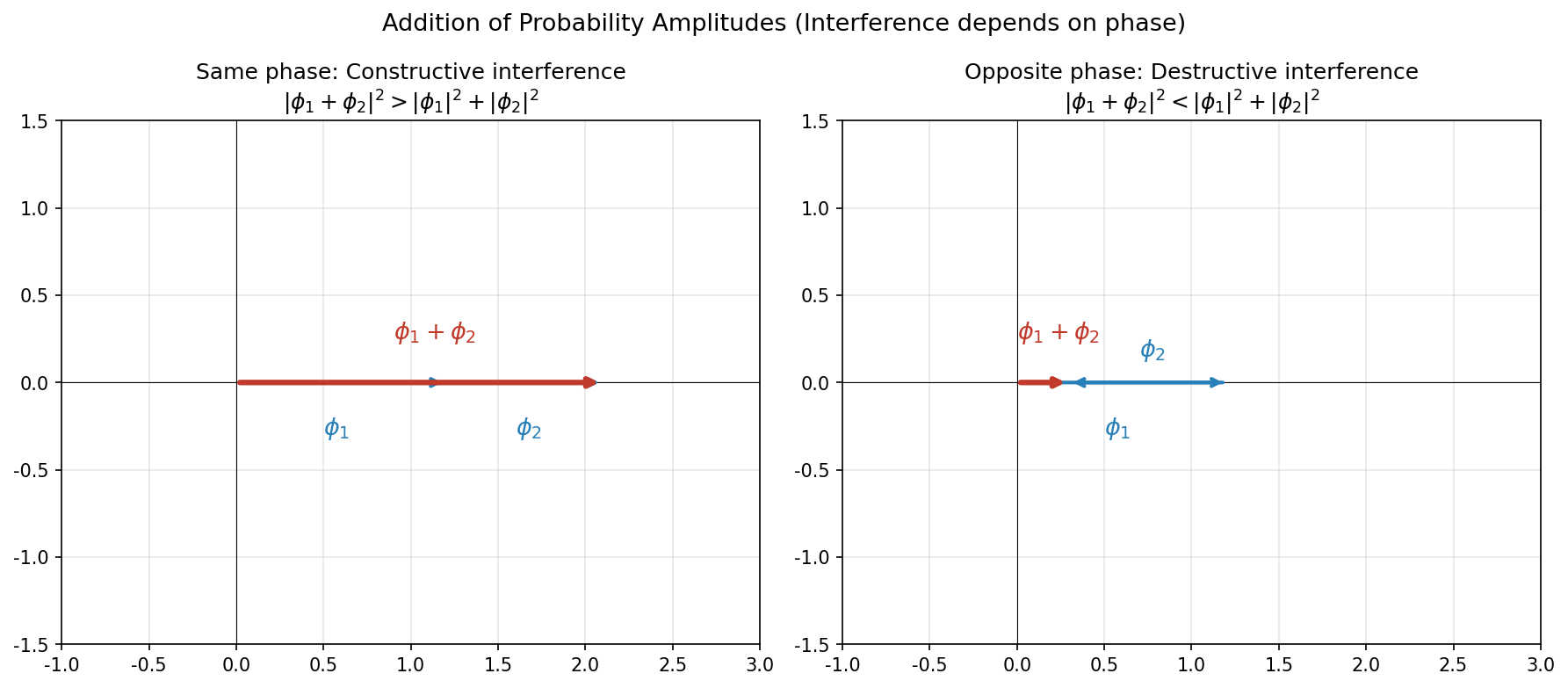
Fig. 4.3: Addition of probability amplitudes (on the complex plane). Left: In-phase case (\(\delta = 0\)), amplitudes constructively interfere giving \(|\phi_1 + \phi_2|^2 > |\phi_1|^2 + |\phi_2|^2\). Right: Anti-phase case (\(\delta = \pi\)), amplitudes destructively interfere giving \(|\phi_1 + \phi_2|^2 < |\phi_1|^2 + |\phi_2|^2\). The phase difference is the true nature of interference.
🔵 Kai: So this is the true nature of interference fringes...! Because amplitudes are complex numbers, phase differences arise, and when added they can reinforce or cancel. If you added probabilities directly, this wouldn't happen.
🟡 Lina: Right. And look at the third term \(2|\phi_1||\phi_2|\cos\delta\) in equation (4.14)—this is precisely what corresponds to the interference term observed as the "deviation from the classical prediction \(P_1 + P_2\)" in Ch. 3. With just the first and second rules, we've reproduced that experimental fact as a formula.
⚪ Mei: So the "deviation" we saw experimentally in the previous chapter—its true identity was this \(\cos\delta\) term.
Generalization: Many Paths
🟡 Lina: The second rule is not limited to two paths. If there are \(N\) indistinguishable paths,
For example, if the wall has 5 slits, you add all 5 amplitudes. If there are multiple walls, each with multiple slits, you add the amplitudes for all possible paths.
🔵 Kai: What if there are infinitely many paths?
🟡 Lina: Sharp question. In fact, Feynman went exactly in that direction and arrived at the path integral formulation, which "sums the amplitudes of all possible paths." That's a topic for later, but remember that it's a natural extension of the second rule.
✅ Comprehension Check: In the interference term \(2|\phi_1||\phi_2|\cos\delta\), what is the value of the interference term when \(\delta = \pi/2\)? What physical situation does this correspond to?
Answer
Since \(\cos(\pi/2) = 0\), the interference term is 0. In this case, the probability becomes \(|\phi_1|^2 + |\phi_2|^2\), giving the same result as classical addition of probabilities. It is an intermediate situation where neither constructive nor destructive interference occurs.
✅ Comprehension Check: When two amplitudes \(\phi_1 = 1\), \(\phi_2 = e^{i\pi} = -1\) are added, what is the probability \(P = |\phi_1 + \phi_2|^2\)? Also, what is \(P_{\text{cl}} = |\phi_1|^2 + |\phi_2|^2\) when probabilities are added classically?
Answer
\(\phi_1 + \phi_2 = 1 + (-1) = 0\) so \(P = |0|^2 = 0\) (complete cancellation). On the other hand, \(P_{\text{cl}} = |1|^2 + |-1|^2 = 1 + 1 = 2\). In quantum mechanics, the probability can be zero, but classical addition never gives zero. (Note: \(P_{\text{cl}} = 2 > 1\) is a pre-normalization value so there's no problem. What matters in this example is the qualitative difference that "in quantum mechanics \(P = 0\) is possible.")
📝 Exercises:
- Number of interference terms for the case of 3 slits → Problem M-2. Interference Pattern from \(N\) Equally-Spaced, Equal-Amplitude Slits
4.4 Multiplying Processes — The Third Rule
🟡 Lina: Let's move on to the third rule.
The Third Rule (Multiplication Law for Amplitudes)
When a particle travels along a certain path, the amplitude for the entire path is the product of the amplitudes for each stage that constitutes the path.
🔵 Kai: Multiplication, not addition? When do you multiply?
🟡 Lina: You "add" for parallel alternatives (which path to take), and you "multiply" for sequential stages (things that happen in order within a single path). Why multiplication? Because even in classical probability, the probability of "A happens, and then B also happens" is \(P(A) \times P(B)\) (for independent events). The same idea applies to amplitudes—the amplitude for a single path where "the first stage occurs, then the second stage occurs" is the product of the amplitudes for each stage.
For example, if the path "from Tokyo to Osaka" consists of two stages "Tokyo → Nagoya" and "Nagoya → Osaka," the amplitude for the entire path is the product of the amplitudes for each stage. In the double-slit experiment, the amplitude for "the path through slit 1" is
Reading from right to left, it's the product of "the amplitude to reach slit 1 from \(s\), \(\langle 1 | s \rangle\)" and "the amplitude to reach \(x\) from slit 1, \(\langle x | 1 \rangle\)."
⚪ Mei: Same structure as classical probability multiplication. But...
🔵 Kai: But amplitudes are complex numbers, right? Does multiplying complex numbers produce something different from multiplying real probabilities?
🟡 Lina: Good question. There's a decisive difference. Multiplying probabilities is "positive real × positive real = positive real," so phase doesn't come into play. Multiplying amplitudes is "complex number × complex number = complex number," and phases add up. As we saw in equation (4.8), arguments are summed, right? This accumulation of phase determines the interference pattern when amplitudes are later added together.
🔵 Kai: I see. Phases accumulate through multiplication, and then interference occurs due to those phase differences when you add. Multiplication and addition work as a set.
✅ Comprehension Check: What is the decisive difference between classical probability multiplication and quantum mechanical amplitude multiplication?
Answer
Classical probability multiplication is the product of positive real numbers, so there's no concept of phase. Quantum mechanical amplitude multiplication is the product of complex numbers, so phases (arguments) are added. This accumulation of phase determines the interference pattern when amplitudes are subsequently added together.
Summary of the Three Rules
🟡 Lina: Let me summarize the three rules here.
Table 4.1: The three fundamental rules of quantum mechanics
| Rule | Content | Formula |
|---|---|---|
| First Rule | Probability = absolute value squared of amplitude | $P = |
| Second Rule | Indistinguishable paths → add amplitudes | \(\phi = \phi_1 + \phi_2 + \cdots\) |
| Third Rule | Successive processes → multiply amplitudes | \(\phi = \phi_A \cdot \phi_B \cdot \cdots\) |
🔵 Kai: Only three? That's all of quantum mechanics?
🟡 Lina: Saying "all" is an overstatement, but a surprisingly large number of phenomena are derived from these three rules. Look at Fig. 4.4 "Structure of the three rules. Left: Second rule". The second rule (addition) corresponds to parallel alternatives, and the third rule (multiplication) corresponds to sequential stages.
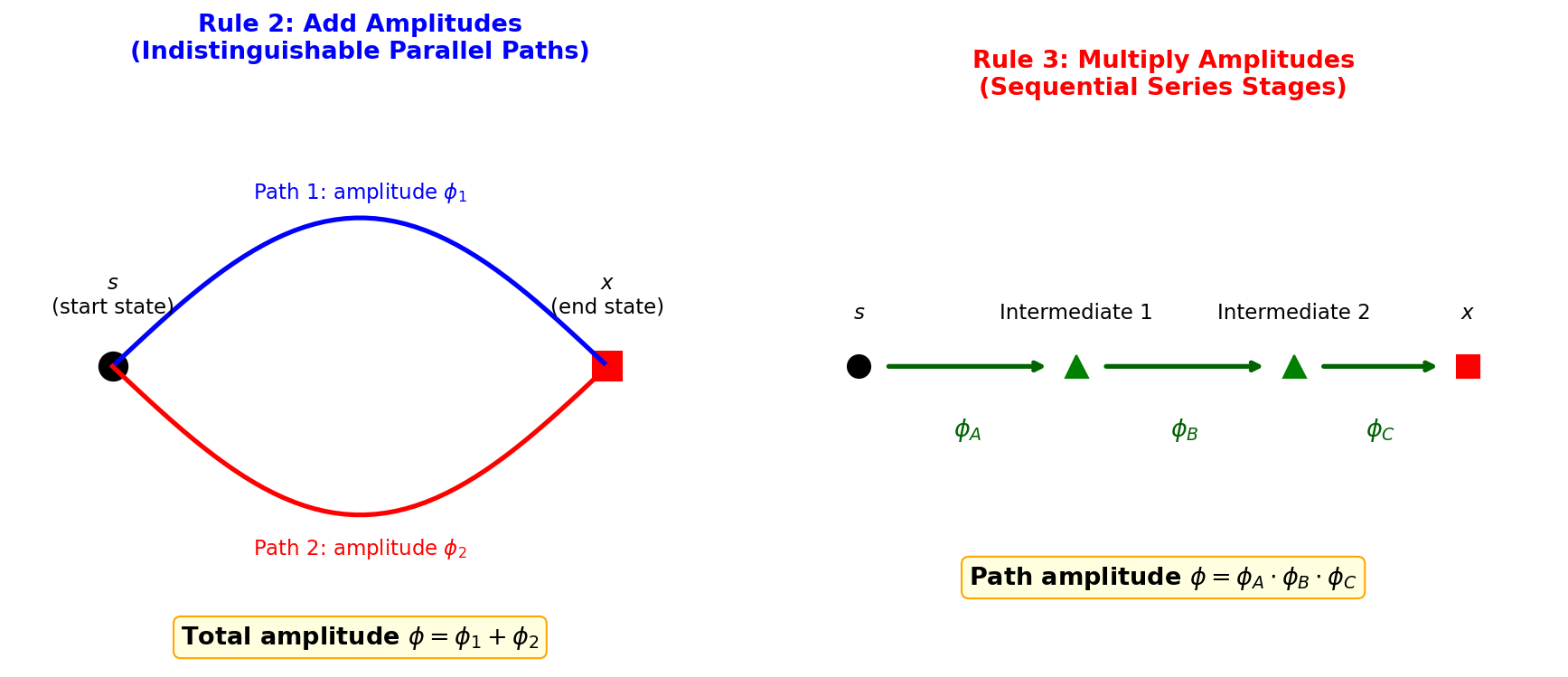
Fig. 4.4: Structure of the three rules. Left: Second rule—add amplitudes for indistinguishable parallel paths from initial state \(s\) to final state \(x\) (\(\phi = \phi_1 + \phi_2\)). Right: Third rule—multiply amplitudes for successive serial stages constituting a single path (\(\phi = \phi_A \cdot \phi_B \cdot \phi_C\)).
🟡 Lina: Feynman presented these three rules as the starting point of quantum mechanics. Of course, to solve specific problems, you need to separately know "what values each stage's amplitude takes." But the structure of the rules is complete with these three. It's similar to how in classical mechanics, Newton's equation of motion \(\mathbf{F} = m\mathbf{a}\) provides the "structure," while the specific form of the force \(\mathbf{F}\) differs from problem to problem.
⚪ Mei: So the three rules determine the framework of "how to calculate," and the specific amplitude values are given separately for each system.
✅ Comprehension Check: In what situations do you use the second rule (addition) and the third rule (multiplication), respectively?
Answer
Second rule (addition): When a particle has multiple indistinguishable paths from the same initial state to the same final state, add the amplitudes for each path. Third rule (multiplication): When a single path is composed of multiple successive stages, multiply the amplitudes for each stage.
📝 Exercises:
- Calculating amplitudes for the case of passing through 2 walls → Problem M-4. Calculating Amplitudes Through Two Walls
4.5 Re-describing the Double Slit with Amplitudes — Integration of the Three Rules
🟡 Lina: Now let's use all three rules to quantitatively describe the double-slit experiment from Ch. 3 using amplitudes. This is today's climax.
Confirming the Setup
🟡 Lina: Let me confirm the experimental arrangement (recall the figure from Ch. 3).
- Electron source \(s\)
- A wall with slit 1 and slit 2
- A detector at position \(x\) on the other side of the wall
Which slit the electron passes through is not observed.
🟡 Lina: I've summarized the experimental arrangement and amplitude labels in Fig. 4.5 "Structure of amplitudes in the double-slit experiment". Let's apply the three rules in order while looking at this figure.
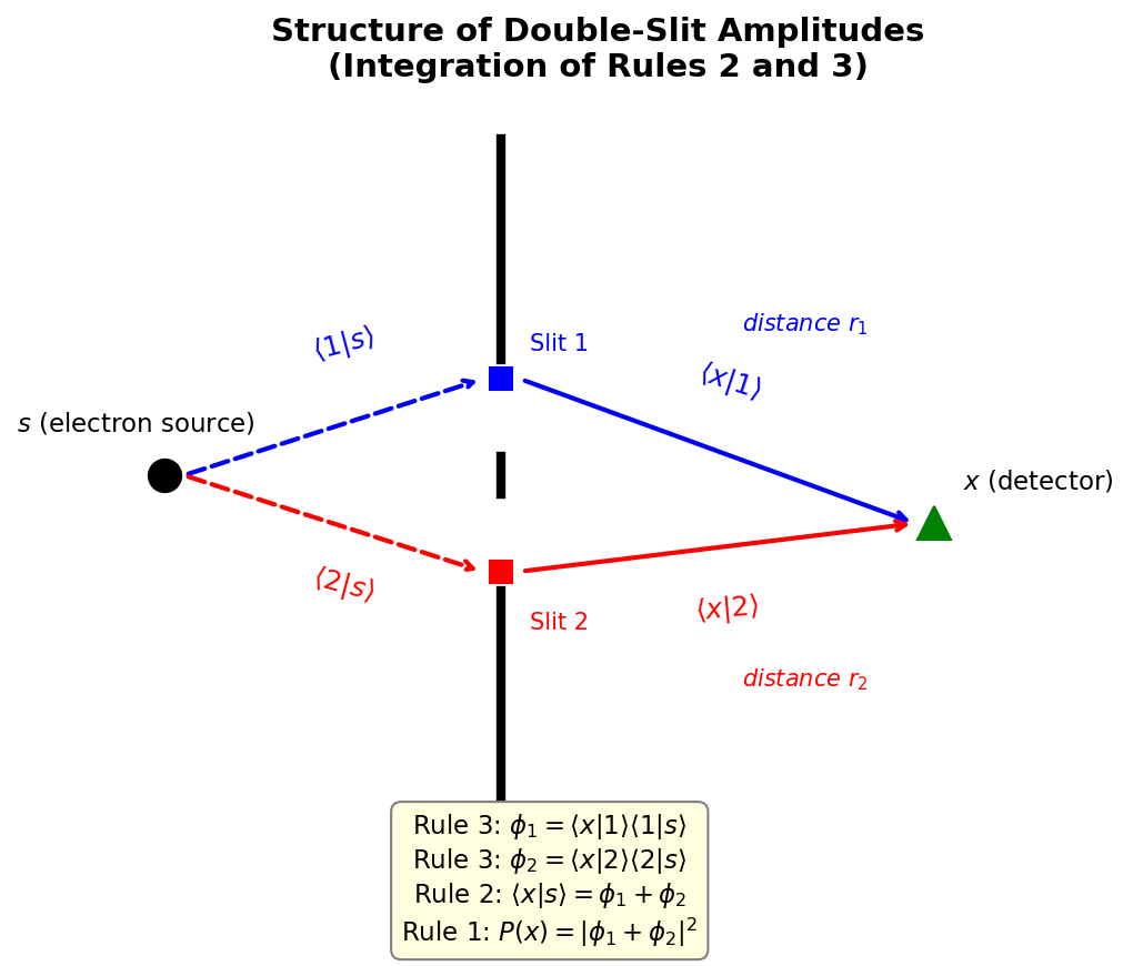
Fig. 4.5: Structure of amplitudes in the double-slit experiment. Two paths from electron source \(s\) via slits 1, 2 to detector \(x\). By the third rule, each path's amplitude is the product of stages (e.g., \(\phi_1 = \langle x|1\rangle\langle 1|s\rangle\)); by the second rule, the total amplitude is \(\phi_1 + \phi_2\); by the first rule, the probability is \(|\phi_1 + \phi_2|^2\).
Step 1: Writing Each Path's Amplitude Using the Third Rule
🟡 Lina: First, let's write each path's amplitude using the third rule (multiplication).
Amplitude for the path via slit 1:
Amplitude for the path via slit 2:
🔵 Kai: Reading from right to left, it's "\(s\) to the slit" × "slit to \(x\)."
Step 2: Finding the Total Amplitude Using the Second Rule
🟡 Lina: Since we don't observe which slit the electron passes through, the two paths are indistinguishable. By the second rule (addition):
Step 3: Finding the Probability Using the First Rule
🟡 Lina: Finally, by the first rule (probability = |amplitude|²):
This is the same form as equation (4.12). The last two terms equal \(2|\phi_1||\phi_2|\cos\delta\) from equation (4.13) (where \(\delta\) is the phase difference between \(\phi_1\) and \(\phi_2\)—we'll see what specifically determines it right after this). By the way, since \(w + w^* = 2\,\mathrm{Re}(w)\) (twice the real part) holds for any complex number \(w\), the interference term can also be written as \(2\,\mathrm{Re}(\phi_1 \phi_2^*)\).
⚪ Mei: Just by applying the three rules in order, the interference term we derived earlier appears directly.
The Physical Origin of the Phase Difference
🔵 Kai: But how is \(\delta\) specifically determined?
🟡 Lina: Good question. Recall the de Broglie relation we learned in Ch. 2. A particle with momentum \(p\) has a corresponding wavelength \(\lambda = h/p\).
🔵 Kai: I remember the wavelength. But what does "phase advances" specifically mean?
🟡 Lina: Good question. Let me explain "phase" intuitively first. When we represent a wave as \(\cos\theta\), the value of \(\theta\) is the phase. \(\theta = 0\) is a crest, \(\theta = \pi\) is a trough, and \(\theta = 2\pi\) returns to a crest. In other words, phase is the angle representing "which stage of the wave's cycle we're at." In complex number terms, the argument \(\theta\) of \(e^{i\theta}\) corresponds exactly to this phase.
🔵 Kai: I see, as the phase goes \(0 \to \pi \to 2\pi\), the wave goes crest → trough → crest through one full cycle.
🟡 Lina: Right. To be more specific, recall the wave equation from high school—for a wave with wavelength \(\lambda\), if \(r\) is the distance from the starting point along the direction of propagation, the wave value is represented as \(\cos\bigl(\frac{2\pi}{\lambda}r\bigr)\). The \(\frac{2\pi}{\lambda}r\) part is the phase. At \(r = 0\) the phase is \(0\) (crest), at \(r = \lambda/2\) the phase is \(\pi\) (trough), at \(r = \lambda\) the phase is \(2\pi\) (crest again). In other words, the wavelength \(\lambda\) is "the distance over which the wave repeats one full period (crest → trough → crest)," and when it travels a distance \(\lambda\), the phase advances by exactly \(2\pi\) (one full cycle).
🔵 Kai: I see, one wavelength corresponds to \(2\pi\) of phase advance. So three wavelengths would be \(6\pi\)?
🟡 Lina: Exactly. Let me generalize this. When a particle moves a distance \(r\), the wave completes \(r/\lambda\) cycles within that distance. Therefore the phase advances by \(2\pi \times (r/\lambda) = 2\pi r/\lambda\). If \(r = 3\lambda\), then \(6\pi\)—that's three repetitions of crest → trough → crest. Here I used \(\cos\) to build intuition about phase, but since quantum mechanical amplitudes are complex numbers, we actually handle phase as the argument \(\theta\) of \(e^{i\theta}\). That is, when a particle moves a distance \(r\), the argument (= phase) of the amplitude rotates by \(2\pi r/\lambda\)—in the polar form we learned earlier, this means multiplying the amplitude by a complex number with absolute value 1 and argument \(2\pi r/\lambda\). The conclusion "when a particle moves a distance \(r\), the phase advances by \(2\pi r/\lambda\)" is the same regardless of which notation we use.
⚪ Mei: So the content we grasped intuitively with \(\cos\) translates directly to the story of the argument of \(e^{i\theta}\).
🔵 Kai: I understand phase advancing, but how does it affect the amplitude?
🟡 Lina: Recall the polar form we just learned. The amplitude can be written as \(|\phi|e^{i\theta}\), where \(\theta\) is the phase. Since the phase increases by \(2\pi r/\lambda\) when a particle moves a distance \(r\), the argument of the amplitude also rotates by that amount. Written as a formula, the amplitude \(|\phi|e^{i\theta_0}\) at the starting point gets multiplied by the phase factor \(e^{i \cdot 2\pi r/\lambda}\):
This is exactly the property from equation (4.8) that "multiplication adds the arguments." The absolute value (magnitude) doesn't change—only the phase (direction) changes.
🔵 Kai: Oh, the magnitude stays the same and only the arrow's direction rotates. That's exactly "rotation."
🟡 Lina: Let's rewrite this using the de Broglie relation \(\lambda = h/p\).
🟡 Lina: Let's tidy up this expression. Looking at the form \(\frac{2\pi p}{h} \cdot r\), the combination \(\frac{2\pi}{h}\) appears as a common factor multiplying \(p\) and \(r\). In fact, whenever we express phase in angles (radians), \(2\pi\) and \(h\) always appear as a set. In Ch. 1, when we wrote Bohr's quantization condition, we introduced the symbol \(\hbar = h/(2\pi)\), remember? Back then we used it for quantization of angular momentum, but the same symbol naturally appears here too. To confirm:
read as "h-bar."
🔵 Kai: I see, the \(\hbar\) that appeared in angular momentum quantization also shows up in phase calculations. But how does this change the equation?
🟡 Lina: Let's manipulate this definition. Multiplying both sides of \(\hbar = h/(2\pi)\) by \(2\pi\) gives \(2\pi\hbar = h\), that is, \(h = 2\pi\hbar\). So replacing \(h\) in \(2\pi p/h\) with \(2\pi\hbar\):
The \(2\pi\) cancels out cleanly, right? Using this, the phase expression from earlier becomes
nicely compact. In other words, the phase takes the form "momentum × distance" divided by \(\hbar\)—\(pr/\hbar\).
⚪ Mei: The phase is \(pr/\hbar\)—just momentum times distance divided by \(\hbar\). It settles into a simple form.
🟡 Lina: So when a free particle moves a distance \(r\), the phase advances by \(pr/\hbar\). Using the Euler notation we just learned, "phase advancing by \(\theta\)" corresponds to "multiplying the amplitude by \(e^{i\theta}\)." Therefore, the amplitude acquires a phase factor of
\(\hbar\) is "just \(h\) divided by \(2\pi\)," but when expressing phase in angles (radians), the \(2\pi\) gets absorbed and the formulas become cleaner, so in quantum mechanics \(\hbar\) is used more often than \(h\).
🔵 Kai: So the \(e^{i\theta}\) notation we introduced earlier gets used here. In other words, when a particle moves a distance \(r\), the magnitude of the amplitude doesn't change but the phase rotates by \(pr/\hbar\)?
🟡 Lina: Exactly. \(e^{ipr/\hbar}\) is a complex number with absolute value 1 and argument \(pr/\hbar\), so multiplying it by the amplitude doesn't change the magnitude—it only rotates the phase. "When a particle moves a distance \(r\), the phase rotates by \(pr/\hbar\)"—this is the fundamental behavior of a free particle's amplitude. Look at Fig. 4.6 "Phase accumulation of a free particle".
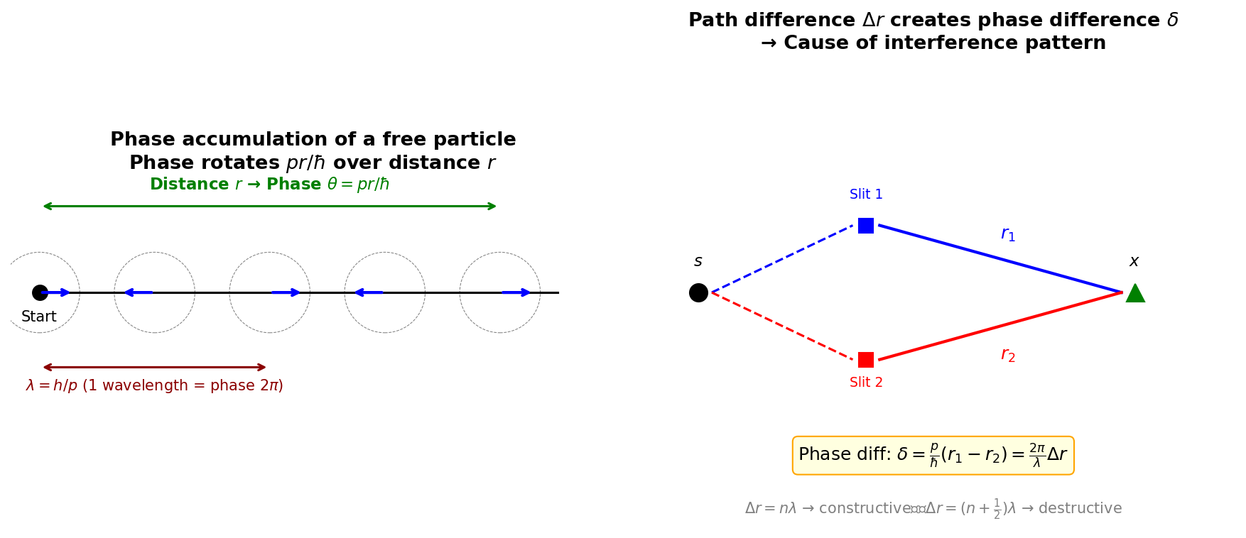
Fig. 4.6: Phase accumulation of a free particle. Left: When a particle moves a distance \(r\), the amplitude's phase rotates by \(pr/\hbar\) (the arrow direction represents phase). After traveling one wavelength \(\lambda = h/p\), the phase rotates by \(2\pi\). Right: In the double slit, when the two paths have different lengths, a phase difference \(\delta = p\Delta r/\hbar\) arises, which determines the interference pattern.
🟡 Lina: Let \(r_1\) be the distance from slit 1 to detector \(x\), and \(r_2\) the distance from slit 2 to \(x\). To simplify things, let's consider a symmetric arrangement where the electron source is centered directly in front of the two slits. When we multiply the amplitudes along each path by the third rule, since phases add in multiplication as we saw in equation (4.8), the total phase for path \(k\) is "phase from source to slit \(k\)" + "phase from slit \(k\) to \(x\)." In formulas, letting \(d_k\) be the distance from the source to slit \(k\) and \(r_k\) the distance from slit \(k\) to the detector, the total phase for path \(k\) is \(pd_k/\hbar + pr_k/\hbar\). The phase difference between the two paths is
In the symmetric arrangement, \(d_1 = d_2\), so the first term vanishes and the phase difference is determined only by the slit-to-detector part.
🔵 Kai: What if the electron source is off-center—would the conclusion change?
🟡 Lina: The conclusion doesn't change. In an asymmetric arrangement, "source → slit 1" and "source → slit 2" have different distances, so an extra phase difference is added. But this is a constant independent of the detector position \(x\), so it only shifts the entire interference pattern sideways—the fringe spacing and the fact that "interference occurs" remain the same. Since we want to see the mechanism of interference, let's use the symmetric arrangement which eliminates the extra constant.
Let me write the path difference as \(\Delta r = r_1 - r_2\). As we just learned, when a free particle moves a distance \(r\), the phase advances by \(pr/\hbar\). So the phase from slit \(k\) to detector \(x\) is \(\theta_k = pr_k/\hbar\). The phase difference \(\delta = \theta_1 - \theta_2\) is
⚪ Mei: The phase difference is proportional to the path difference \(\Delta r = r_1 - r_2\).
🟡 Lina: Right. And as you move the detector position \(x\), \(\Delta r\) changes, so \(\cos\delta\) oscillates and creates a bright-dark pattern—that's the interference fringes.
🔵 Kai: Just by shifting the detector position sideways, \(\cos\) oscillates... and that becomes the bright-dark pattern!
🟡 Lina: Let's transform this expression a bit more. First, from the definition \(\hbar = h/(2\pi)\), rewrite \(p/\hbar = 2\pi p/h\). Next, recall the de Broglie relation \(\lambda = h/p\) from Ch. 2. Solving for \(p\) gives \(p = h/\lambda\). Substituting:
In the middle step, I replaced \(p\) with \(h/\lambda\). The \(h\) cancels, and ultimately the phase difference is expressed using only the wavelength \(\lambda\) and the path difference \(\Delta r\).
Thus the phase difference is expressed using only the wavelength \(\lambda\) and the path difference \(\Delta r\).
When \(\Delta r\) is an integer multiple of the wavelength \(\lambda\) (\(\Delta r = \lambda, 2\lambda, 3\lambda, \ldots\)), \(\cos\delta = 1\) gives constructive interference; when it's a half-integer multiple (\(\Delta r = \lambda/2, 3\lambda/2, 5\lambda/2, \ldots\)), \(\cos\delta = -1\) gives destructive interference. This matches perfectly with the interference fringe pattern we observed experimentally in Ch. 3.
🔵 Kai: Amazing... Just with the three rules and the de Broglie relation, the double-slit interference pattern comes out quantitatively.
🟡 Lina: Yes. And nowhere in this derivation did we say "the electron is a wave." All we said was "probability amplitudes are complex numbers, and amplitudes for indistinguishable paths are added." Interference emerges naturally as a consequence of adding complex numbers.
✅ Comprehension Check: Is the assumption "electrons are waves" necessary to explain interference in the double-slit experiment? In the framework of the three rules, how is interference explained?
Answer
The assumption "electrons are waves" is not necessary. In the framework of the three rules, interference emerges naturally as a mathematical consequence of the rule that "probability amplitudes are complex numbers, and amplitudes for indistinguishable paths are added." Constructive and destructive interference due to phase differences creates the interference fringes.
✅ Comprehension Check: In the double-slit experiment, when the path difference \(\Delta r\) between the two paths is exactly equal to the de Broglie wavelength \(\lambda\), find the phase difference \(\delta\) and state the type of interference (constructive/destructive).
Answer
\(\delta = 2\pi\Delta r / \lambda = 2\pi\). Since \(\cos(2\pi) = 1\), this is constructive interference (bright fringe).
📝 Exercises:
- Derive the spacing of double-slit interference fringes from the amplitude formula → Problem M-3. Observation Destroys Interference: A Mathematical Explanation
4.6 Extension to More Complex Cases
🟡 Lina: To appreciate the power of the three rules, let's consider a slightly more complex case. There are 2 walls: the first has slits 1 and 2, and the second has 3 slits: \(a\), \(b\), \(c\).
🔵 Kai: The number of paths increases dramatically. \(s \to 1 \to a \to x\), \(s \to 1 \to b \to x\), ... how many total?
⚪ Mei: The first wall has 2 choices and the second has 3, so \(2 \times 3 = 6\) total.
🟡 Lina: I've illustrated all the paths in Fig. 4.7 "The case of 2 walls with multiple slits". The 6 lines of different colors represent all possible paths.
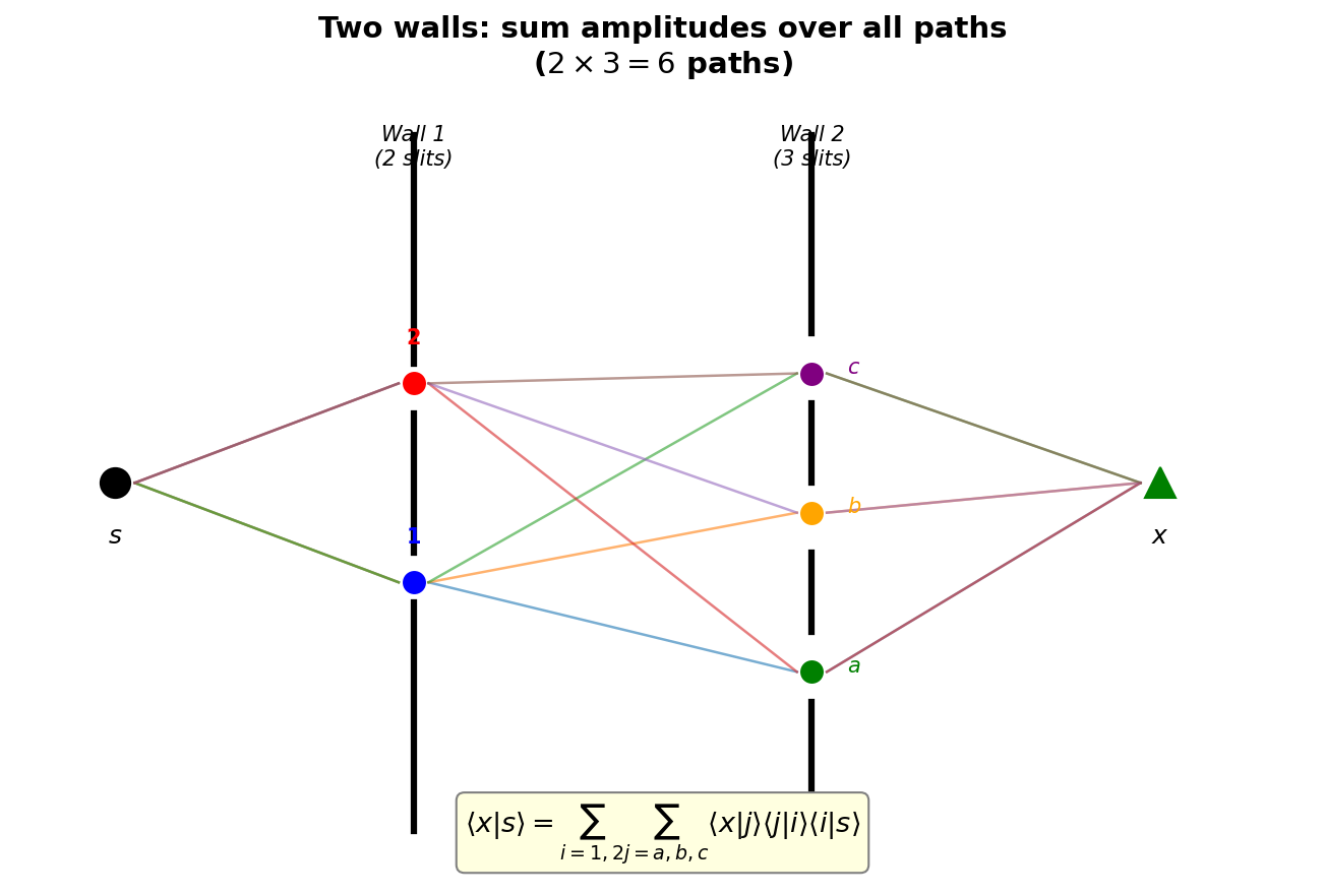
Fig. 4.7: The case of 2 walls with multiple slits. When wall 1 has 2 slits and wall 2 has 3 slits, there are \(2 \times 3 = 6\) paths from \(s\) to \(x\). Each path's amplitude is a product of 3 stages (third rule), and all path amplitudes are summed (second rule).
🟡 Lina: Write each path's amplitude using the third rule (multiplication), then add all paths using the second rule (addition).
🔵 Kai: There are 6 products of three amplitudes, and we add them all. The structure is the same as before.
🟡 Lina: Right. No matter how many walls or slits there are, the rules are the same. "Multiply each stage, add all paths." And finally, take the absolute value squared to get the probability.
⚪ Mei: Even as the number of walls and slits increases, the way the three rules are applied doesn't change.
🟡 Lina: Let me add an important point here. If you look closely at equation (4.24), the information about the first wall only appears in \(\langle j | i \rangle\) and \(\langle i | s \rangle\). The amplitude from the second wall onward, \(\langle x | j \rangle\), does not depend on which slit the particle passed through in the first wall.
🔵 Kai: So once the "state" after passing through the first wall is determined, you can forget the earlier details?
🟡 Lina: Exactly. Feynman put it this way—"All that is needed to predict the future is the amplitude at each slit." The details of where the particle came from before reaching a slit are all folded into the amplitude. This is the germ of the concept of "state" in quantum mechanics, which we'll treat in earnest from Ch. 5 onward.
✅ Comprehension Check: In the structure of equation (4.24), does the amplitude \(\langle x | j \rangle\) from the second wall's slit to the detector depend on which slit the particle passed through in the first wall? What physical meaning does this have?
Answer
It does not depend on it. The amplitude from slit \(j\) in the second wall to detector \(x\) is independent of which slit in the first wall the particle passed through to reach \(j\). This means "if you know the amplitude at a certain point, you can predict the future without knowing the details of the prior path," and represents the germ of the concept of "state" in quantum mechanics.
✅ Comprehension Check: If there are 3 walls with \(n_1\), \(n_2\), \(n_3\) slits in each wall respectively, how many total paths are there? Also, how many factors make up the product for each path's amplitude?
Answer
The total number of paths is \(n_1 \times n_2 \times n_3\). Each path's amplitude is a product of 4 factors (source → wall 1, wall 1 → wall 2, wall 2 → wall 3, wall 3 → detector).
📝 Exercises:
- Explicitly expand the total amplitude for the 2-wall case and count the number of interference terms → Problem M-1. Derivation of the General Formula for Interference Terms
4.7 The Boundary Between "Distinguishable" and "Indistinguishable"
🟡 Lina: Now, having seen the three rules and how to use them, let's discuss the most subtle and most important point in quantum mechanics. That is the boundary between "distinguishable" and "indistinguishable."
🔵 Kai: In Ch. 3, there was the discussion about "if you observe which slit it went through, the interference pattern disappears," right? Is this related?
🟡 Lina: Exactly. The three rules have an implicit premise.
Amplitudes are added only when the final states are indistinguishable.
When final states are distinguishable in principle, probabilities are added.
Destruction of Interference by Observation
🟡 Lina: Let's look at this concretely. Consider an experiment where we place a light source just behind each slit to detect which slit the electron passed through. Here's the setup—just behind the wall, at a position exactly midway between the two slits, we place one light source. And we place a photon detector \(D_1\) right next to slit 1, and a photon detector \(D_2\) right next to slit 2. So the arrangement from left to right is "\(D_1\) — slit 1 — light source — slit 2 — \(D_2\)." When a photon from the source hits the electron, it scatters—if the electron is near slit 1, the photon bounces toward slit 1's direction and enters \(D_1\); if it's near slit 2, it enters \(D_2\)—so which detector fires tells us the electron's position. This is a concrete apparatus realizing the "acquisition of path information" discussed in Ch. 3.
🔵 Kai: I see, you shine photons to find out "which one it's near." But then the interference disappears...
🟡 Lina: In this case, the amplitude for "the electron arrives at \(x\) AND the photon is detected at \(D_1\)" and the amplitude for "the electron arrives at \(x\) AND the photon is detected at \(D_2\)" correspond to different final states.
⚪ Mei: Not just "the electron is at \(x\)," but "where the photon is" is also part of the final state.
🟡 Lina: Right. The final state with the photon at \(D_1\) and the final state with the photon at \(D_2\) are distinguishable in principle. Therefore, we must not add the amplitudes. We add the probabilities.
🟡 Lina: Let's consider the case where the photon is detected at \(D_1\). Here we need to slightly broaden the application of the third rule.
The third rule states "multiply the amplitudes for each stage constituting a single path." Earlier we multiplied stages as a single particle moves "\(s\) → slit → \(x\)," but actually this rule is broader. It says to multiply the amplitudes of all events constituting a single scenario—even if multiple particles are involved.
🔵 Kai: Multiplication even when multiple particles are involved? Why is that?
🟡 Lina: Think of it this way—in classical probability too, the probability of "rolling a 1 on a die AND getting heads on a coin" is the product of each probability: \(1/6 \times 1/2\). The probability of independent events "occurring simultaneously" is multiplication. In quantum mechanics too, the third rule is exactly the amplitude version of this structure. "The electron passes through slit 1 and arrives at \(x\)" and "the photon scatters near slit 1 and goes to \(D_1\)" occurring simultaneously—these are multiple stages constituting a single scenario, so we directly apply the third rule (amplitudes for successive processes are multiplied) and get the product of each part's amplitude. The only difference from the classical case is that since they're complex numbers, phase is also multiplied in.
🔵 Kai: So "the electron does this" and "the photon does that" form one set, and the amplitude of the whole set is the product of each part? Same structure as probability multiplication, but with complex numbers so phase also comes in.
🟡 Lina: Exactly. The photon emitted from the light source is also a quantum, so its behavior is also described by amplitudes. Let \(a\) be the amplitude for a photon scattered near slit 1 to reach detector \(D_1\) when the electron passes through slit 1. The amplitude for the electron to pass through slit 1 and reach \(x\) is \(\phi_1\). The amplitude for this entire scenario is, by the third rule, \(a \cdot \phi_1 = a\phi_1\).
⚪ Mei: I see, the same structure Professor Lina just mentioned—"same structure as classical probability multiplication, but with complex numbers so phase is also multiplied in"—is being used here too.
🔵 Kai: Wait a moment. If a photon hits the electron, wouldn't it change the electron's motion? Can we still use \(\phi_1\) as is?
🟡 Lina: Good point. Strictly speaking, the interaction with the photon slightly changes the electron's momentum. But right now we want to see the essence of the argument—"distinguishability destroys interference"—so we're considering the case where the photon's influence is small (the electron's amplitude \(\phi_1\) barely changes). This approximation is good when the photon's energy is sufficiently small compared to the electron's kinetic energy. By the way, as we learned in Ch. 2, a photon's energy is \(E = hf\), so longer wavelength light has less energy and less influence on the electron. This point connects to later discussion.
🟡 Lina: Similarly, let \(b\) be the amplitude for the photon to scatter to \(D_1\) when the electron passed through slit 2. Since the number of symbols is growing, let me organize them here.
| Electron's path | Amplitude for photon going to \(D_1\) | Amplitude for photon going to \(D_2\) |
|---|---|---|
| Slit 1 | \(a\) (nearby) | \(b'\) (far side) |
| Slit 2 | \(b\) (far side) | \(a'\) (nearby) |
\(a\) and \(a'\) are amplitudes for "the photon goes to the detector near the slit the electron passed through," and \(b\) and \(b'\) are amplitudes for "going to the far detector." For a symmetric arrangement, \(a = a'\) and \(b = b'\).
🔵 Kai: I see, \(a\) is the amplitude for "going to the correct detector" and \(b\) is for "going to the wrong detector."
🟡 Lina: Right. Using these symbols, let's build the amplitudes for each final state.
🟡 Lina: First, consider the final state "electron is at \(x\) and photon is at \(D_1\)." There are 2 paths leading to this final state. One is via slit 1: multiply the amplitude \(\phi_1\) for the electron passing through slit 1 and reaching \(x\) by the amplitude \(a\) for the photon scattering near slit 1 and reaching \(D_1\), giving \(a\phi_1\) by the third rule. The other is via slit 2: similarly multiply \(\phi_2\) and \(b\) to get \(b\phi_2\). Both paths lead to the same final state (electron at \(x\), photon at \(D_1\)), so by the second rule we add the amplitudes:
🔵 Kai: Here too, "paths leading to the same final state → add amplitudes" applies directly.
🟡 Lina: Next, consider the final state "electron is at \(x\) and photon is at \(D_2\)." By the same logic, via slit 1 the photon goes to \(D_2\) with amplitude \(b'\) (far side), and via slit 2 with amplitude \(a'\) (nearby), so
🟡 Lina: Right. For a symmetric arrangement, \(a = a'\) and \(b = b'\). And if the light's wavelength is sufficiently shorter than the slit spacing, the photon can "distinguish" which slit the electron is near, so it goes almost certainly to the nearby detector—meaning \(b \approx 0\) and \(b' \approx 0\).
⚪ Mei: The shorter the wavelength, the stronger the "resolving power," so \(b\) approaches zero.
🟡 Lina: Now let's find the probability that the electron arrives at \(x\). The final states "photon at \(D_1\)" and "photon at \(D_2\)" are distinguishable in principle—you can tell by looking at the detector. For distinguishable final states, we add probabilities, not amplitudes. So
🔵 Kai: Wait, this is completely different from the \(|\phi_1 + \phi_2|^2\) in equation (4.20).
🟡 Lina: Right. If the light's wavelength is short enough that which slit was traversed can be perfectly determined (when \(b = 0\) and \(b' = 0\)), each term in equation (4.27) becomes \(|a\phi_1 + 0|^2 = |a\phi_1|^2\) and \(|0 + a'\phi_2|^2 = |a'\phi_2|^2\). Let me verify something about the absolute value of a product of two complex numbers. In equation (4.8), the absolute value of \(z_1 z_2\) was \(r_1 r_2 = |z_1|\cdot|z_2|\). That is, \(|z_1 z_2| = |z_1|\cdot|z_2|\)—the absolute value of a product is the product of absolute values. So \(|a\phi_1| = |a|\cdot|\phi_1|\), and its square is \(|a\phi_1|^2 = |a|^2|\phi_1|^2\). Therefore
Each term contains only \(\phi_1\) or only \(\phi_2\), and there are no terms mixing \(\phi_1\) and \(\phi_2\) (i.e., interference terms like \(\phi_1\phi_2^*\)). So the interference term vanishes. Here \(|a|^2\) and \(|a'|^2\) are photon scattering probabilities, which are generally not 1, but are constants independent of the detector position \(x\). For a symmetric arrangement, \(a = a'\), so \(P(x) \approx |a|^2(|\phi_1|^2 + |\phi_2|^2)\). The overall factor \(|a|^2\) is a constant independent of \(x\), so as you vary \(x\), the shape of the probability is proportional to \(|\phi_1|^2 + |\phi_2|^2\)—a pattern of two overlapping bumps with no interference fringes.
🔵 Kai: The interference term has cleanly vanished! Since \(\phi_1\) and \(\phi_2\) don't mix, there's no \(\cos\delta\) term anywhere.
⚪ Mei: The mathematical consequence of "being distinguishable" shows up so clearly.
🔵 Kai: Then conversely, what happens if the light source wavelength is very long?
🟡 Lina: Good question. When the light's wavelength is much longer than the slit spacing, the photon "cannot distinguish" which slit it scattered near. Intuitively, it's like this—when trying to distinguish two points using a wave, the precision limit is about one wavelength. For example, if you try to detect small bumps on a water surface using ripples from throwing a stone, but the wavelength is larger than the spacing between bumps, a single crest covers both bumps simultaneously and "can't notice" the difference. Light is the same—if the slit spacing is much smaller than the wavelength \(\lambda\), to the photon the two slits look like "almost the same place." In formulas, \(a\) (the amplitude for the photon to go to \(D_1\) when the electron is at slit 1) and \(b\) (the amplitude for the photon to go to \(D_1\) when the electron is at slit 2) become nearly equal.
🔵 Kai: I see, if the ripple's wavelength is larger than the bumps, it "can't notice" they exist. Light with 1 m wavelength can't distinguish slits 1 mm apart.
🟡 Lina: Right. It's like trying to read fine print with "blurry eyes"—you can't tell which slit the scattering occurred near. In formulas, saying the photon's wavelength is too long to "distinguish" the two slits means that whether the electron is at slit 1 or slit 2, the probability of the photon going to \(D_1\) is about the same—that is, \(a \approx b\) and \(a' \approx b'\). Then equation (4.25) becomes \(\Phi_1 = a\phi_1 + b\phi_2 \approx a(\phi_1 + \phi_2)\), so \(|\Phi_1|^2 \approx |a|^2|\phi_1 + \phi_2|^2\)—the interference term revives. Equation (4.27) approaches equation (4.20). When the information about "which path was taken" becomes ambiguous from the photon, interference is restored.
⚪ Mei: I see, when \(a \approx b\) you can factor it out and it returns to the \(|\phi_1 + \phi_2|^2\) form, giving the same structure as the interference case.
🟡 Lina: Exactly. This is the mathematical explanation of the phenomenon we saw in Ch. 3: "observation destroys interference."
🟡 Lina: Comparing the calculation rules of classical probability and quantum mechanics side by side reveals both the structural similarity and the decisive difference.
Table 4.2: Comparison of classical probability and quantum mechanical amplitude rules
| Operation | Classical probability | Quantum mechanics (amplitudes) |
|---|---|---|
| What is added | Probability (positive real number) | Amplitude (complex number) |
| What is multiplied | Probability (positive real number) | Amplitude (complex number) |
| Parallel alternatives | \(P = P_1 + P_2\) | \(\phi = \phi_1 + \phi_2\) |
| Sequential stages | \(P = P_A \times P_B\) | \(\phi = \phi_A \cdot \phi_B\) |
| Observable quantity | Probability itself | \(P = \lvert\phi\rvert^2\) |
| Interference | None (always positive) | Present (can cancel via phase) |
The Core of the Rules
🟡 Lina: Let me organize the essence here.
Quantum mechanical rules:
- Processes whose final states are indistinguishable in principle → add amplitudes (interference occurs)
- Processes whose final states are distinguishable in principle → add probabilities (interference does not occur)
🔵 Kai: The word "in principle" is crucial, right? Not whether you actually observed, but whether it's distinguishable in principle.
🟡 Lina: A very important point. Even if you didn't look at the data from photon detectors \(D_1\) and \(D_2\), as long as the photon entered one of the detectors, it's distinguishable in principle. So interference disappears.
⚪ Mei: So it's not about "didn't know" but about "could have known."
🟡 Lina: Right. This is one of the deepest aspects of quantum mechanics, relating to the connection between "information" and "physics." We'll dig much deeper into this in Ch. 23 with the EPR paradox and Ch. 25 with the measurement problem.
✅ Comprehension Check: How does the difference between "distinguishable in principle" and "actually observed" affect the presence or absence of interference?
Answer
What determines the presence or absence of interference is not "whether observation was actually performed" but "whether it is distinguishable in principle." Even if you don't look at the detector data, if information distinguishing the paths is recorded somewhere in the environment (if it's distinguishable in principle), interference disappears.
✅ Comprehension Check: In a double-slit experiment, a light source is placed behind each slit, but the photon detector data was never looked at. Will interference fringes appear?
Answer
They will not appear. Whether or not the photon detector data was viewed is irrelevant; from the moment the photon was scattered, "which slit was traversed" becomes distinguishable in principle, so probabilities rather than amplitudes are added. The interference term vanishes.
📝 Exercises:
- Qualitatively discuss the relationship between the light source wavelength and the visibility of interference fringes → Problem M-5. Relationship Between Phase Difference and Path Difference
4.8 The Big Picture of This Chapter — The Meaning of the Three Rules
🟡 Lina: Let's look back at what we learned in this chapter.
🔵 Kai: Looking back at today's discussion... I understand that phase is needed to explain interference, and that's why complex numbers appear. But if it's just about representing phase, couldn't we do it with real \(\cos\theta\)? "Why does nature happen to follow the mathematical structure of complex numbers precisely"—that still bugs me.
🟡 Lina: That's a very deep question. Let me give just one hint: with \(\cos\theta\) alone, you can't have "a system where both addition and multiplication are closed." For example, \(\cos\theta_1 \times \cos\theta_2\) can be decomposed into a sum of cosines by the product-to-sum formula, but the result doesn't become "a single \(\cos\)"—that is, there's no clean structure where "multiplying gives back a single cosine with one phase." With complex numbers, \(e^{i\theta_1} \cdot e^{i\theta_2} = e^{i(\theta_1+\theta_2)}\)—the result of multiplication cleanly returns to a complex number with a single phase. This "closed structure" is essential for naturally implementing the third rule (multiplying amplitudes). There's actually been research on "can we build quantum mechanics with only real amplitudes?" or "what about quaternions?"—and these are being experimentally ruled out. But the ultimate answer to "why complex numbers?" is still an active research topic. At this stage, let's accept the fact that "the model using complex numbers agrees with experiments" and move forward.
🔵 Kai: I see... "Closure under multiplication" requires complex numbers, and \(\cos\) alone can't make the third rule work properly. I haven't fully internalized it, but I'll take "it agrees with experiments" as the starting point and move forward.
🟡 Lina: Right. And to organize the big picture of today's rules—amplitudes for indistinguishable paths are added, amplitudes for successive processes are multiplied. No matter how many walls or slits, the combination of these two rules builds up the amplitude.
⚪ Mei: Because the structure is simple, you can write down amplitudes using the same procedure for any complex arrangement.
🔵 Kai: And because amplitudes are complex numbers, phase differences arise, and interference occurs when they're added. That was the true nature of the double-slit interference pattern. But one thing I'm curious about—"indistinguishable" according to whom? If information remains somewhere in the universe, it's game over, right? Can the boundary of "whether information remains" be determined precisely?
🟡 Lina: That's a very deep question. Actually, there's a framework for quantitatively treating "where and how much information remains," and that's the topic we'll tackle head-on in Ch. 25 with the measurement problem. For now, let's focus on mastering the rule of "whether it's distinguishable in principle."
🔵 Kai: Wait a moment. In the light source discussion earlier, you said that with a long wavelength it approaches "indistinguishable." Does that mean there's a gradient between "completely distinguishable" and "completely indistinguishable"? If it's only half distinguishable, does half the interference remain?
🟡 Lina: Exactly right. When \(b\) takes a value between zero and \(a\) in equation (4.27), the interference term doesn't completely vanish but weakens. Depending on "how much you can distinguish," the strength of interference changes continuously. Equation (4.27) from today describes precisely this intermediate state—when \(b = 0\) there's zero interference, when \(b = a\) there's maximum interference, and in between it varies continuously. We'll deepen the quantitative discussion in Ch. 25.
⚪ Mei: So when "the degree of distinguishability" varies continuously, the strength of interference also varies continuously. It's a gradient, not black and white.
🔵 Kai: I'm surprised it's not completely black and white but a gradient. But since equation (4.27) describes intermediate states too, for now I should use "whether it's distinguishable in principle" as the criterion and move forward. ...But in actual problems, won't you ever be uncertain about the "distinguishable in principle" judgment?
🟡 Lina: In practice, you look at "whether there's a physical difference in the final state." Whether the photon entered one detector or the other, whether the particle's internal state changed—the criterion is whether such physical traces remain. We'll handle many concrete examples in subsequent chapters, so you should develop a feel for it there.
🔵 Kai: "Whether a physical trace remains"—I still don't have perfect intuition without concrete examples, but as a criterion it's simple. ...But does "trace remaining" include things like scattering off air molecules? If so, wouldn't interference always be destroyed in the everyday world?
🟡 Lina: Exactly right. At everyday scales, interactions with the environment leak path information, so quantum interference is almost never observed. Air molecules and photons automatically play the role of "observers" and record path information. This connects to the question "why does the everyday world look classical?" We'll treat this in detail as decoherence in Ch. 25.
🔵 Kai: Then conversely, if you want to see interference, you have to thoroughly shield from environmental interactions... but is complete shielding even possible? Even in vacuum, you can't shield gravity.
🟡 Lina: Complete shielding is impossible, but in practice it's sufficient to identify and suppress the "main causes that destroy interference." As for gravity, at the scale of particles handled in current experiments, decoherence due to gravity is negligibly small—the main culprits destroying interference are thermal photons and collisions with residual gas molecules. So by creating a vacuum and cooling to extremely low temperatures, interference can be maintained long enough. Quantum computers do exactly this—minimizing "meddlesome observations" from the environment. The consequences of the impossibility of complete shielding are treated in Ch. 25.
🔵 Kai: I see, the main culprits aren't gravity but thermal photons and gas molecules. Those can be dealt with by vacuum plus extreme cooling. But "complete shielding is impossible" means any quantum system will eventually lose its interference...?
🟡 Lina: That's right. Real quantum systems inevitably interact with their environment little by little, so over time interference is gradually lost. This is exactly why quantum computer researchers desperately try to extend the "coherence time"—the time during which interference is maintained. This is the essence of decoherence, and it's the core theme of Ch. 25. At this stage, it's sufficient to understand that "when interaction with the environment leaks path information, interference disappears"—this is a direct consequence of the rules we learned today.
⚪ Mei: To summarize, whether the final states are distinguishable or not determines whether "amplitudes are added" or "probabilities are added." And when "the degree of distinguishability" varies continuously, the strength of interference also varies continuously—the \(b\) in equation (4.27) is the parameter representing that degree. When observation makes them distinguishable, interference disappears.
🟡 Lina: Perfect summary. Let me emphasize one thing here—today's rules are extremely general. Not just the double slit, but electrons in atoms, scattering of photons, elementary particle reactions—all phenomena treated by quantum mechanics are described within the framework of these three rules.
🔵 Kai: But to solve concrete problems, you need to know the values of the amplitudes for each stage, right? Like \(\langle x | 1 \rangle\) or \(\langle 1 | s \rangle\).
🟡 Lina: That's right. Today we learned "the structure of the rules." In the next chapter, using a concrete physical system—spin-1/2 particles and the Stern-Gerlach experiment—we'll see how the values of amplitudes are determined. There you'll experience how today's rules work in practice.
Preview of the Next Chapter
🟡 Lina: Today we learned the "rules of the game"—the three rules of probability amplitudes. But even knowing the rules, you can't play the game without knowing how to move the pieces.
In the next Ch. 5, we'll take up spin-1/2, the simplest quantum system. In the Stern-Gerlach experiment, a beam of silver atoms splits cleanly into exactly two—"up" and "down"—that astonishing experimental result will be quantitatively described using today's three rules.
What naturally emerges there is the germ of Hilbert space, the mathematical stage of quantum mechanics. Representing "states" as pairs of two complex numbers, adding and multiplying them—today's three rules will come alive as calculations with specific numerical values.
References
- R. P. Feynman, R. B. Leighton, M. Sands, The Feynman Lectures on Physics, Vol. III, Ch. 3: "Probability Amplitudes" (1965). The original source for the three rules of probability amplitudes. The backbone of this chapter's discussion is based on this chapter.
- J. J. Sakurai, J. Napolitano, Modern Quantum Mechanics, 3rd ed., Ch. 1 (2021). An educational approach introducing amplitudes and the concept of states starting from the Stern-Gerlach experiment. Referenced in earnest from Ch.5 onward.
- P. A. M. Dirac, The Principles of Quantum Mechanics, 4th ed., Ch. 1 (1958). The original source for bra-ket notation. The most concise formulation of the "principle of superposition."
Feedback on this page
Let us know if something was unclear, incorrect, or could be improved.