Chapter 6: What Is the Nature of Gravity? — General Relativity
Story so far: In Ch. 5, we organized the key points of special relativity and introduced the light-cone coordinates unique to string theory. However, special relativity only deals with inertial frames (observers in uniform linear motion) and does not include acceleration or gravity. The problems left from Ch. 1—"Newton's gravity doesn't explain why masses attract" and "gravity propagates instantaneously"—remain unresolved.
Goals of This Chapter
- Survey the results of general relativity (Ch.5–Ch.14) developed in detail in General Relativity, and gather only the essentials needed for string theory
- Specifically, we cover three points: (1) the transition from the equivalence principle to "gravity = geometry of spacetime," (2) the division of roles among the metric tensor, geodesic equation, curvature, and Einstein's equation, and (3) how to use the Schwarzschild solution
- At the same time, we emphasize connection points with string theory—that the "useful form" of the particle action extends directly to the string action (Ch. 13), that Einstein's equation is re-derived as the low-energy effective theory of string theory (Ch. 15), and that the existence of singularities necessitates quantum gravity (Ch. 12)
How to Read This Chapter
All derivations and calculations were carefully handled in General Relativity Ch. 5. This chapter focuses exclusively on taking stock of key points and making explicit the foreshadowing for string theory. First-time readers are recommended to read through General Relativity and then return to this chapter. For readers who have already read General Relativity, this chapter serves as a re-examination of general relativity from the perspective of "what matters for string theory."
%%{init: {"theme": "default", "themeCSS": ".edgePath .path, .flowchart-link { stroke-width: 2px !important; }"}}%%
flowchart TD
    A["Equivalence Principle\nAcceleration ≡ Gravity (locally)"] --> B["Gravity = Geometry of Spacetime"]
    B --> C["Metric Tensor g_μν"]
    C --> D["Geodesic Equation\nParticle Motion"]
    C --> E["Curvature & Einstein's Equation\nSpacetime Dynamics"]
    D --> F["<b>Useful Action S_useful</b>\nGroundwork for String Theory"]
    F --> G["String Action\n(Chapter 13)"]
    E --> H["Schwarzschild Solution"]
    H --> I["Mercury's Perihelion Precession 43 arcsec"]
    H --> J["Singularity → Quantum Gravity\n(Chapters 10-12)"]
Fig. 6.1: The path from general relativity to string theory and the resolution of the quantum gravity problem
6.1 Revisiting the Motivation — The Equivalence Principle and "Gravity = Geometry of Spacetime"
🟡 Lina: At the end of Ch. 5, we discussed the elevator thought experiment. Inside an accelerating elevator, gravity feels stronger, and inside a freely falling elevator, you experience weightlessness.
🔵 Kai: Right—the idea that acceleration and gravity are indistinguishable.
🟡 Lina: Exactly, this is the equivalence principle. Einstein called it "the happiest thought of my life." It has three levels:
- Inertial mass = gravitational mass (\(m_I = m_G\), confirmed experimentally to \(10^{-14}\) precision)
- Weak equivalence principle: A system at rest in a uniform gravitational field is locally indistinguishable from one accelerating in gravity-free space
- Einstein's equivalence principle: Inside a small freely falling laboratory, no experiment whatsoever can detect the presence of a gravitational field—special relativity holds exactly there
As a consequence, gravity should be described not as a "force" but as a "geometric property of spacetime"—this is the starting point of general relativity. Look at Fig. 6.2 "Illustration of the equivalence principle". (A) An elevator at rest in a gravitational field and (B) an elevator accelerating in outer space yield exactly the same experimental results. Meanwhile (C) an elevator in free fall is weightless—these are locally indistinguishable.
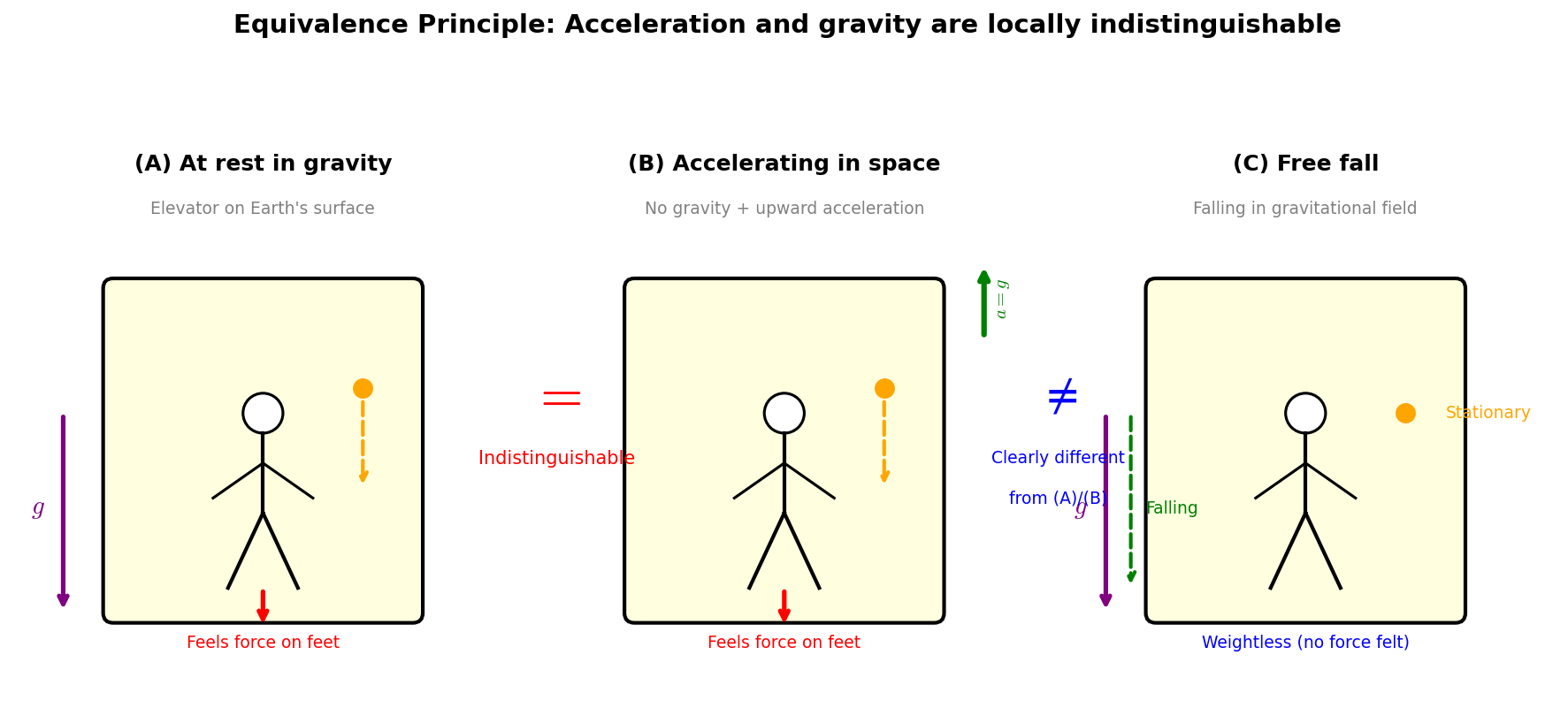
Fig. 6.2: Illustration of the equivalence principle. (A) At rest in a gravitational field and (B) accelerating upward in outer space are locally indistinguishable. (C) In free fall, weightlessness occurs, which is clearly different from (A)/(B).
⚪ Mei: Lina, I'm curious about that "locally" condition—if you look over a large region, wouldn't the gravitational field vary from place to place, making it distinguishable from acceleration?
🟡 Lina: Exactly right. That "inhomogeneity of the gravitational field" is called tidal force. And tidal force is precisely what manifests as spacetime curvature. The components that can be eliminated by a coordinate transformation (first derivatives of the metric = Christoffel symbols) versus those that cannot be eliminated (second derivatives of the metric = Riemann curvature)—this distinction is the mathematical heart of general relativity's structure.
📖 Connection to General Relativity: The equivalence principle, the equivalence of inertial and gravitational mass, the elevator thought experiment in detail, tidal forces, and gravitational redshift (Pound-Rebka experiment) are carefully treated in General Relativity Ch. 5.
✅ Comprehension Check: What is the principle that states acceleration and gravity are locally indistinguishable?
Answer
The equivalence principle. As a consequence, gravity is described not as a "force" but as a geometric property of spacetime.
6.2 Summary of Key Points in General Relativity (What We Need for String Theory)
🟡 Lina: Let's take stock of the tools developed in General Relativity Ch. 5, organized in the form we'll use for string theory.
Unit System in This Chapter
In general relativity, there are many situations where we compare with everyday applications like the Newtonian limit and GPS, so in this chapter we explicitly write \(c\) and use notation closer to SI units. Throughout this book, we use \(c = 1\) (relativity), \(\hbar = c = 1\) (QFT and string theory), or SI units (everyday applications) as appropriate. Refer to the unit conversion table in General Relativity Ch. 4 if needed.
The Metric Tensor \(g_{\mu\nu}\) (General Relativity Ch. 6)
The metric tensor is a generalization of the Minkowski metric \(\eta_{\mu\nu}\) from Ch. 5:
\(g_{\mu\nu}\) is a 4×4 symmetric matrix at each point (\(g_{\mu\nu} = g_{\nu\mu}\), so out of 4×4 = 16 components, the upper and lower triangles are identical, leaving 4 diagonal + 6 upper-triangular = 10 independent components) and is a function of the coordinates. "The measuring rod changes from place to place" is the mathematical expression of "spacetime is curved." In a weak gravitational field, it connects to Newton's gravitational potential \(\Phi\) (at a distance \(r\) from a body of mass \(M\), \(\Phi = -GM/r\), introduced in Ch. 1) via
(the gravitational potential is part of the metric).
🔵 Kai: Wait, Newton's potential directly enters as a component of the metric?
🟡 Lina: Yes. \(g_{00}\) is the "measuring rod" in the time direction. For a clock at rest (\(dx^i = 0\)), only the term \(ds^2 = g_{00}\,c^2 dt^2\) survives from the line element. The signature convention \((-,+,+,+)\) means the signs of the diagonal components of the metric are (time, space, space, space) = (\(-\), \(+\), \(+\), \(+\)). For example, in the Minkowski metric of flat spacetime, \(\eta_{00} = -1\), \(\eta_{11} = \eta_{22} = \eta_{33} = +1\), as we saw in Ch. 5. In the general case too, \(g_{00} < 0\) is maintained, so \(ds^2 = g_{00}\,c^2 dt^2 < 0\)—this is the signature of a "timelike interval."
The proper time \(\tau\) is "the time measured by the clock itself," defined in General Relativity Ch. 4 as \(d\tau^2 = -ds^2/c^2\) (in units where \(c = 1\), \(d\tau^2 = -ds^2\)). In this chapter we use a unit system where \(c\) is explicit, and take coordinates \(x^0 = ct\), \(x^i = (x, y, z)\) (the convention of multiplying the time coordinate by \(c\) to give it dimensions of length—see General Relativity Ch. 4). Since \(x^0 = ct\), the infinitesimal change is \(dx^0 = c\,dt\). Then the line element is \(ds^2 = g_{\mu\nu}\,dx^\mu dx^\nu\), and for a clock at rest (\(dx^i = 0\)), only \(ds^2 = g_{00}\,(dx^0)^2 = g_{00}\,c^2 dt^2\) remains. Here the proper time \(\tau\) is "the time measured by the clock itself," defined as \(d\tau^2 = -ds^2/c^2\) (the minus sign is there because for a timelike worldline \(ds^2 < 0\), so \(-ds^2 > 0\) makes it a positive quantity—see General Relativity Ch. 4). Substituting \(ds^2 = g_{00}\,c^2 dt^2\) gives \(d\tau^2 = -g_{00}\,dt^2\). Since \(g_{00} < 0\), we have \(-g_{00} > 0\), and taking \(d\tau > 0\) (time moves forward) gives \(d\tau = \sqrt{-g_{00}}\,dt\).
⚪ Mei: So in regions where gravity is stronger, \(-g_{00}\) is smaller, and \(d\tau < dt\)—clocks run slow.
🟡 Lina: Exactly. In a weak gravitational field, \(g_{00} \approx -(1 + 2\Phi/c^2)\) with \(|\Phi/c^2| \ll 1\), so \(-g_{00} \approx 1 + 2\Phi/c^2 < 1\) (since \(\Phi < 0\)). When \(0 < -g_{00} < 1\), we have \(\sqrt{-g_{00}} < 1\), so \(d\tau = \sqrt{-g_{00}}\,dt < dt\)—clocks run slower where gravity is stronger (where \(|\Phi|\) is larger). The other components (spatial directions) also change strictly speaking, but in weak gravitational fields the change in \(g_{00}\) dominates.
How much does a clock slow down near the Sun?
At the Sun's surface (\(r = R_\odot \approx 7.0 \times 10^8\) m), substituting \(\Phi = -GM_\odot/r\) into the weak-field approximation \(g_{00} \approx -(1 + 2\Phi/c^2)\) gives \(g_{00} \approx -(1 - 2GM_\odot/(c^2 r))\). Since \(2GM_\odot/c^2 \approx 3.0\) km (corresponding to the Schwarzschild radius \(r_s\) that appears later):
A clock at the Sun's surface runs slower than a distant clock by 4.3 parts per million. For GPS satellites, a similar effect from Earth's gravitational field amounts to 45 microseconds per day. GPS measures distances from the arrival times of radio waves traveling at the speed of light, so a time offset of 45 μs translates to a distance error of \(c \times 45\,\mu\text{s} \approx 3 \times 10^8 \times 45 \times 10^{-6}\,\text{m} \approx 13.5\,\text{km}\)—without correction, position errors of about 10 km per day would accumulate. General relativity is built into everyday technology.
The Geodesic Equation (General Relativity Ch. 8)
🟡 Lina: Objects follow geodesics in curved spacetime—the "straightest possible" paths through spacetime. The equation of motion is
\(\Gamma^\mu_{\alpha\beta}\) are the Christoffel symbols (quantities constructed from first derivatives of the metric \(g_{\mu\nu}\)). Intuitively, they represent "how much the coordinate axes are bending at this location." In a weak gravitational field, \(\Gamma^i_{00} \approx \frac{1}{c^2}\frac{\partial \Phi}{\partial x^i}\), corresponding to Newton's gravitational acceleration \(\mathbf{g} = -\nabla\Phi\). In flat spacetime they are all zero—the relativistic version of Newton's first law. In curved spacetime, \(\Gamma \neq 0\), and the picture is not "being pulled by a force" but rather "following the natural path in curved spacetime."
🔵 Kai: I see—so "falling without feeling gravity" is "natural," and "pushing against gravity with a rocket" is "unnatural."
🟡 Lina: Precisely. Conversely, an object that remains stationary by rocket thrust against gravity is "deviating from a geodesic"—it is the one that's accelerating (Fig. 6.3 "The concept of geodesics").
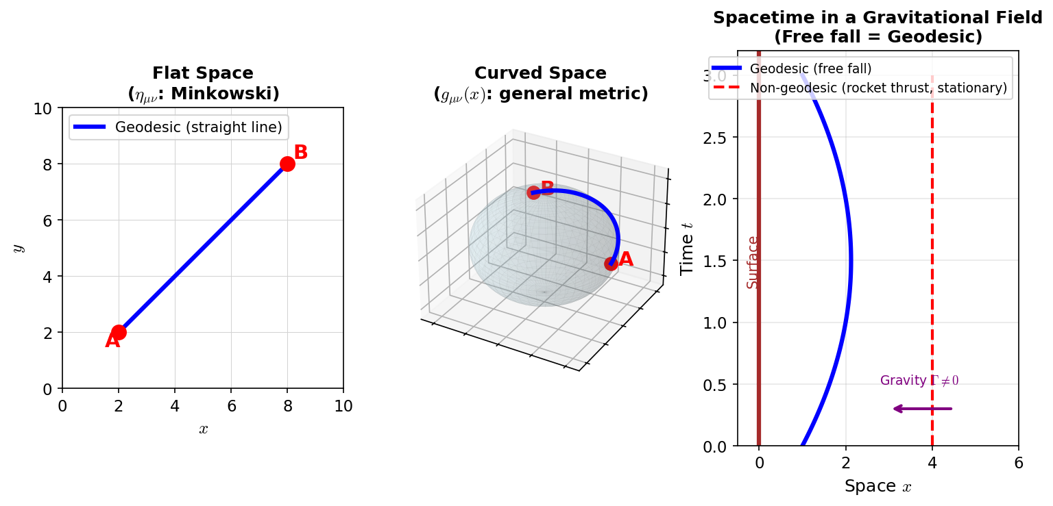
Fig. 6.3: The concept of geodesics. Left: In flat space, the shortest path is a straight line. Middle: On a sphere, great circles are geodesics. Right: In a spacetime diagram with a gravitational field, a freely falling object follows a geodesic, while an object held stationary by rocket thrust deviates from the geodesic.
Curvature and the Riemann Tensor (General Relativity Ch. 13)
The quantity that measures "genuine curvature that cannot be removed by coordinate transformation" is the Riemann curvature tensor \(R^\rho{}_{\sigma\mu\nu}\) (second derivatives of the metric). Intuitively, it measures "the amount by which an arrow (vector) rotates when you carry it around a closed loop on a curved surface while keeping its direction unchanged along the way (this is called parallel transport)." For example, place a northward-pointing arrow at the North Pole of a globe, carry it along a meridian to the equator, move it 90° east along the equator, and carry it back along a meridian to the North Pole—the arrow has rotated 90° from its starting direction. This never happens on a flat surface, so it's evidence of "curvature." In 4 dimensions, symmetry constraints reduce the independent components to 20 (a tensor with 4 indices nominally has \(4^4 = 256\) components, but many symmetries—such as "swapping the first two indices flips the sign" and "exchanging the first pair with the second pair leaves the value unchanged"—drastically reduce this number. See General Relativity Ch. 13 for details. Here, just take away the result "20 components").
🔵 Kai: 256 components reduced to 20… symmetry is powerful.
🟡 Lina: Indeed. Then by contraction—the operation of "choosing a pair of indices and summing them up"—we compress the information into the Ricci tensor \(R_{\mu\nu}\) and the scalar curvature \(R\). Contraction means placing the same index in upper and lower positions and summing from 0 to 3 (Einstein's summation convention introduced in Ch. 5). As a reminder, \(A^\mu B_\mu = A^0 B_0 + A^1 B_1 + A^2 B_2 + A^3 B_3\)—whenever the same letter appears in both upper and lower positions, you automatically sum. Specifically:
In the right-hand side \(R^\lambda{}_{\mu\lambda\nu}\), \(\lambda\) appears in both upper (1st position) and lower (3rd position)—this is a concrete example of "summing over \(\lambda\) from 0 to 3." Similarly, in \(R = g^{\mu\nu}R_{\mu\nu}\), both \(\mu\) and \(\nu\) are contracted, reducing a tensor to a scalar (just a number). Here \(g^{\mu\nu}\) is the inverse matrix of the metric \(g_{\mu\nu}\). Just as multiplying a matrix \(A\) by its inverse \(A^{-1}\) gives the identity matrix \(I\), we have \(g^{\mu\alpha}g_{\alpha\nu} = \delta^\mu_\nu\). \(\delta^\mu_\nu\) is the Kronecker delta—equal to 1 when \(\mu = \nu\) and 0 when \(\mu \neq \nu\), which is just the components of the identity matrix. Using \(g^{\mu\nu}\), you can create \(A^\mu = g^{\mu\nu}A_\nu\) from a lower-index tensor \(A_\mu\)—this is called "raising an index."
⚪ Mei: So raising and lowering indices is handled by the inverse matrix \(g^{\mu\nu}\), and contraction takes sums to reduce the rank of a tensor—combining these two operations, we can compress from the 20 components of the Riemann tensor all the way down to a single scalar.
Einstein's Equation (General Relativity Ch. 14)
How spacetime curves is determined by the distribution of matter and energy:
The left side \(G_{\mu\nu} \equiv R_{\mu\nu} - \frac{1}{2}g_{\mu\nu}R\) is the Einstein tensor (the curvature of spacetime), and the right side \(T_{\mu\nu}\) is the energy-momentum tensor (a quantity expressing how much energy, momentum, and pressure exist at each point). In Wheeler's famous words:
Spacetime tells matter how to move; matter tells spacetime how to curve.
🟡 Lina: To organize the tools so far—\(g_{\mu\nu}\) is the "measuring rod," the geodesic equation is "motion on the measuring rod," and Einstein's equation is "how the measuring rod itself is determined." It's a three-layer structure.
⚪ Mei: I see—the equation that determines the measuring rod and the equation for how objects move on that measuring rod exist separately.
🔵 Kai: The left side is spacetime curvature, the right side is matter… so can spacetime curve even without matter? Could there be solutions where \(T_{\mu\nu} = 0\) but the left side isn't zero? Also, how does this equation arise in string theory?
🟡 Lina: Great questions. For the first part—even with \(T_{\mu\nu} = 0\) (vacuum), nontrivial solutions satisfying \(R_{\mu\nu} = 0\) exist. In fact, the Schwarzschild solution coming up shortly is exactly that. Gravitational waves are also a type of vacuum solution. Even without matter, spacetime itself can "ripple."
For the connection to string theory—when we examine the massless vibrational modes of the string in Ch. 15, we find a spin-2 mode, and from its low-energy effective action, Einstein's equation is automatically re-derived. General relativity is contained within string theory as an approximation—this is one of the main reasons string theory is seriously considered as a candidate for quantum gravity.
✅ Comprehension Check: Describe the relationship between string theory and Einstein's equation. Why does this serve as evidence supporting string theory as a candidate for quantum gravity?
Answer
Einstein's equation is automatically re-derived from the low-energy effective action of the string's massless vibrational modes (spin-2). This means general relativity is contained within string theory as an approximation, demonstrating that string theory naturally describes gravity.
📖 Returning to previously covered topics: The meaning of the metric tensor is in General Relativity Ch. 6, the variational derivation of the geodesic equation and explicit computation of Christoffel symbols are in General Relativity Ch. 8, the geometric meaning of the Riemann tensor is in General Relativity Ch. 13, and the derivation of Einstein's equation from the Einstein-Hilbert action by variation, along with the Einstein–Hilbert priority dispute, is in General Relativity Ch. 14.
✅ Comprehension Check: In general relativity, what is "gravity" described as?
Answer
The curvature of spacetime (the position-dependent variation of the metric tensor \(g_{\mu\nu}\)). Particles are not subject to a force; they move along geodesics of curved spacetime.
6.3 From the Particle Action to the String Action — Enter the Useful Action
🟡 Lina: Now for the original content of this chapter. In the derivation process of the geodesic equation in general relativity, there lies an important structure that extends directly to string theory (Ch. 13). Let's first confirm the form of the particle action, then look at the extension to strings.
The Particle Action: Length of the Worldline
🟡 Lina: When a particle of mass \(m\) moves through curved spacetime, its action is proportional to the integral of proper time along the worldline—that is, the length of the worldline:
Here \(\lambda\) is an arbitrary parameter specifying the worldline—the same idea as parameterizing a curve as \((x(t), y(t))\) with parameter \(t\) in high school math, serving as a label to identify "which point" on the worldline (a general parameter, not necessarily proper time). For a timelike worldline, \(g_{\mu\nu}dx^\mu dx^\nu < 0\) (under the signature convention \((-,+,+,+)\)), so \(-g_{\mu\nu}dx^\mu dx^\nu > 0\) and the square root is well-defined. Here we define \(ds \equiv \sqrt{-g_{\mu\nu}dx^\mu dx^\nu}\) (some conventions write \(ds^2 = -g_{\mu\nu}dx^\mu dx^\nu\)). In particular, when we choose \(\lambda\) to be the proper time \(\tau\), we get \(ds = c\,d\tau\). This action gives the same value regardless of the choice of \(\lambda\) (reparameterization invariance). Varying this action yields the geodesic equation (see General Relativity Ch. 8).
🔵 Kai: That square root looks like it would make calculations messy.
The Useful Action: An Equivalent Form Without the Square Root
🟡 Lina: So we'd like to avoid the square root. The idea is simple: "What if we just use the integrand inside the square root as the Lagrangian—would that give the same path?" The upshot is that there exists an equivalent action that gives the same geodesic but has no square root. However, one additional condition is needed: "choose the parameter \(\tau\) to be proper time"—I'll explain what this means after the formula:
(The original integrand inside the square root was \(-g_{\mu\nu}\dot{x}^\mu\dot{x}^\nu\), but for a timelike worldline \(g_{\mu\nu}\dot{x}^\mu\dot{x}^\nu < 0\), so \(-g_{\mu\nu}\dot{x}^\mu\dot{x}^\nu > 0\). Here we use \(g_{\mu\nu}\dot{x}^\mu\dot{x}^\nu\) directly as the integrand with an overall prefactor \(m/2 > 0\). The sign difference doesn't affect the solutions of the stationarity condition.)
This action has a different form from the original \(S_{\text{particle}}\) (no square root), but it can be shown to give the same geodesic. First, regarding the prefactors \(m\) and \(c\)—multiplying the entire action by a constant doesn't change "the path where the action is stationary." Since the path shape is determined by the condition \(\delta S = 0\), constant multiples are irrelevant. For example, the path that minimizes \(S\) and the path that minimizes \(3S\) are the same, right? So \(m\) is often omitted, but here we keep it to make the correspondence with the string action easier to see later.
⚪ Mei: So \(m\) only sets the "scale" of the action and doesn't affect the shape of the path.
🟡 Lina: Exactly. Next, regarding the absence of the square root—varying this action yields the geodesic equation. Furthermore, the integrand of this action (the quantity corresponding to the Lagrangian) does not explicitly depend on \(\tau\) itself (\(\tau\) doesn't appear directly in the formula; it enters only through \(x^\mu(\tau)\)). In high school physics, you learned that "if the only forces are conservative, energy is conserved." That's actually a special case of a more general principle: "if the laws of the system don't change with time, there exists a conserved quantity." The same applies here—looking at the integrand \(\frac{m}{2}g_{\mu\nu}(x)\dot{x}^\mu\dot{x}^\nu\) of \(S_{\text{useful}}\), \(g_{\mu\nu}\) is a function of \(x\), and \(\dot{x}^\mu\) is also a function of \(x\) and \(\tau\), but there is no term where \(\tau\) itself appears directly (like \(\tau^2\) or \(\sin\tau\)). In such cases—when the Lagrangian does not explicitly contain \(\tau\) (meaning "the laws are the same at every point in \(\tau\)")—a quantity that doesn't change along the equations of motion (a constant of motion) automatically exists.
🔵 Kai: This is the generalization of energy conservation from Ch. 1, right? "If time doesn't appear directly, there's a conserved quantity"—that argument works here too.
🟡 Lina: Precisely. In Ch. 1 you learned "time translation symmetry → energy conservation." There, the conserved quantity had the form \(H = p\dot{q} - L\). The same logic applies here, with \(\tau\) playing the role of time, so a conserved quantity emerges. The Lagrangian of \(S_{\text{useful}}\) is \(L = \frac{m}{2}g_{\mu\nu}\dot{x}^\mu\dot{x}^\nu\), which is a homogeneous quadratic form in \(\dot{x}^\mu\)—meaning every term contains exactly two factors of \(\dot{x}\) (like \(g_{00}(\dot{x}^0)^2\) or \(g_{01}\dot{x}^0\dot{x}^1\); there are no terms with only one \(\dot{x}\) or no \(\dot{x}\) at all). Recall the definition of canonical momentum from Ch. 1—it was \(p = \partial L/\partial\dot{q}\). Here we have 4 coordinates (\(x^0, x^1, x^2, x^3\)), so for each component we define \(p_\mu = \partial L/\partial\dot{x}^\mu\). When differentiating \(L = \frac{m}{2}g_{\alpha\beta}\dot{x}^\alpha\dot{x}^\beta\) with respect to \(\dot{x}^\mu\), the terms in the sum containing \(\dot{x}^\mu\) come from \(\alpha = \mu\) and \(\beta = \mu\)—two contributions. Due to the symmetry of \(g_{\alpha\beta}\) (\(g_{\alpha\beta} = g_{\beta\alpha}\)), these two contributions have the same value, so together they produce a factor of 2 that cancels the \(\frac{1}{2}\) in front, giving \(p_\mu = m\,g_{\mu\nu}\dot{x}^\nu\) (summed over \(\nu\)). (See General Relativity Ch. 8 for calculation details.) Then \(p_\mu\dot{x}^\mu = m\,g_{\mu\nu}\dot{x}^\mu\dot{x}^\nu = 2L\). The conserved quantity formula from Ch. 1 was \(H = p\dot{q} - L\). With 4 coordinates, this extends to \(H = p_\mu\dot{x}^\mu - L\) (summed over \(\mu\) from 0 to 3). Substituting gives \(H = 2L - L = L\)—that is, \(L = \frac{m}{2}g_{\mu\nu}\dot{x}^\mu\dot{x}^\nu\) is constant (see General Relativity Ch. 8 for the rigorous derivation). So the constant of motion in this case is:
🔵 Kai: Oh, that comes out beautifully—\(H = 2L - L = L\), so the Lagrangian itself becomes the conserved quantity.
🟡 Lina: This emerges automatically. Choosing this constant to be \(-c^2\) corresponds to "taking \(\tau\) to be proper time." With this choice, it can be shown that the same geodesics as the original square-root action are obtained. Intuitively, under proper-time parameterization, \(g_{\mu\nu}\dot{x}^\mu\dot{x}^\nu = -c^2\) (constant) holds. Then the integrand of the original action \(\sqrt{-g_{\mu\nu}\dot{x}^\mu\dot{x}^\nu} = c\) is also constant, so when varying we don't need to worry about "the effect of the square root's argument changing," and consequently we get the same Euler-Lagrange equation (= geodesic equation) as from the useful action \(S_{\text{useful}}\). In General Relativity Ch. 8, this fact is treated using the convention that "choosing \(\tau\) to be proper time makes the expression under the square root the constant \(L=1\)."
⚪ Mei: So both actions give the same path (geodesic), but the useful action requires the additional convention of setting the scale of \(\tau\) to match proper time.
🔵 Kai: If that extra convention is needed, is it really "useful"?
🟡 Lina: Removing the square root makes variational calculations dramatically easier. One additional parameter convention is a small price to pay.
🔵 Kai: Trading away the square root for a parameter convention… it's debatable whether that's a net gain. But is this form only relevant for this chapter? Or does it come back later?
🟡 Lina: Great question. The key point is that this useful form of the action generalizes directly to string theory.
Extension to Strings (Preview of Chapter 13)
🟡 Lina: When we go from a point particle to a string, the "worldline" becomes a "worldsheet," and "length" becomes "area." The natural action is the Nambu-Goto action—the area of the worldsheet:
Here \(\int d^2\sigma\) is the 2-dimensional integral over the worldsheet (\(\int d\tau\,d\sigma\)). \(\det\) is the determinant (for a 2×2 matrix \(\begin{pmatrix}a & b\\c & d\end{pmatrix}\), it's \(ad - bc\)). \(T\) is the string tension—the energy per unit length of the string (a constant representing how "resistant to stretching" the string is, with the same dimensions as the tension of an everyday thread). \(\sigma^a = (\tau, \sigma)\) are the two parameters of the worldsheet, and \(X^\mu(\sigma^a)\) is the string's position in spacetime. Note: The \(\tau\) and \(\sigma\) here are the two parameters of the worldsheet, distinct from the proper time \(\tau\) used for the particle's worldline in the previous section—same symbols but different context. Here the notation \(\partial_a X^\mu \equiv \partial X^\mu/\partial\sigma^a\) appears, which denotes a partial derivative—\(X^\mu\) depends on two variables \(\tau\) and \(\sigma\), and we differentiate with respect to only one (say \(\tau\)) while holding the other (\(\sigma\)) fixed. The \(dx/dt\) you learned in high school is differentiation when there's only one variable; when there are multiple variables, "differentiating with respect to only one while keeping the others fixed" is partial differentiation. We use the symbol \(\partial\) (round d) to distinguish it from the ordinary \(d\).
🔵 Kai: For the particle there was 1 parameter (\(\tau\)), but for the string there are 2 (\(\tau, \sigma\)), so partial derivatives become necessary.
🟡 Lina: Exactly. Using this notation, we can write the definition of \(\gamma_{ab}\). From here on, the explanation is about the motivation for "why this quantity appears"—even if you can't follow the index calculations, just take away the conclusion (\(\gamma_{ab}\) is the measuring rod on the worldsheet) and you'll be fine.
Why do we need \(\gamma_{ab}\) separate from \(g_{\mu\nu}\)? Because \(g_{\mu\nu}\) is the measuring rod for all of 4-dimensional spacetime, but the string's worldsheet is a 2-dimensional "sheet," so we need to extract only the distances on that 2-dimensional surface. The 4-dimensional spacetime indices \(\mu, \nu\) take values 0 through 3, but the worldsheet is 2-dimensional, so the worldsheet indices \(a, b\) take only two values, 0 and 1 (\(\sigma^0 = \tau\), \(\sigma^1 = \sigma\)). That is, \(\gamma_{ab}\) is a 2×2 matrix.
The definition is \(\gamma_{ab} \equiv \partial_a X^\mu\,\partial_b X^\nu\,g_{\mu\nu}\), called the induced metric. The meaning is straightforward—when we infinitesimally change the parameters on the worldsheet, the string's spacetime position changes by \(dX^\mu = \partial_a X^\mu\,d\sigma^a\) (with the summation convention over \(a\), this expands to \(= \frac{\partial X^\mu}{\partial\tau}d\tau + \frac{\partial X^\mu}{\partial\sigma}d\sigma\)), so the distance on the worldsheet measured with the spacetime metric is
Expanding: \(ds^2_{\text{worldsheet}} = \gamma_{00}\,d\tau^2 + 2\gamma_{01}\,d\tau\,d\sigma + \gamma_{11}\,d\sigma^2\), where \(\gamma_{00}\) is "the squared spacetime distance when moving slightly in the \(\tau\) direction," \(\gamma_{11}\) is "the squared spacetime distance when moving slightly in the \(\sigma\) direction," and \(\gamma_{01}\) is "the cross term when the two directions aren't orthogonal"—exactly the same structure as how the 4-dimensional \(g_{\mu\nu}\) determined distances in each direction, now shrunk down to 2 dimensions. In other words, \(\gamma_{ab}\) is "the measuring rod on the worldsheet"—the 4-dimensional measuring rod \(g_{\mu\nu}\) restricted to the 2-dimensional surface. \(\sqrt{-\det(\gamma_{ab})}\) gives the area element of the worldsheet. Details are treated carefully in Ch. 13. Like the particle's square-root action, this form is also unwieldy.
So using the same idea as for the particle, we use an equivalent action without the square root—the Polyakov action:
Here \(h_{ab}\) is an auxiliary 2×2 metric introduced on the worldsheet—a "tool" that makes the formula easier to handle without adding physical degrees of freedom. It may seem strange that introducing a new variable doesn't add degrees of freedom, but the equation of motion for \(h_{ab}\) itself (obtained by varying \(S_P\) with respect to \(h_{ab}\)) demands \(h_{ab} = \gamma_{ab}\), so \(h_{ab}\) is not an independent degree of freedom—it's completely determined by the other variables. Just as for the particle we "removed the square root at the cost of a parameter convention," for the string we introduce \(h_{ab}\) and gain an equation-of-motion constraint in return—but the benefit of eliminating the square root outweighs this. \(h^{ab}\) is its inverse matrix, and \(h = \det(h_{ab})\) is its determinant. Since the worldsheet also has a time direction, \(h_{ab}\) has Minkowski-like signature, and the determinant \(h\) is negative—so we take \(-h > 0\) and write \(\sqrt{-h}\) (for the same reason we write \(\sqrt{-g}\) for the 4-dimensional \(g_{\mu\nu}\)). \(\sqrt{-h}\) is the factor that correctly measures "area elements" on the worldsheet. Solving the equation of motion for \(h_{ab}\) yields the condition \(h_{ab} = \gamma_{ab}\); substituting this back recovers the original Nambu-Goto action—so the square root was removed at the cost of one condition, but the physical content is the same. And because there's no square root, quantization becomes possible.
🔵 Kai: The structure looks exactly like the particle's \(S_{\text{useful}} = \frac{m}{2}\int d\tau\,g_{\mu\nu}\dot{x}^\mu\dot{x}^\nu\). But for the particle the mass \(m\) appeared in front, while for the string it's changed to tension \(T\)—aren't mass and tension physically completely different things?
🟡 Lina: Good eye. The particle's mass \(m\) is "resistance to motion," while the string's tension \(T\) is "resistance to stretching"—their physical meanings are indeed different. But within the structure of the action, both sit in the same position as "the constant that determines the inertia of motion." We'll look at this more deeply in Ch. 13. Structurally it's exactly the same idea—the extension from point particle → string is just the replacement of "worldline length" with "worldsheet area," and \(\dot{x}^\mu \dot{x}^\nu\) with \(\partial_a X^\mu \partial_b X^\nu\). The useful-action technique from general relativity is reused directly in string theory—this is the skeleton of the string action that we'll treat in detail in Ch. 13 (Fig. 6.4 "Extension from point particle to string").
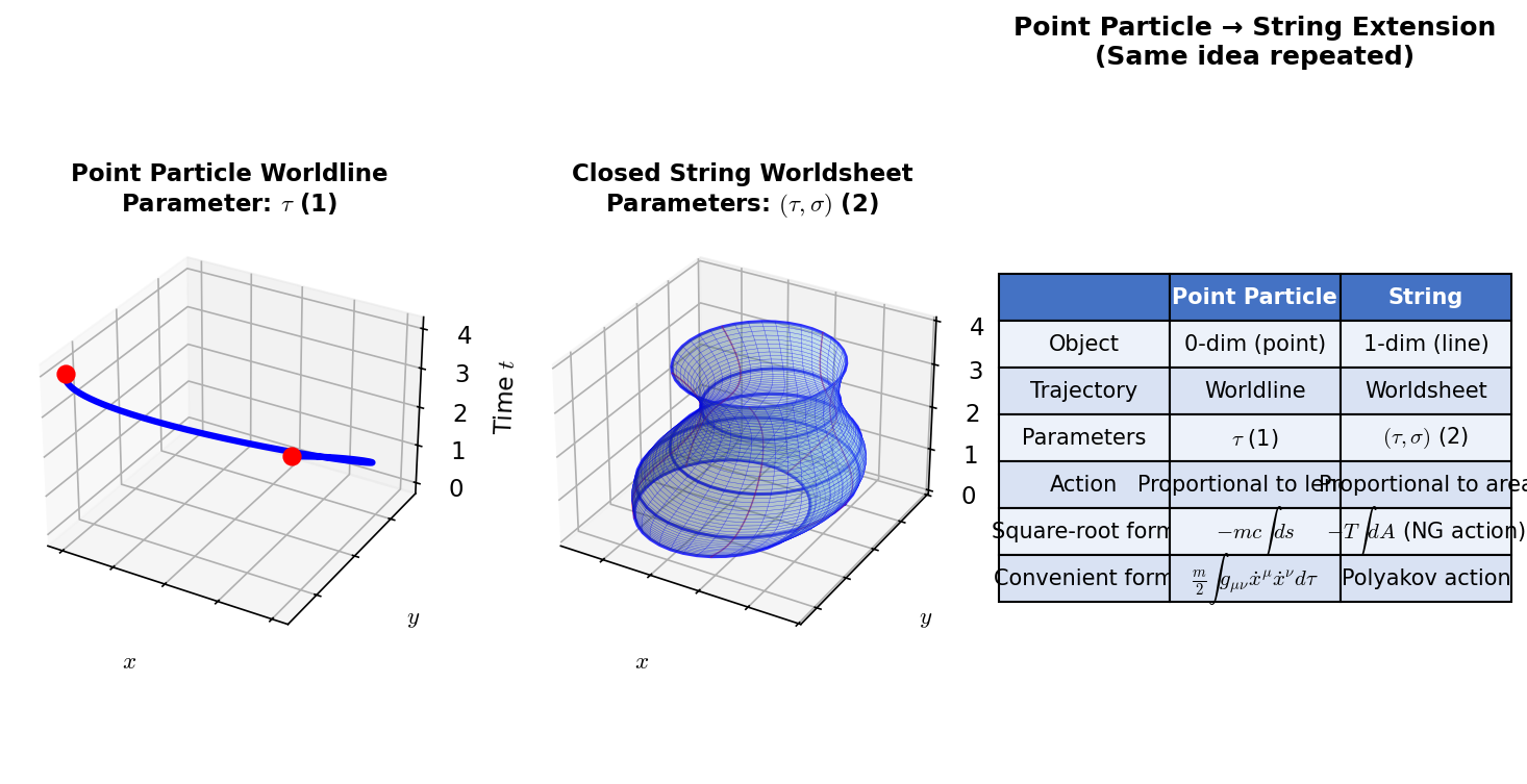
Fig. 6.4: Extension from point particle to string. Left: Point particle's worldline (1 parameter \(\tau\)). Middle: Closed string's worldsheet (2 parameters \((\tau, \sigma)\)). Right: Summary of correspondences. The same idea (removing the square root) is used repeatedly.
🟡 Lina: The action principle as a common language runs in a single thread from Newtonian mechanics (Ch. 1) through general relativity to string theory. In Newtonian mechanics \(S = \int L\,dt\), for the relativistic point particle \(S = -mc\int ds\) (worldline length), and for the string \(S_{\text{NG}} = -T\int dA\) (worldsheet area)—as the dimension of the object increases, we extend from "length → area," but the principle of "making the action stationary" remains the same throughout. Only "what volume we're measuring" changes; the framework of the variational principle itself is invariant.
⚪ Mei: I see—for particles it's length, for strings it's area, but the skeleton of "making the action stationary" is the same throughout.
Table 6.1: Unified structure of the action principle: From Newtonian mechanics to string theory
| Object | Dimension | Trajectory | Action (geometric) | Action (useful form) |
|---|---|---|---|---|
| Newtonian particle | 0 | Orbit \(x(t)\) | \(\int L\,dt\) | \(\int \frac{1}{2}m\dot{x}^2 dt\) |
| Relativistic particle | 0 | Worldline | \(-mc\int ds\) (length) | \(\frac{m}{2}\int g_{\mu\nu}\dot{x}^\mu\dot{x}^\nu d\tau\) |
| String | 1 | Worldsheet | \(-T\int dA\) (area, NG) | Polyakov action (introduce \(h_{ab}\)) |
| Membrane (p-brane) | \(p\) | Worldvolume | \(-T_p\int d^{p+1}\text{Vol}\) | (appears in superstring theory) |
📖 Connection to General Relativity: The detailed derivation of the geodesic equation including Christoffel symbols from the particle's square-root action is in General Relativity Ch. 8. The trick of choosing proper time as the parameter is treated in the same chapter.
✅ Comprehension Check: How is the particle's "useful action" \(S_{\text{useful}} = \frac{m}{2}\int d\tau\,g_{\mu\nu}\dot{x}^\mu\dot{x}^\nu\) extended in string theory?
Answer
Through the replacements worldline → worldsheet, \(\dot{x}^\mu\dot{x}^\nu \to \partial_a X^\mu\partial_b X^\nu\), it extends to the Polyakov action. The advantage of having no square root and enabling quantization is the same. Details are treated in Ch. 13.
6.4 The Schwarzschild Solution and Mercury's Perihelion Precession (Results Only)
🟡 Lina: Solving Einstein's equation for spherical symmetry in vacuum (\(T_{\mu\nu} = 0\)) yields the Schwarzschild metric:
Here \((r, \theta, \phi)\) are spherical coordinates—\(r\) is the distance from the center, \(\theta\) is the angle from the north pole (\(0\) to \(\pi\)), and \(\phi\) is the longitudinal angle (\(0\) to \(2\pi\)). The part \(r^2(d\theta^2 + \sin^2\theta\,d\phi^2)\) represents how distances are measured on a sphere. \(r_s = 2GM/c^2\) is the Schwarzschild radius (the same quantity that appeared in Ch. 4—from this chapter onward we use \(r_s\) to match the standard notation of general relativity). This plays an important role in string theory as well—it reappears throughout, including the D-brane black hole solutions of Ch. 10, the black hole thermodynamics of Ch. 18, and the black hole information paradox of Ch. 20.
🔵 Kai: It looks like \(g_{00}\) goes to zero and \(g_{rr}\) diverges at \(r = r_s\)—what happens there?
🟡 Lina: Good observation. \(r = r_s\) is called the event horizon, and it appears to be a singularity, but it's actually just a divergence due to the choice of coordinates—switching to different coordinates (such as Eddington-Finkelstein coordinates) allows smooth passage through it. The real singularity is at \(r = 0\)—we'll see that shortly.
✅ Comprehension Check: Under what conditions is the Schwarzschild metric obtained as a solution to Einstein's equation? What is the definition of the Schwarzschild radius \(r_s\)?
Answer
It's the result of solving under the conditions of spherical symmetry and vacuum (\(T_{\mu\nu} = 0\)). The Schwarzschild radius is defined as \(r_s = 2GM/c^2\) and gives the characteristic scale for a body of mass \(M\).
Mercury's Perihelion Precession
🟡 Lina: Using perturbation expansion (a method of systematically calculating deviations from Newtonian mechanics as small corrections) on the geodesic equation in the Schwarzschild metric, one can show that the perihelion—the point in an elliptical orbit closest to the Sun—rotates slightly each revolution. Here \(a\) is the semi-major axis (the longer radius of the ellipse) and \(e\) is the eccentricity (a measure of how elongated the ellipse is: 0 for a circle, approaching 1 for very elongated). Using the semi-latus rectum \(p = a(1-e^2)\), the rotation angle is:
(Fig. 6.5 "Mercury's perihelion precession"). Let's substitute Mercury's orbital elements (\(a = 5.79 \times 10^{10}\) m, \(e = 0.2056\), period \(\approx 88\) days). \(p = a(1-e^2) \approx 5.55 \times 10^{10}\) m, and \(GM_\odot/c^2 \approx 1.48 \times 10^3\) m (half the Schwarzschild radius), so per orbit \(\delta\phi = 6\pi \times 1.48 \times 10^3 / (5.55 \times 10^{10}) \approx 5.0 \times 10^{-7}\) rad.
⚪ Mei: Per orbit it's a tiny angle, but it accumulates over time.
🟡 Lina: Right. A century is about 415 orbits, so \(415 \times 5.0 \times 10^{-7} \approx 2.1 \times 10^{-4}\) rad \(\approx 43\) arcseconds—in perfect agreement with the observed value, with no adjustable parameters. Einstein himself said that upon obtaining this result, "his heart was pounding."
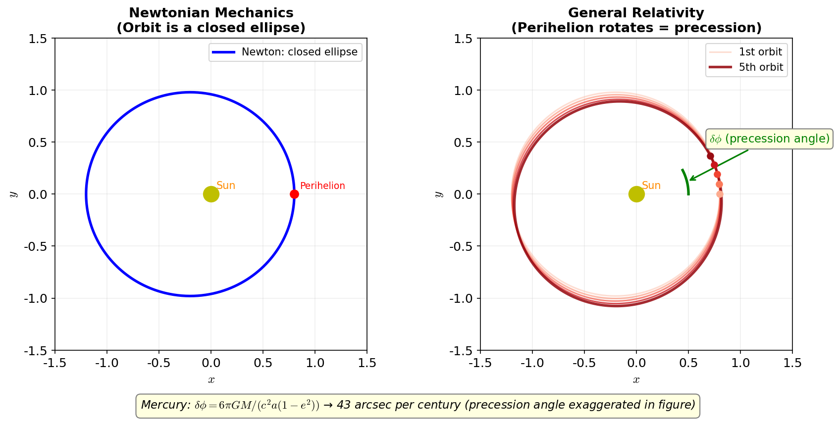
Fig. 6.5: Mercury's perihelion precession. Left: In Newtonian mechanics, the orbit is a closed ellipse. Right: In general relativity, the major axis of the ellipse (direction of perihelion) rotates slightly with each orbit (precession). The precession angle is exaggerated in the figure.
🔵 Kai: Getting exactly 43 arcseconds with no adjustable parameters is incredible… But conversely, if the observed value weren't 43 arcseconds, general relativity would be immediately ruled out?
🟡 Lina: Precisely. Having no additional parameters means that if the observation didn't match, the theory would be immediately falsified—the essence of "falsifiability" from the Prologue. This was general relativity's first experimental triumph and one of the grounds for why the current model is treated as "the best hypothesis."
📖 Connection to General Relativity: The derivation of the Schwarzschild metric is in General Relativity Ch. 9. The perturbation calculations and numerical evaluations of Mercury's perihelion precession, light deflection, and Shapiro delay are treated in detail in General Relativity Ch. 10.
✅ Comprehension Check: In the general relativistic prediction of Mercury's perihelion precession \(\delta\phi = 6\pi GM/[c^2 a(1-e^2)]\), what does "no adjustable parameters" mean?
Answer
\(G\), \(c\), \(M_\odot\), and Mercury's orbital elements are all independently measured values, and the theory has not a single free constant. If the observed value deviated from the predicted value, general relativity would be immediately falsified. This is the essence of falsifiability.
6.5 The Remaining Question — Singularities and the Gateway to Quantum Gravity
🟡 Lina: The predictions of general relativity have been confirmed one after another—Mercury's perihelion precession, light deflection (1919 solar eclipse observation), GPS time corrections, and gravitational waves. Gravitational waves are ripples in spacetime itself propagating at the speed of light—predicted as vacuum solutions of Einstein's equation, generated by accelerating massive objects (such as orbiting binary systems) (Fig. 6.6 "Gravitational waveform from a binary black hole merger (conceptual diagram of GW150914). Top: Time series of strain \(h(t)\)"). Here's a summary of the main experimental verifications.
Table 6.2: Main experimental verifications of general relativity
| Verification | Era | Predicted Value | Precision |
|---|---|---|---|
| Mercury's perihelion precession | 1915 | 43 arcsec/century | Agreement with no parameters |
| Light deflection | 1919 | 1.75 arcsec (solar limb) | \(10^{-4}\) precision with VLBI |
| Gravitational redshift | 1960 (Pound-Rebka) | \(\Delta f/f = gh/c^2\) | \(10^{-4}\) → \(10^{-14}\) (modern) |
| GPS time correction | 1990s– | 45 \(\mu\)s/day | Built into everyday technology |
| Direct gravitational wave detection | 2015 (LIGO) | Waveform template match | SNR > 24 |
In 2015, LIGO first detected GW150914—a waveform generated by a binary black hole merger (Fig. 6.6 "Gravitational waveform from a binary black hole merger (conceptual diagram of GW150914). Top: Time series of strain \(h(t)\)").
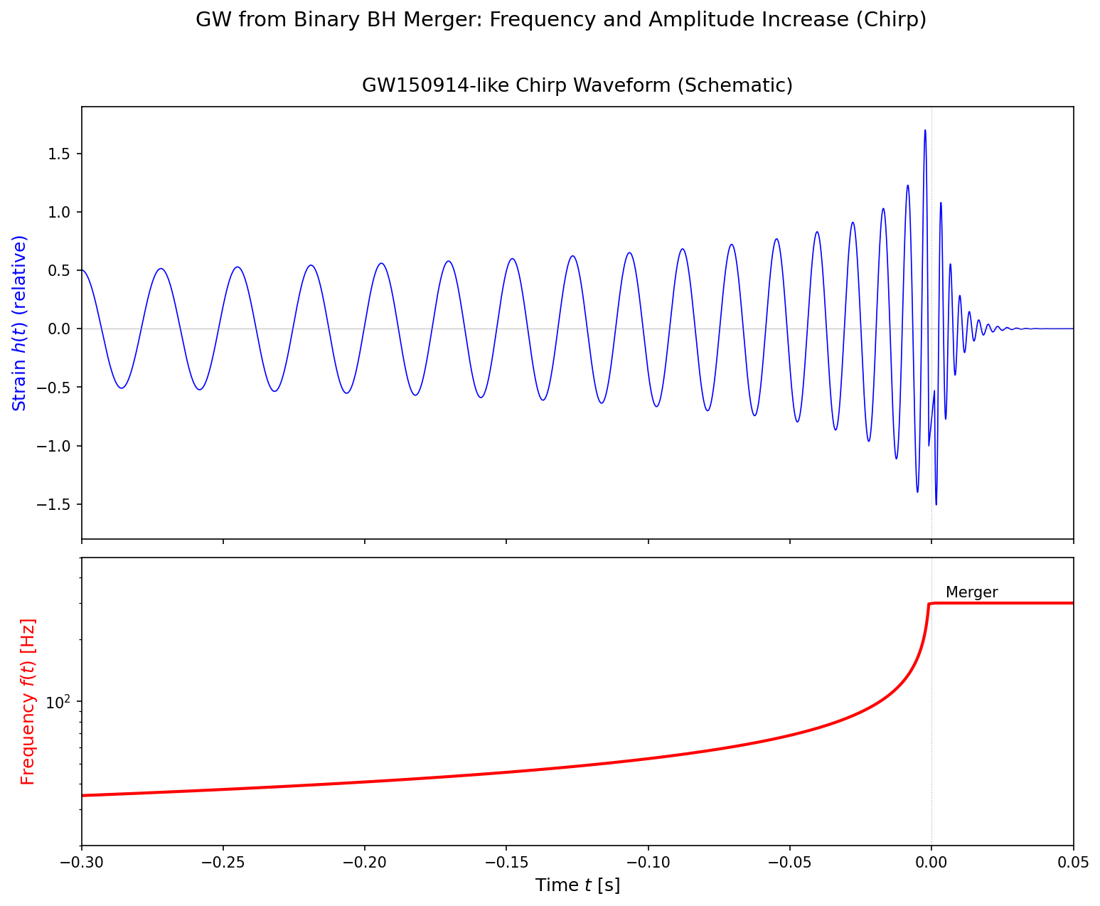
Fig. 6.6: Gravitational waveform from a binary black hole merger (conceptual diagram of GW150914). Top: Time series of strain \(h(t)\)—a "chirp" waveform where amplitude and frequency increase rapidly just before merger. Bottom: Instantaneous frequency \(f(t)\)—during the inspiral phase it follows \(f \propto (t_{\text{merge}} - t)^{-3/8}\), rises to \(\sim 250\) Hz at merger, then rapidly decays (ringdown). The waveform predicted by general relativity matched the LIGO observation through comparison with millions of templates from numerical relativity.
🔵 Kai: What's a chirp? I've heard the name before but…
🟡 Lina: It's a waveform where both amplitude and frequency increase as merger approaches. It's called that because it resembles a bird's chirp. Looking at the bottom panel of Fig. 6.6 "Gravitational waveform from a binary black hole merger (conceptual diagram of GW150914). Top: Time series of strain \(h(t)\)", you can see the frequency rising rapidly before merger—general relativity predicts it follows the power law \(f \propto (t_{\text{merge}} - t)^{-3/8}\). This waveform template and LIGO's observational data matched precisely—this is the most dramatic verification of Einstein's equation. But one serious problem remains.
🔵 Kai: How precisely do they match? If there's even a slight discrepancy, doesn't that mean general relativity is wrong?
🟡 Lina: Compared with millions of templates computed by numerical relativity, they match with a signal-to-noise ratio above 24—meaning the probability of coincidental agreement is negligibly small. If there were a discrepancy, modifications to general relativity would indeed be needed. But for now, the serious problem lies elsewhere.
🔵 Kai: What kind of problem?
🟡 Lina: Singularities.
🔵 Kai: Singularities…? You mean something becomes infinite?
🟡 Lina: Yes. In the Schwarzschild metric at \(r = 0\), a curvature invariant that cannot be removed by coordinate transformation (called the Kretschner scalar—obtained by squaring all components of the Riemann tensor and summing them, a coordinate-independent measure of "the strength of curvature")
diverges. A genuine singularity. The singularity theorems of Penrose and Hawking (1960s) proved that singularity formation is inevitable under very general conditions.
🔵 Kai: So general relativity predicts its own breakdown… But isn't it possible that something different physically happens, even though the math diverges?
🟡 Lina: Good question. The divergence at \(r = r_s\) (the event horizon) is actually due to the choice of coordinates and can be removed by a coordinate transformation—an apparent singularity. But at \(r = 0\), a curvature invariant (a coordinate-independent quantity) diverges, so it cannot be removed by coordinate transformation—a genuine singularity. And near it, the curvature reaches the Planck scale \(\ell_P = \sqrt{\hbar G/c^3} \approx 10^{-35}\) m, where quantum effects can no longer be ignored. This means a theory of quantum gravity unifying general relativity and quantum mechanics is needed—this is the quantum gravity problem addressed in Part III of The Quest for Quantum Gravity (Chapters 10-12).
🔵 Kai: So how does string theory solve this problem?
🟡 Lina: Let me preview just the core idea. A point particle has zero size, so the situation of "infinite energy concentrated at a single point" is unavoidable. But a string has a finite length \(\ell_s \sim 10^{-34}\) m, so even when trying to probe "points" below the Planck scale, the string's extent acts as a natural cutoff. We'll see this in detail in Part IV (Ch. 13 onward).
🔵 Kai: A cutoff… so you mean something like "scales smaller than this can't be seen"? I'm curious whether the singularity disappears or just becomes invisible.
🟡 Lina: Good question. "Cutoff" is a physics term meaning "a boundary below which the theoretical description changes." Your intuition is correct—in string theory, the description of spacetime itself changes at scales below \(\ell_s\), so the situation of "collapsing to a point" simply doesn't occur—the singularity is resolved, not merely hidden. However, the specific mechanism will be seen step by step from Ch. 13 onward.
🔵 Kai: I see… it's not "invisible" but "doesn't happen." But wait—the string length \(\ell_s\) is about the same order as the Planck length \(\ell_P\), right? So wouldn't the string itself get caught up in the singularity?
🟡 Lina: Sharp. \(\ell_s\) and \(\ell_P\) are indeed of similar order, but the point is that the very picture of "the string falling into the singularity" doesn't hold. A point particle can reach the "location" \(r = 0\), but a string has finite extent, so at scales below \(\ell_s\), the spacetime description that defines "\(r = 0\) as a location" is itself rewritten. As an analogy, it's not that the map's resolution is too coarse to draw a "point," but rather the map itself switches to a different kind of map—the "destination to fall into" simply ceases to exist. The specific mechanism will be seen from Ch. 13 onward.
⚪ Mei: To summarize—in point particle theories, "infinite energy concentrated at a point of zero size" makes singularities unavoidable. In string theory, the string length \(\ell_s\) becomes a natural minimum scale, and below it the very concept of a "point" vanishes. So the singularity is "resolved"—not hidden, but the stage on which it would occur ceases to exist.
🟡 Lina: Yes, a perfect summary. Let me also summarize the flow of the entire chapter so far—
⚪ Mei: Starting from the equivalence principle, we arrived at "gravity = geometry of spacetime" and described spacetime dynamics with Einstein's equation. But that equation itself predicts singularities—"its own breakdown." Therefore quantum gravity is needed, and its candidate is string theory—that's the path.
🟡 Lina: A perfect summary. Specifically:
- Ch. 10: Schwarzschild black holes and event horizons
- Ch. 11: Big Bang cosmology and the initial singularity
- Ch. 12: The failure of naive attempts to quantize gravity
- Ch. 13: Introducing strings to avoid ultraviolet divergences
- Ch. 20: Microscopic derivation of black hole entropy via D-branes and the black hole information paradox
A note on philosophy of science: General relativity is not a "law" but a model—merely the best hypothesis that hasn't been experimentally refuted. The appearance of singularities clearly indicates the limits of applicability of this model. It's a signal from physics that a better model (quantum gravity) is needed. Physical models are always provisional and may be replaced by more accurate ones. Never forget to maintain the attitude of thinking for yourself.
📖 Connection to General Relativity: Details on black holes are in General Relativity Ch. 16, cosmology and the Big Bang are in General Relativity Ch. 21, and prospects for quantum gravity are in General Relativity Ch. 25.
✅ Comprehension Check: What happens at \(r = 0\) in the Schwarzschild metric? What does this mean for general relativity?
Answer
A "genuine singularity" appears where the curvature invariant \(R_{\mu\nu\rho\sigma}R^{\mu\nu\rho\sigma}\) diverges. This is a sign of general relativity's own limits of applicability and means that a theory of quantum gravity is needed.
Preview of the Next Chapter
Ch. 7「Why Are Atoms Stable? — The Birth of Quantum Mechanics」 — According to classical electrodynamics, an electron should radiate electromagnetic waves, lose energy, and spiral into the nucleus in an instant. Yet real atoms exist stably. To resolve this fatal contradiction, physics required an entirely new framework—quantum mechanics. We follow the story of its birth. This also serves as a bridge to Quantum Mechanics.
Exercises
For exercises corresponding to this chapter's content, refer to the end-of-chapter problems in each chapter of General Relativity. The correspondence with the string theory action is addressed in the exercises of Ch. 13.
References
- General Relativity Ch. 5 Can acceleration and gravity be distinguished? — Details of the equivalence principle
- General Relativity Ch. 6 — The metric tensor and curved spacetime
- General Relativity Ch. 8 What does 'straight' mean in curved spacetime? — Variational derivation of the geodesic equation
- General Relativity Ch. 9 — Derivation of the Schwarzschild solution
- General Relativity Ch. 10 — Mercury's perihelion precession, light deflection, and Shapiro delay
- General Relativity Ch. 13 — The Riemann curvature tensor
- General Relativity Ch. 14 What equation describes how matter curves spacetime? — Derivation from the Einstein-Hilbert action and the Einstein–Hilbert priority dispute
- General Relativity Ch. 16 — Black holes and singularities
- General Relativity Ch. 25 — The challenge of quantum gravity
- David Tong, Lectures on General Relativity — A modern formulation of general relativity
- Barton Zwiebach, A First Course in String Theory, Ch.3, 6 — Extension from the point particle action to the string action
Feedback on this page
Let us know if something was unclear, incorrect, or could be improved.