Appendix D: Foundations of Group Theory and Symmetry
Story so far: In Appendix C, we learned the foundations of tensors and differential geometry. Tools such as the metric tensor, covariant derivative, and curvature tensor were designed to describe the geometric structure of spacetime. However, physics has another powerful principle beyond geometry—"symmetry." All forces in the Standard Model arise from gauge symmetries, and in string theory, the Virasoro algebra and supersymmetry play essential roles. Let us now develop the language for treating symmetry mathematically—group theory.
Goals of this chapter
- Understand the foundations of group theory—the mathematical tool for describing "symmetry"—starting from the concrete example of rotating an equilateral triangle
- Cover the definition of a group, Lie groups (\(U(1)\), \(SU(2)\), \(SU(3)\)), Lie algebras and commutation relations of generators, the concept of representations, Noether's theorem, gauge symmetry and covariant derivatives, and spontaneous symmetry breaking
- This will enable you to follow the mathematical discussions in Ch. 9 (the Standard Model gauge group), Ch. 16 (Virasoro algebra), and Ch. 17 (supersymmetry)
🟡 Lina: If you encountered "\(SU(3) \times SU(2) \times U(1)\)" in Ch. 9 and thought "What's that?"—start here. We'll begin with the familiar example of rotating an equilateral triangle, so there's no need to be intimidated.
D.1 Why Learn Group Theory? — Symmetry Is the Language of Physics
🟡 Lina: The role of symmetry in physics is overwhelmingly important. Recall from Ch. 2 how Maxwell unified electricity and magnetism. In Ch. 9, we saw that the three forces of the Standard Model arise from "gauge symmetries."
🔵 Kai: It's amazing that just "requiring" a symmetry determines the form of the force. But what exactly is "symmetry"? Does it just mean something like "a beautiful shape"?
🟡 Lina: Good question. Intuitively, it means "physics doesn't change under a certain operation." But to define "doesn't change" precisely, we need a mathematical language. That's group theory.
⚪ Mei: So it's a tool for treating symmetry with "equations" rather than "intuition."
🟡 Lina: Exactly. And using group theory, the following becomes possible:
- Deriving conservation laws from symmetry (Noether's theorem)
- Determining the form of forces from symmetry (the gauge principle)
- Classifying particles by symmetry (representation theory)
- Describing how symmetry breaks (spontaneous symmetry breaking)
🔵 Kai: There are four things? Symmetry is that versatile...
🟡 Lina: In string theory too, group theory appears everywhere—the Virasoro algebra (Ch. 16), supersymmetry algebras (Ch. 17), and duality groups (Ch. 18).
✅ Comprehension Check: Name two things that become possible by using group theory.
Answer
For example, (1) deriving conservation laws from symmetry (Noether's theorem), and (2) determining the form of forces from symmetry (the gauge principle). "Classifying particles by symmetry (representation theory)" and "describing how symmetry breaks (spontaneous symmetry breaking)" are also correct answers.
✅ Comprehension Check: What is the language (tool) for describing symmetry mathematically called?
Answer
Group theory.
D.2 What Is a Group? — "A Collection of Operations"
Starting with a Concrete Example — Rotating an Equilateral Triangle
🟡 Lina: Jumping straight to definitions makes things hard to grasp, so let's start with a concrete example.
Rotate an equilateral triangle about its center (Fig. D.1 "Rotational symmetry of an equilateral triangle"). How many rotations make the triangle "look the same as before"?
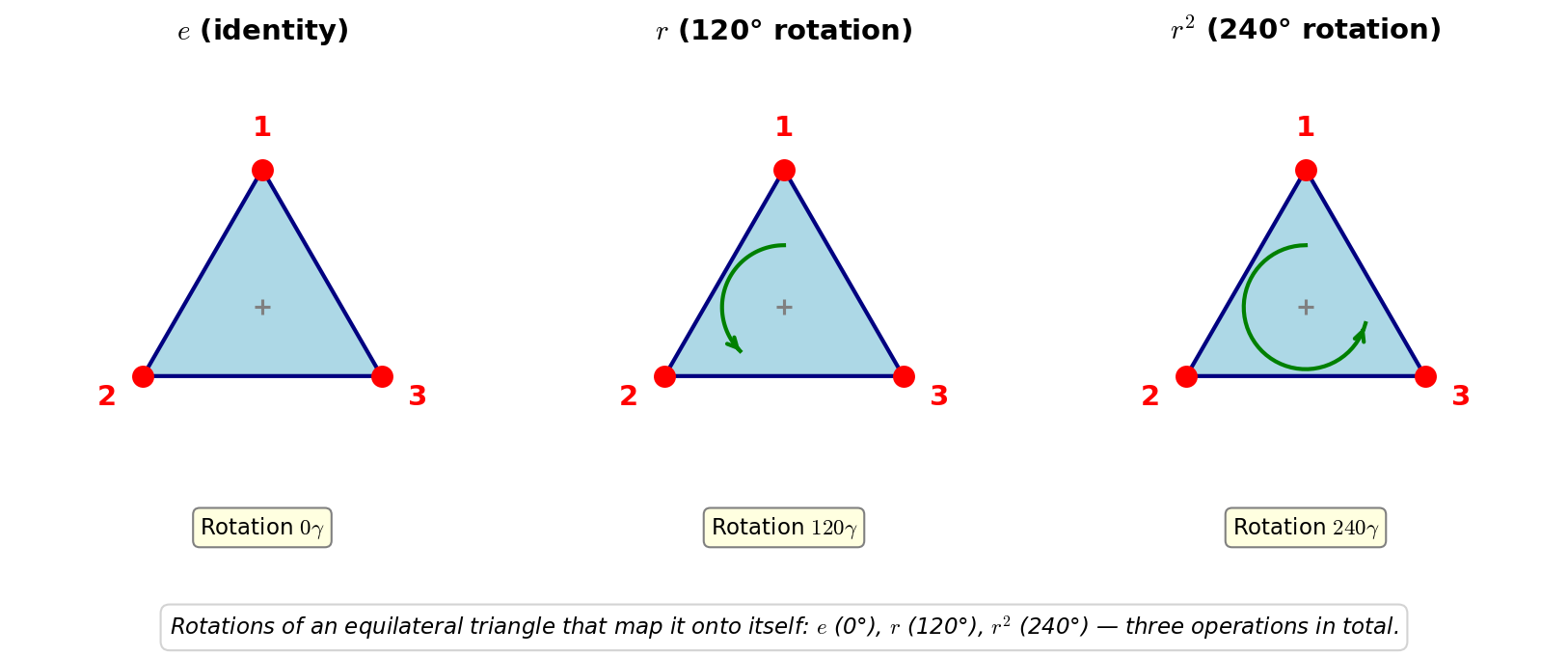
Fig. D.1: Rotational symmetry of an equilateral triangle. Figure D_1: When rotating an equilateral triangle about its central axis, the operations that leave it looking the same are \(e\) (0°), \(r\) (120°), and \(r^2\) (240°).
- No rotation (0°) — we write this as \(e\)
- 120° rotation — we write this as \(r\)
- 240° rotation (= 120° twice) — we write this as \(r^2\)
A 360° rotation returns to the original, so it's the same as \(e\). Thus, the rotations that "make the triangle look the same" are the three elements \(\{e, r, r^2\}\).
🔵 Kai: Only three? A circle would have infinitely many.
🟡 Lina: Yes, that's the difference between a "discrete group" and a "continuous group." We'll get to continuous groups later. First, let's look at the properties of these three operations.
✅ Comprehension Check: How many rotation operations leave an equilateral triangle "looking the same" when rotated about its central axis?
Answer
Three. The 0° rotation (\(e\)), 120° rotation (\(r\)), and 240° rotation (\(r^2\)). A 360° rotation is the same as 0° rotation, so it isn't counted separately.
These three operations have interesting properties:
- Performing two operations in succession always gives one of the three. For example, \(r\) followed by \(r\) gives \(r^2\). \(r\) followed by \(r^2\) gives \(e\) (back to the start). You never leave the set of three.
- When performing three in succession, regrouping doesn't change the result. \((r \cdot r) \cdot r = r^2 \cdot r = e\) and \(r \cdot (r \cdot r) = r \cdot r^2 = e\) are the same.
- There exists a "do nothing" operation \(e\). Doing anything after \(e\), or doing \(e\) after anything, doesn't change the result.
- Every operation has an "undo" operation. The undo of \(r\) is \(r^2\) (doing \(r\) then \(r^2\) gives \(e\)). The undo of \(r^2\) is \(r\).
⚪ Mei: Four properties line up beautifully. These become the conditions for a "group," right?
Written as a multiplication table:
Table D.1: Multiplication table of the cyclic group Z₃
| \(\cdot\) | \(e\) | \(r\) | \(r^2\) |
|---|---|---|---|
| \(e\) | \(e\) | \(r\) | \(r^2\) |
| \(r\) | \(r\) | \(r^2\) | \(e\) |
| \(r^2\) | \(r^2\) | \(e\) | \(r\) |
Definition — Extracting from Concrete Examples
🟡 Lina: The generalization of the four properties above is the definition of a group. When a "collection of operations" \(G\) and a rule \(\cdot\) for performing operations in succession satisfy the following four conditions, we call \((G, \cdot)\) a group:
- Closure: The result \(a \cdot b\) of performing operation \(a\) followed by operation \(b\) is also an operation contained in \(G\)
- Triangle example: \(r \cdot r = r^2 \in \{e, r, r^2\}\) ✓ — never leaves the set of three
- Associativity: \((a \cdot b) \cdot c = a \cdot (b \cdot c)\) — when performing three operations in succession, regrouping doesn't change the result
- Triangle example: \((r \cdot r) \cdot r = r \cdot (r \cdot r) = e\) ✓
- Identity: A "do nothing" operation \(e\) exists (\(e \cdot a = a \cdot e = a\))
- Triangle example: 0° rotation \(e\) ✓
- Inverse: For every operation \(a\), an "undo" operation \(a^{-1}\) exists (\(a \cdot a^{-1} = e\))
- Triangle example: the inverse of \(r\) is \(r^2\) (\(r \cdot r^2 = e\)) ✓
The rotations of the equilateral triangle \(\{e, r, r^2\}\) are called \(\mathbb{Z}_3\) (the cyclic group of order 3).
⚪ Mei: So if even one of the four conditions fails, it's not a group.
🔵 Kai: Associativity basically means "you don't have to worry about the order of computation," right? Like \((1+2)+3 = 1+(2+3)\) in addition.
🟡 Lina: As an example, that's correct. But to be precise, associativity means "changing how you group three elements doesn't change the result." Saying "you don't have to worry about the order" can be confused with "commutativity" (\(a \cdot b = b \cdot a\)), so be careful. Commutativity is about "swapping the order of two elements" and is different from associativity. Commutativity is not a requirement for a group. For example, the natural numbers \(\{1, 2, 3, \ldots\}\) with addition do not form a group. There is no natural number satisfying \(3 + ? = 0\), so the inverse condition is violated.
✅ Comprehension Check: Why don't the natural numbers \(\{1, 2, 3, \ldots\}\) with addition form a group?
Answer
Because inverses don't exist. For example, there is no natural number satisfying \(3 + ? = 0\). The inverse condition among the four group conditions is violated.
Why "Operations"?
🟡 Lina: The key point is to think of a group as "a collection of operations" rather than "a collection of numbers." In physics, a symmetry means "physics doesn't change under a certain operation." The totality of such "operations" forms a group. In the equilateral triangle example, "the triangle looks the same after a 120° rotation" is the symmetry, and the totality of symmetry operations \(\{e, r, r^2\}\) is the group.
📝 Exercises:
✅ Comprehension Check: List the four conditions that constitute the definition of a group.
Answer
Closure, associativity, existence of an identity, and existence of inverses.
✅ Comprehension Check: In the rotation group of the equilateral triangle \(\{e, r, r^2\}\), what is the inverse of \(r\)?
Answer
\(r^2\). Because \(r \cdot r^2 = e\) (returns to the identity).
D.3 Continuous Groups (Lie Groups) — The Stars of Physics
🟡 Lina: The rotations of an equilateral triangle are "discrete" (in 120° steps). But if you rotate a circle, you can rotate by any angle. Groups that are continuously labeled by parameters are called Lie groups. Nearly all the most important groups in physics are Lie groups.
\(U(1)\): Rotation of a Circle — The Symmetry of Electromagnetism
Consider the set of all complex numbers \(e^{i\theta}\) (\(\theta\) is real). The absolute value is always 1 (\(|e^{i\theta}| = 1\)), so this represents rotations on the unit circle in the complex plane.
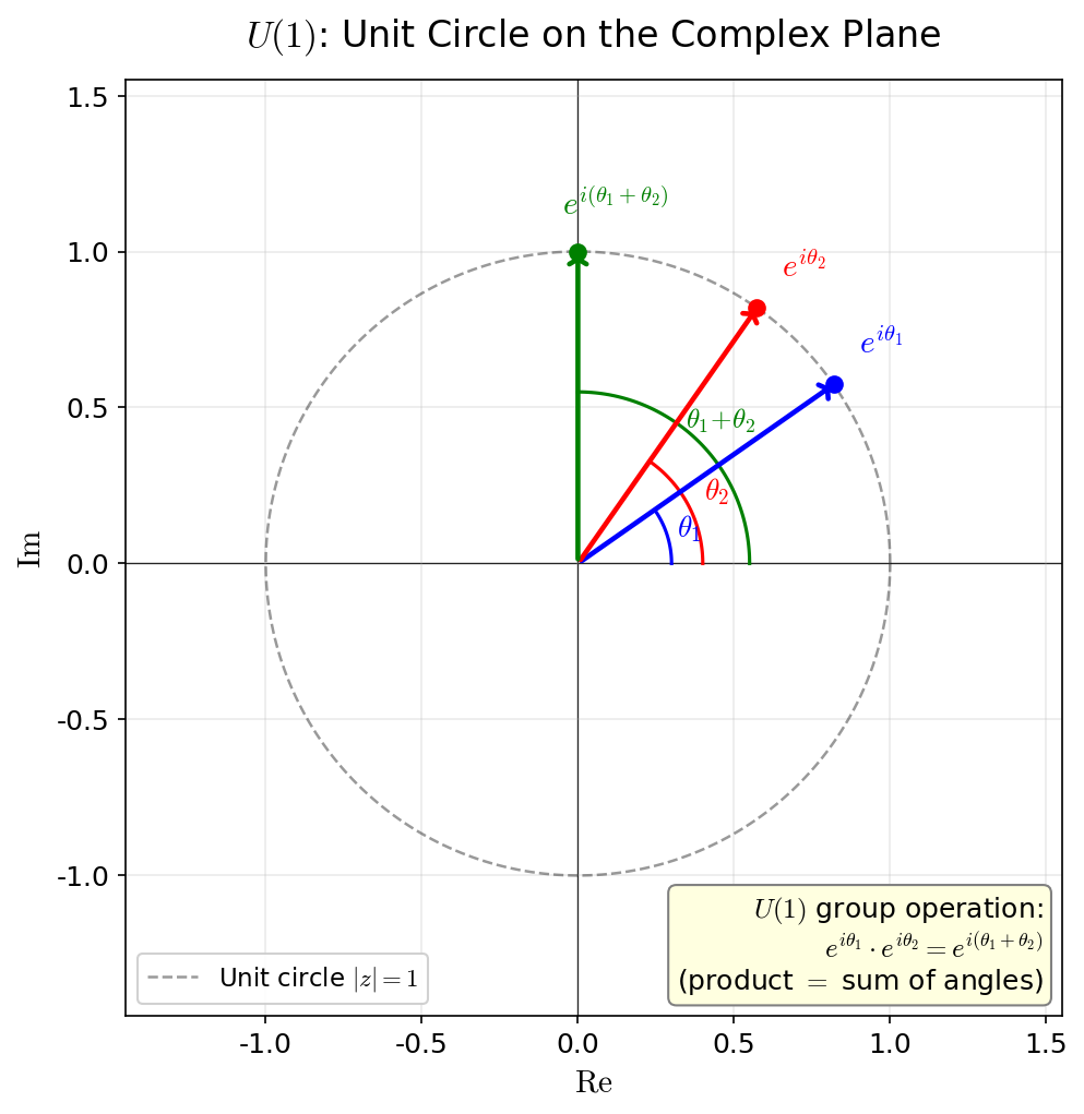
Fig. D.2: The unit circle in the complex plane and U(1). Figure D_2: \(e^{i\theta}\) represents a point on the unit circle in the complex plane. As \(\theta\) varies, the point moves continuously around the circle.
Let's verify the group conditions:
Closure: Compute the product of two elements.
The right side is of the form \(e^{i\theta}\) (\(\theta = \theta_1 + \theta_2\)), so it's contained in \(U(1)\). ✓
Associativity: For three elements,
Both are equal. ✓
Identity: Setting \(\theta = 0\) gives \(e^{i \cdot 0} = 1\). For any element \(e^{i\theta}\), \(1 \cdot e^{i\theta} = e^{i\theta}\). ✓
Inverse: The inverse of \(e^{i\theta}\) is \(e^{-i\theta}\). Verification:
✓
There is only one parameter \(\theta\) → a 1-dimensional Lie group.
🔵 Kai: Oh, all four conditions are verified in one shot. Simple.
✅ Comprehension Check: For which value of \(\theta\) is the \(U(1)\) element \(e^{i\theta}\) the identity of the group? Also, what is the inverse of \(e^{i\theta}\)?
Answer
When \(\theta = 0\), \(e^{i \cdot 0} = 1\) is the identity. The inverse of \(e^{i\theta}\) is \(e^{-i\theta}\) (multiplying gives \(e^0 = 1\)).
🔵 Kai: What does the "\(U\)" in \(U(1)\) stand for?
🟡 Lina: It stands for Unitary. A \(1 \times 1\) unitary matrix is a complex number satisfying \(|u|^2 = 1\), which is precisely \(e^{i\theta}\). So \(U(1)\) is "the group of \(1 \times 1\) unitary matrices."
📝 Exercises:
- Verifying \(U(1)\) group conditions → Problem B-4. Group Conditions of \(U(1)\)
Role in physics (Ch. 9): Consider the phase transformation \(\psi \to e^{i\theta}\psi\) on a quantum mechanical wave function \(\psi\). Requiring that physics doesn't change under this transformation (\(|\psi|^2\) is invariant) causes the photon to automatically appear, and electromagnetism is derived. This is the gauge principle (derived in detail in Section D.7).
\(SO(2)\) and \(SO(3)\): Rotation Groups
🟡 Lina: \(U(1)\) was phase rotation of complex numbers, but the more familiar "spatial rotations" also form a group.
\(SO(2)\): Rotations in 2 dimensions
The matrix that rotates a vector \((x, y)\) by angle \(\theta\) in the 2D plane is:
This is a \(2 \times 2\) orthogonal matrix (\(R^T R = I\)) with determinant 1 (\(\det R = 1\)). The set of all such matrices is \(SO(2)\).
Let's verify closure. The composition of two rotations is:
Computing the matrix product (using addition formulas):
The result is again an element of \(SO(2)\). ✓
🔵 Kai: Wait, both \(SO(2)\) and \(U(1)\) have one parameter and the structure of "adding angles," right? They seem similar.
🟡 Lina: Good observation. In fact, \(SO(2)\) and \(U(1)\) are isomorphic (have the same structure) as groups. There's a correspondence \(e^{i\theta} \leftrightarrow R(\theta)\).
⚪ Mei: So they look different—"phase rotation of complex numbers" versus "rotation matrix in the plane"—but their multiplication structure as groups is exactly the same.
✅ Comprehension Check: What is the relationship between \(SO(2)\) and \(U(1)\)?
Answer
They are isomorphic as groups (have the same structure). There's a correspondence \(e^{i\theta} \leftrightarrow R(\theta)\), and while they look different as "phase rotation of complex numbers" versus "rotation matrix in the plane," their group multiplication structure is exactly the same.
\(SO(3)\): Rotations in 3 dimensions
Rotations in 3D space are represented by \(3 \times 3\) orthogonal matrices (\(R^T R = I\), \(\det R = 1\)). There are 3 parameters (for example, Euler angles \(\alpha, \beta, \gamma\)).
An important property: \(SO(3)\) is non-commutative. That is, the order of rotations matters.
🔵 Kai: If you hold a book, first rotate 90° around the \(x\)-axis, then 90° around the \(z\)-axis, the result is different from doing it in reverse order (Fig. D.3 "Non-commutativity of SO(3) rotations").
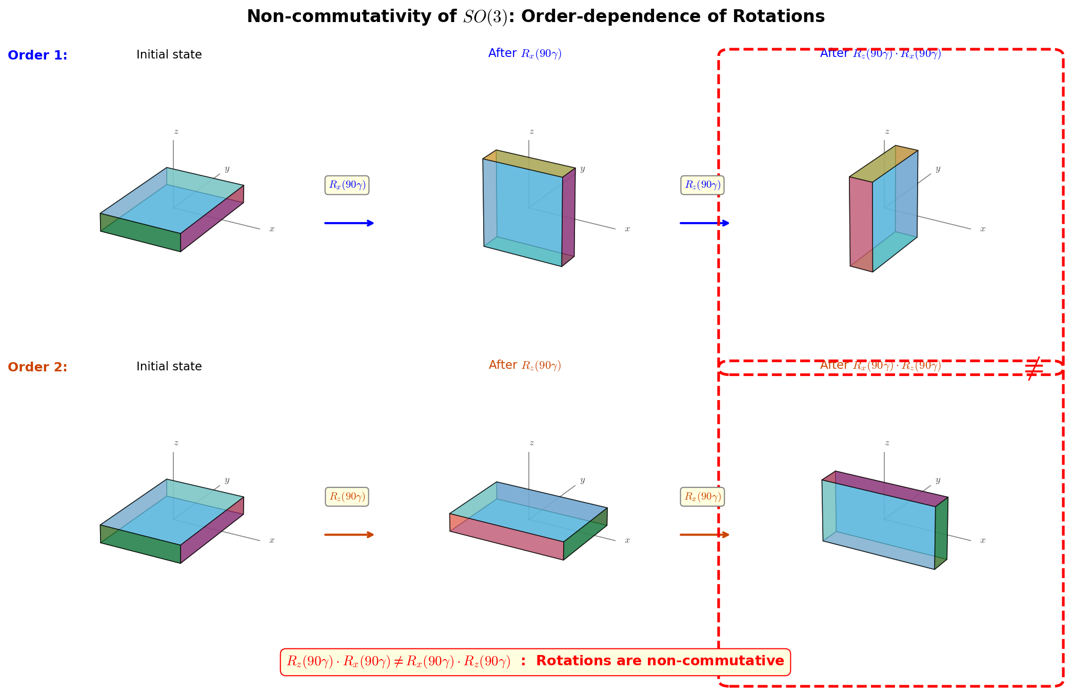
Fig. D.3: Non-commutativity of SO(3) rotations. Figure D_3: Rotations in 3D space give different results when the order is swapped (non-commutative). Rotating a book 90° around the \(x\)-axis then 90° around the \(z\)-axis gives a different result from the reverse order.
🟡 Lina: Exactly. In equations: \(R_x(\pi/2) R_z(\pi/2) \neq R_z(\pi/2) R_x(\pi/2)\). This "order matters" property is the essence of non-commutative groups and the starting point of Yang-Mills theory (Quantum Field Theory Quantum Field Theory Ch. 17).
\(SU(2)\): The Symmetry of the Weak Force
The set of all \(2 \times 2\) unitary matrices (\(U^\dagger U = I\)) with determinant 1 (\(\det U = 1\)).
🔵 Kai: What's "unitary" again?
🟡 Lina: It means the inverse of the matrix equals its conjugate transpose (\(U^{-1} = U^\dagger\)). If you define the "squared length" of a vector \(\mathbf{v} = (v_1, v_2)\) with complex components as \(|v_1|^2 + |v_2|^2\), then multiplying by a unitary matrix doesn't change this length. It's the same idea as how the length \(\sqrt{x^2 + y^2}\) of a real vector is preserved by orthogonal matrices (rotation matrices), extended to complex numbers.
There are 3 parameters → a 3-dimensional Lie group.
🔵 Kai: How do we know it's 3?
🟡 Lina: Let's count. A \(2 \times 2\) complex matrix has 8 real parameters (each entry is complex with a real and imaginary part, giving 2 each, and 4 entries give \(2 \times 4 = 8\)). How many real conditions does the unitarity condition \(U^\dagger U = I\) impose?
🔵 Kai: \(U^\dagger U\) is a \(2 \times 2\) matrix, so each of 4 entries equals the corresponding entry of \(I\)... that's 4 complex number equalities, meaning 8 real conditions?
🟡 Lina: It looks that way at first. But actually \(U^\dagger U\) has a special property. \((U^\dagger U)^\dagger = U^\dagger (U^\dagger)^\dagger = U^\dagger U\), so \(U^\dagger U\) is a Hermitian matrix (satisfying \(H^\dagger = H\)). Since Hermitian matrices have constraints on their entries, the 4 equalities are not all independent.
🔵 Kai: What changes when it's Hermitian?
🟡 Lina: A Hermitian matrix has real diagonal entries (\(H_{ii}^* = H_{ii}\)), and off-diagonal entries satisfy \(H_{ji} = H_{ij}^*\)—they determine each other. So only the upper-triangular entries (\(i < j\)) are independent, giving \(n(n-1)/2\) complex numbers for the off-diagonal part.
🔵 Kai: Ah, so the lower triangle is determined as the complex conjugate of the upper triangle, meaning only half can be freely chosen.
🟡 Lina: Right. For \(n \times n\), there are \(n\) real numbers on the diagonal and \(n(n-1)/2\) independent complex off-diagonal entries (= \(n(n-1)\) real numbers), giving \(n + n(n-1) = n^2\) independent real components for a Hermitian matrix. The equation "\(n \times n\) Hermitian matrix = identity matrix" says each of these \(n^2\) independent real components equals the corresponding entry of the identity (1 on diagonal, 0 off-diagonal), giving \(n^2\) independent real equations. For \(2 \times 2\), that's \(2^2 = 4\). Not 8, but 4.
⚪ Mei: I see, thanks to the Hermitian property, the number of conditions is reduced to less than half.
🔵 Kai: Wait, I understand the conditions are 4 for Hermitian. But "\(\det U = 1\) reduces by 1"—does that mean the determinant condition counts as 1 real number? Isn't the determinant complex?
🟡 Lina: Good question. The determinant of a unitary matrix automatically satisfies \(|\det U| = 1\) (meaning \(\det U = e^{i\theta}\), with absolute value always 1). So \(\det U = 1\) just adds the single real condition "\(\theta = 0\)." Thus \(8 - 4 = 4\), then \(4 - 1 = 3\).
⚪ Mei: So starting from 8 real parameters, the unitarity condition removes 4, the determinant condition removes 1, and 3 remain.
🟡 Lina: Exactly. A general element of \(SU(2)\) can be written as:
Here \(\alpha, \beta\) are complex numbers. Computing the determinant (for a \(2 \times 2\) matrix \(\begin{pmatrix}a&b\\c&d\end{pmatrix}\), the determinant is \(ad - bc\)): \(\det U = \alpha \cdot \alpha^* - (-\beta^*) \cdot \beta = |\alpha|^2 + |\beta|^2 = 1\) ✓. Together \(\alpha\) and \(\beta\) have 4 real parameters, but the condition \(|\alpha|^2 + |\beta|^2 = 1\) removes one, so the independent real parameters are indeed 3.
✅ Comprehension Check: Explain why the number of parameters for \(SU(2)\) is 3, using the counting of conditions.
Answer
A \(2 \times 2\) complex matrix has 8 real parameters. The unitarity condition \(U^\dagger U = I\) imposes 4 real conditions, and \(\det U = 1\) removes one more. Thus \(8 - 4 - 1 = 3\).
📝 Exercises:
- Computing an \(SU(2)\) element concretely from Pauli matrices → Problem M-1. Exponential Representation of \(SU(2)\) Elements
Relationship between \(SU(2)\) and \(SO(3)\):
\(SU(2)\) and \(SO(3)\) are closely related. Two elements \(U\) and \(-U\) of \(SU(2)\) correspond to the same element of \(SO(3)\) (a 2-to-1 correspondence). This is the mathematical origin of the curious property that "a spin-\(1/2\) particle picks up a sign change under 360° rotation and returns to itself only after 720° rotation" (Quantum Mechanics Quantum Mechanics Ch. 17).
Role in physics: - Describing rotations in 3D space (transformation rules for spin-\(1/2\) particles) - The gauge group of the weak force in Ch. 9 (here it's not spatial rotation, but transformation of particles' internal states)
These two share the same mathematical structure of \(SU(2)\), but physically they are completely different symmetries. The same group appearing in different contexts is a manifestation of group theory's universality.
📝 Exercises:
- Composition rules for 3D rotation matrices → Problem B-5. 3-Dimensional \(z\)-Axis Rotation
\(SU(3)\): The Symmetry of the Strong Force
The set of all \(3 \times 3\) unitary matrices with determinant 1. Let's count the parameters:
A \(3 \times 3\) complex matrix has \(3 \times 3 = 9\) complex entries, each with a real and imaginary part, giving \(2 \times 9 = 18\) real parameters. The unitarity condition \(U^\dagger U = I\) gives \(3^2 = 9\) real conditions (same logic as for \(SU(2)\): \(U^\dagger U\) is Hermitian, so it has \(n^2\) independent real components). \(\det U = 1\) removes one more. Thus \(18 - 9 - 1 = 8\) parameters.
🔵 Kai: Exactly the same counting as for \(SU(2)\), just with a larger size. I can see the pattern now.
Role in physics (Ch. 9): Quarks have three states called "color" (red, green, blue). \(SU(3)\) is the transformation among these three colors. Requiring that physics doesn't change under color transformations causes 8 types of gluons to automatically appear, and the strong force is derived.
The Lorentz Group \(SO(1,3)\)
🟡 Lina: Let me introduce one more group important in physics. The Lorentz group \(SO(1,3)\) is the group of transformations that preserve the Minkowski metric \(\eta_{\mu\nu} = \text{diag}(-1,+1,+1,+1)\). It has 3 spatial rotations and 3 boosts (velocity transformations), giving 6 parameters.
For details, see Quantum Field Theory Quantum Field Theory Appendix B (representation theory of the Lorentz and Poincaré groups). In this book, we discussed Lorentz invariance in Ch. 5.
Summary: The Standard Model Gauge Group
Table D.2: Standard Model gauge groups and mediator particles
| Group | Number of parameters | Corresponding force | Number of mediator particles |
|---|---|---|---|
| \(SU(3)\) | 8 | Strong force | 8 (gluons) |
| \(SU(2)\) | 3 | Weak force | 3 (\(W^+, W^-, Z\)) |
| \(U(1)\) | 1 | Electromagnetism | 1 (photon) |
%%{init: {"theme": "default", "themeCSS": ".edgePath .path, .flowchart-link { stroke-width: 2px !important; }"}}%%
flowchart LR
    SM["Standard Model gauge group<br/>SU(3) × SU(2) × U(1)"] --> SU3["SU(3)<br/>8 parameters"]
    SM --> SU2["SU(2)<br/>3 parameters"]
    SM --> U1["U(1)<br/>1 parameter"]
    SU3 --> G["Strong force<br/>8 gluons"]
    SU2 --> W["Weak force<br/>W⁺, W⁻, Z"]
    U1 --> P["Electromagnetism<br/>photon γ"]
    style SM fill:#f9f,stroke:#333
    style G fill:#fdd,stroke:#c33
    style W fill:#ddf,stroke:#33c
    style P fill:#dfd,stroke:#3c3
Fig. D.4: Correspondence between Standard Model gauge group and mediator particles
⚪ Mei: The number of mediator particles matching the number of parameters exactly isn't a coincidence, is it?
🟡 Lina: That's right. For each parameter (generator) of the gauge group, there exists one mediator particle. This is a consequence of the gauge principle we'll see in Section D.7.
📝 Exercises:
- Derivation of the number of parameters of \(SU(N)\) → Problem M-3. Parameter Count of \(SU(N)\)
✅ Comprehension Check: How many parameters does \(U(1)\) have, and which force does it correspond to in the Standard Model?
Answer
It has 1 parameter (the angle \(\theta\)) and corresponds to electromagnetism.
✅ Comprehension Check: How many parameters does \(SU(3)\) have, and what are the corresponding mediator particles?
Answer
The number of parameters is 8, and the corresponding mediator particles are the 8 types of gluons.
D.4 Lie Algebras — "The Algebra of Infinitesimal Transformations"
Motivation: From Finite to Infinitesimal Transformations
🟡 Lina: Directly working with elements of Lie groups (finite transformations) is difficult. For example, elements of \(SU(2)\) are \(2 \times 2\) unitary matrices, and doing matrix multiplication each time is tedious. But if we look only at infinitesimal transformations near the identity, we can determine most of the group's structure.
🔵 Kai: Why can we learn about the whole thing from just "nearby"?
🟡 Lina: Let me give an analogy. To know the shape of the Earth, you don't need to see the entire Earth at once. By examining how the ground curves at your feet (local information), you can determine that the Earth is a sphere. The Lie algebra corresponds to "the curvature at your feet." Mathematically, finite transformations can be recovered from infinitesimal ones via the "exponential map" (Fig. D.5 "Relationship between Lie group and Lie algebra").
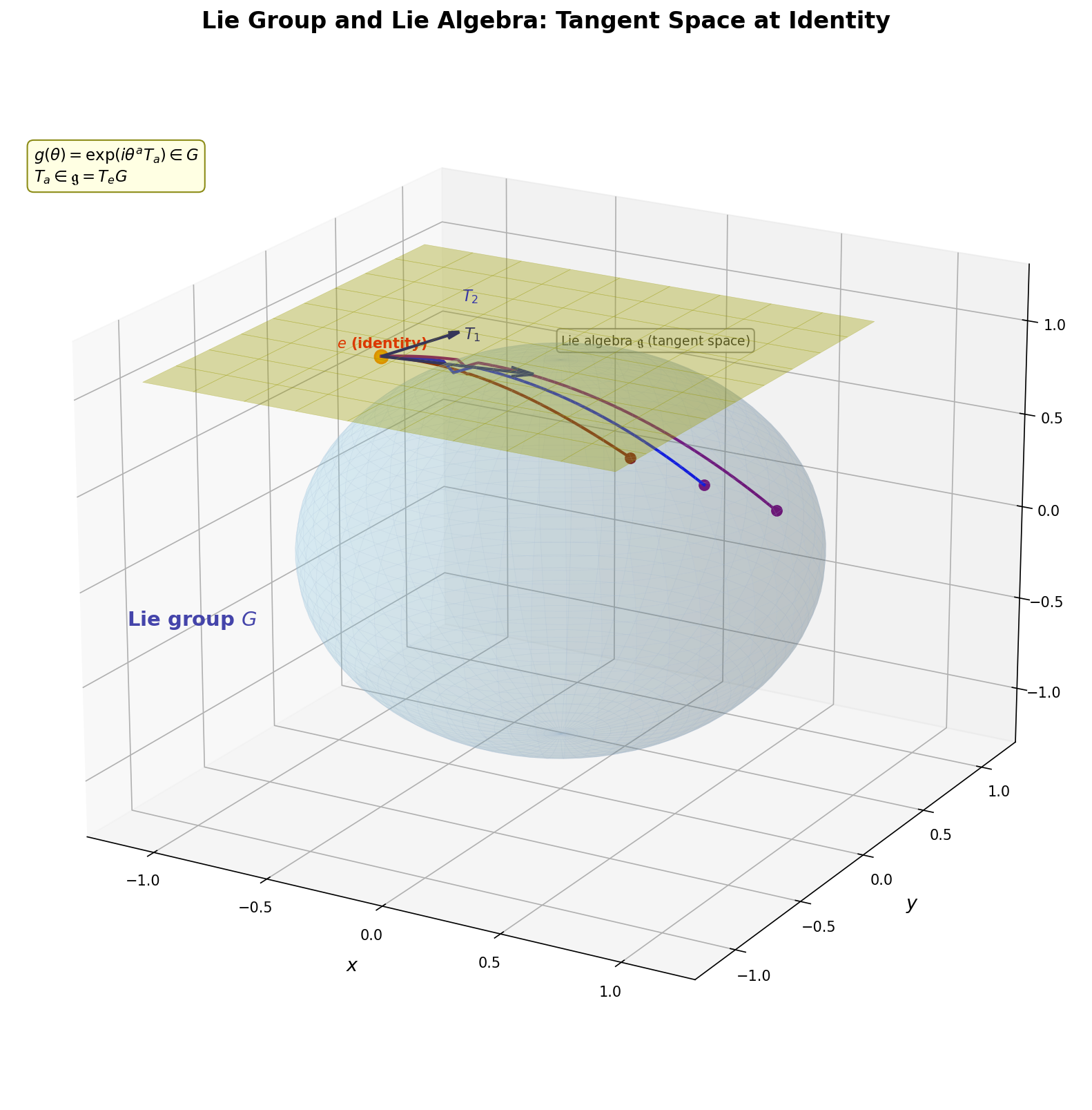
Fig. D.5: Relationship between Lie group and Lie algebra. Figure D_4: A Lie group has a surface-like structure, and the tangent space at the identity \(e\) corresponds to the Lie algebra. Generators are "directions of displacement" (tangent vectors) at the identity, and finite transformations can be recovered via the exponential map (\(e^{i\theta^a T_a}\)).
Infinitesimal Transformations and the Definition of Generators
Let's expand the \(SO(2)\) rotation matrix \(R(\theta)\) for very small \(\theta\):
When \(\theta \ll 1\), \(\cos\theta \approx 1 - \theta^2/2 \approx 1\), \(\sin\theta \approx \theta\), so:
Organizing:
This \(J\) is the generator of \(SO(2)\). A matrix that specifies the "direction of displacement" from the identity.
⚪ Mei: Can you recover the finite rotation \(R(\theta)\) from the generator \(J\)?
🟡 Lina: Yes. Using the exponential function:
Let's verify this. The matrix exponential is defined by its Taylor expansion:
Computing \(J^2\):
Therefore \(J^3 = J^2 \cdot J = -J\), \(J^4 = J^2 \cdot J^2 = I\), ... This follows the same pattern as \(i^2 = -1\)!
🔵 Kai: Oh, repeatedly multiplying by \(J\) cycles through \(I, J, -I, -J, I, \ldots\) It has the same structure as the imaginary unit.
🟡 Lina: Right. Organizing the expansion:
Indeed, \(R(\theta)\) is recovered.
✅ Comprehension Check: Write the relationship between the generator \(J\) and the finite transformation \(R(\theta)\) as an equation.
Answer
\(R(\theta) = e^{\theta J}\). Finite transformations can be recovered as the exponential of the generator. The matrix exponential is defined by the Taylor expansion \(e^{\theta J} = I + \theta J + (\theta J)^2/2! + \cdots\).
The General Lie Group Case
In general, expanding a Lie group element near the identity:
Here the superscript \(a\) on \(\epsilon^a\) is not a power but a label for "the \(a\)-th parameter" (numbered as \(\epsilon^1, \epsilon^2, \ldots\)). The \(T_a\) (\(a = 1, 2, \ldots, n\)) are the generators. \(n\) is the number of group parameters (the dimension of the group). \(i\epsilon^a T_a\) is shorthand for \(\sum_{a=1}^n i\epsilon^a T_a\). In the same spirit as Einstein's summation convention learned in Appendix C (when the same index appears up and down, sum over it), repeated indices are summed.
::: {.callout-warning}
Convention for Internal Group Indices
For indices of the group's internal space (\(a, b, c\), etc.), the metric is \(\delta_{ab}\) (the identity matrix), so there is no physical distinction between upper and lower indices. Therefore, depending on the literature, one may write \(f_{abc}\) with all lower indices, or mix upper and lower as in \(\epsilon^a T_a\). In this chapter, we adopt the relaxed convention "whenever repeated indices appear (regardless of position), sum over them." This differs from the convention for spacetime indices (\(\mu, \nu\), etc.) where the Minkowski metric \(\eta_{\mu\nu}\) is used to strictly distinguish upper and lower. If in doubt, explicitly writing \(\sum\) will cause no problems. :::
🔵 Kai: Wait, why is there an \(i\) in front?
🟡 Lina: Putting \(i\) in front is a physics convention to make the generators Hermitian. Let's verify why \(i\) makes them Hermitian: for \(U \approx I + i\epsilon^a T_a\) to be unitary (\(U^\dagger U = I\)), we need the product with \(U^\dagger = I - i\epsilon^a T_a^\dagger\) to be \(I\). To first order, \(U^\dagger U \approx I + i\epsilon^a(T_a - T_a^\dagger) = I\), so \(T_a = T_a^\dagger\) (Hermitian) is required.
🔵 Kai: What's good about being Hermitian?
🟡 Lina: A Hermitian matrix is one satisfying \(T_a^\dagger = T_a\) (taking the transpose and complex conjugate gives back the original). The eigenvalues of Hermitian matrices are always real.
🔵 Kai: What are eigenvalues again? Having something about the matrix be real is good because...?
🟡 Lina: An eigenvalue is a scalar \(\lambda\) satisfying \(A\mathbf{v} = \lambda\mathbf{v}\) for a matrix \(A\) (\(\mathbf{v} \neq \mathbf{0}\) is called the eigenvector). When you apply a matrix to a vector, generally both its direction and magnitude change. But for special vectors \(\mathbf{v}\), the direction doesn't change and only the magnitude gets multiplied by \(\lambda\)—that multiplier \(\lambda\) is the eigenvalue. For example, applying the \(2 \times 2\) matrix \(\begin{pmatrix}3&0\\0&1\end{pmatrix}\) to the vector \(\begin{pmatrix}1\\0\end{pmatrix}\) gives \(\begin{pmatrix}3\\0\end{pmatrix}\). The direction is the same and the magnitude is tripled—so the eigenvalue is 3. In quantum mechanics, the values obtained from measuring physical quantities (energy, spin, etc.) correspond to the eigenvalues of the corresponding operator. So eigenvalues being real guarantees that "measurement results are real numbers."
🔵 Kai: I see, so attaching \(i\) makes the generators Hermitian, and their eigenvalues are real—meaning they become values that come out of measurements.
🟡 Lina: Right. In the earlier \(SO(2)\) example, we wrote \(R(\theta) \approx I + \theta J\) without \(i\). That's the mathematics convention. To match the physics convention, define \(T = -iJ\) and write \(R(\theta) = e^{i\theta T}\) (\(iT = J\) so \(e^{i\theta T} = e^{\theta J}\), the same thing). That \(T\) is Hermitian can also be verified: \(J\) is real and antisymmetric (\(J^T = -J\)), so \(T^\dagger = (-iJ)^\dagger = (-i)^* J^\dagger = i J^T = i(-J) = -iJ = T\) ✓ (using \((-i)^* = i\), \(J^\dagger = J^T\) since \(J\) is real, and \(J^T = -J\) (antisymmetric)).
Hereafter we unify with the physics convention (\(i\) included). That is, we write a general Lie group element as \(U = e^{i\theta^a T_a}\), and infinitesimally as \(U \approx I + i\epsilon^a T_a\). In the earlier \(SO(2)\) example, \(R(\theta) = e^{\theta J} = e^{i\theta T}\) (\(T = -iJ\)) rewritten corresponds to the physics convention.
Finite transformations via the exponential:
🔵 Kai: Wait, isn't \(\theta^a\) the \(a\)-th power of \(\theta\)? It's written as a superscript so it looks like a power.
🟡 Lina: It is confusing. Here \(\theta^a\) means "the \(a\)-th parameter"—the superscript index is just a label, not a power. And \(\theta^a T_a = \sum_{a=1}^n \theta^a T_a\) follows the convention that when the same index \(a\) appears as a superscript (\(\theta^a\)) and subscript (\(T_a\)), you sum—the same Einstein summation convention from Appendix C, applied here to internal group indices. It's separate from spacetime indices \(\mu, \nu\), but the convention "repeated indices are summed" is shared. Until you get used to it, feel free to write \(\sum\) explicitly.
⚪ Mei: So the superscript \(a\) on \(\theta^a\) is a label, not a power, and when the same index appears up and down, you sum—the same convention as Appendix C.
✅ Comprehension Check: What is the physical reason for putting the imaginary unit \(i\) in front of the generators \(T_a\) when expanding a Lie group element near the identity?
Answer
To make the generators Hermitian (\(T_a^\dagger = T_a\)). Hermitian matrices have real eigenvalues, making it easier to identify generators with physical observables (like angular momentum).
Commutation Relations and Structure Constants
🟡 Lina: Here's the heart of the matter. The commutation relations between generators define the Lie algebra.
The index \(c\) on the right side is summed over (\(if_{abc}T_c = i\sum_c f_{abc}T_c\), by the internal index summation convention described earlier). The \(f_{abc}\) are the structure constants—numerical values that determine the "shape" of the group.
🔵 Kai: Why are commutation relations important?
🟡 Lina: The commutator measures whether the results of two operations \(A\) and \(B\) differ when done as "\(A\) then \(B\)" versus "\(B\) then \(A\)."
- \([A, B] = 0\): swapping the order gives the same result (commutative)
- \([A, B] \neq 0\): the order matters (non-commutative)
\(U(1)\) is commutative (addition of angles doesn't depend on order). \(SU(2)\) and \(SU(3)\) are non-commutative.
⚪ Mei: So if the commutator isn't zero, it's non-commutative, and the "amount of discrepancy" is quantified as the structure constants \(f_{abc}\).
🔵 Kai: But the commutation relation is "the discrepancy when swapping the order of two generators," right? It seems like too little information to determine the whole group picture, doesn't it?
🟡 Lina: Good intuition. But it's actually sufficient. Here's why: any element of the group can be written as \(e^{i\theta^a T_a}\). When computing the product of two elements \(e^{i\theta^a T_a} e^{i\phi^b T_b}\), expanding the exponentials produces products like \(T_a T_b\). Since \(T_a T_b = T_b T_a + [T_a, T_b]\), if you know the commutation relations, you can organize all products. In other words, the commutation relations completely determine the "multiplication rules" for generators, and that contains the information of the entire group.
✅ Comprehension Check: When the commutation relation \([T_a, T_b] = 0\) holds, what property do the two operations have?
Answer
The result is the same regardless of the order (commutative). Whether you do \(T_a\) first then \(T_b\), or the reverse order, the result is identical.
Concrete Computation: The \(SU(2)\) Lie Algebra
🟡 Lina: Let's concretely compute the generators of \(SU(2)\). There are 3 generators: \(T_i = \sigma_i / 2\) (\(\sigma_i\) are the Pauli matrices).
Let's compute \([T_1, T_2]\). Since \(T_i = \sigma_i/2\):
Computing \(\sigma_1 \sigma_2\):
Computing \(\sigma_2 \sigma_1\):
Therefore:
🔵 Kai: Oh, \(iT_3\) comes out cleanly!
🟡 Lina: Performing similar calculations for other combinations, in general:
Here \(\varepsilon_{ijk}\) is the Levi-Civita symbol (\(\varepsilon_{123} = 1\), \(+1\) for even permutations, \(-1\) for odd permutations, \(0\) if any two indices are the same). An even/odd permutation means: starting from \(123\) as reference, if you reach the desired arrangement by repeating transpositions (swapping any two indices), the permutation is even if the number of swaps is even, odd if odd. For example, \(231\) is reached from \(123 \to 213\) (swap 1 and 2) \(\to 231\) (swap 1 and 3), requiring 2 swaps, so it's an even permutation (\(\varepsilon_{231} = +1\)). \(132\) is reached from \(123 \to 132\) (swap 2 and 3), requiring 1 swap, so it's an odd permutation (\(\varepsilon_{132} = -1\)).
🟡 Lina: So the structure constants of \(SU(2)\) are \(f_{ijk} = \varepsilon_{ijk}\). And this has exactly the same form as the angular momentum commutation relations. If you've learned the spin commutation relations \([J_i, J_j] = i\hbar\varepsilon_{ijk}J_k\) in quantum mechanics (Quantum Mechanics Quantum Mechanics Ch. 15), you already knew the \(SU(2)\) Lie algebra (in units where \(\hbar = 1\)). By the way, the cyclic structure \([T_1, T_2] = iT_3\), \([T_2, T_3] = iT_1\), \([T_3, T_1] = iT_2\) follows the same pattern as the cross product \(\hat{x} \times \hat{y} = \hat{z}\).
⚪ Mei: I see, so in the general definition \([T_a, T_b] = if_{abc}T_c\), the \(f_{abc}\) concretely becomes \(\varepsilon_{ijk}\) for \(SU(2)\). Since it has the same cyclic structure as the cross product, if you remember \([T_1, T_2] = iT_3\), the rest can be obtained just by cycling the indices.
🟡 Lina: Exactly. This is the Lie algebra of \(SO(3)\) / \(SU(2)\). The angular momentum operators \(J_i\) in quantum mechanics (with \(J_i = T_i\) in units \(\hbar = 1\)) satisfy exactly the same commutation relations. Written out explicitly:
✅ Comprehension Check: What are the structure constants \(f_{ijk}\) of \(SU(2)\) equal to?
Answer
The Levi-Civita symbol \(\varepsilon_{ijk}\). \(\varepsilon_{123} = 1\), \(+1\) for even permutations, \(-1\) for odd permutations, and \(0\) when any two indices are the same.
📝 Exercises:
- Computing Pauli matrix commutation relations → Problem B-6. Commutation Relation of Pauli Matrices \([\sigma_1, \sigma_2]\), Problem B-7. Commutation Relations of Pauli Matrices (All Pairs), antisymmetry of commutators and Jacobi identity → Problem B-8. Antisymmetry of the Commutator, Problem M-2. Jacobi Identity (Verification with Pauli Matrices)
Properties of Structure Constants
The structure constants \(f_{abc}\) have important properties:
Antisymmetry: From the definition of the commutator \([T_a, T_b] = -[T_b, T_a]\),
That is, swapping the first two indices changes the sign.
Jacobi identity: For any three generators,
This can also be written in terms of structure constants (the indices get complex, so we just state the result):
(Sum over index \(e\). \(a, b, c, d\) are free indices.) This equation won't appear directly in this chapter, but the Jacobi identity is a consistency condition for the Lie algebra to be well-defined mathematically, and it also plays an important role in ensuring that gauge theories are physically consistent (for example, conservation of probability).
✅ Comprehension Check: What is the antisymmetry of the structure constants \(f_{abc}\)?
Answer
Swapping the first two indices changes the sign: \(f_{abc} = -f_{bac}\). This follows directly from the definition of the commutator \([T_a, T_b] = -[T_b, T_a]\).
The Virasoro Algebra (Preview for Chapter 16)
🟡 Lina: Let me also introduce, as a preview, a Lie algebra that appears in conformal field theory in string theory. For now, just getting a feel for it is enough.
The generators \(L_n\) (\(n\) is an integer) describing the symmetry (conformal symmetry) on the string worldsheet are infinite in number. Their commutation relations are:
Here \(\delta_{m+n,0}\) is the Kronecker delta (1 when \(m + n = 0\), 0 otherwise). The first term \((m-n)L_{m+n}\) has a structure similar to \(SU(2)\)'s \([T_i, T_j] = i\varepsilon_{ijk}T_k\) in that "the commutator of two generators is a linear combination of other generators." However, the second term is new. \(c\) is a constant called the central charge, a feature absent in finite-dimensional Lie algebras (like \(SU(2)\)). This term is what restricts the spacetime dimension of string theory to \(D = 26\) (bosonic string) or \(D = 10\) (superstring). Details are covered in Ch. 14, Ch. 16.
🔵 Kai: Infinite generators—that's a completely different scale from \(SU(2)\)'s three...
🟡 Lina: Yes. That's precisely why string theory has such rich structure. For now, just knowing "this exists" is enough.
✅ Comprehension Check: What are the \(f_{abc}\) appearing in the commutation relation \([T_a, T_b] = if_{abc}T_c\) of generators \(T_a\) that define a Lie algebra called?
Answer
Structure constants. Numerical values that determine the "shape" of the group.
✅ Comprehension Check: The Lie algebra commutation relations of \(SU(2)\) are the same as the commutation relations of which physical quantity in quantum mechanics?
Answer
Angular momentum (spin) commutation relations. \([J_i, J_j] = i\varepsilon_{ijk}J_k\).
D.5 Representations — "Viewing" a Group Through Matrices
What Is a Representation?
🟡 Lina: "Representing" the abstract elements of a group as concrete matrices. The same group can be represented by matrices of different sizes.
🔵 Kai: The same group but different matrix sizes?
🟡 Lina: Let me give an analogy. The abstract operation of "rotation" can rotate a 2D picture or a 3D object. The same "rotation" is represented by a \(2 \times 2\) matrix in 2D and a \(3 \times 3\) matrix in 3D. Even though the matrix sizes differ, the "structure" of rotation (commutation relations, etc.) remains the same.
Mathematically: a representation of a group \(G\) is a mapping that assigns a matrix \(D(g)\) to each element \(g\) of \(G\), preserving the group product:
The matrix size \(n\) is called the dimension of the representation.
✅ Comprehension Check: In a group representation, what does it mean to preserve the group product? Write it as an equation.
Answer
\(D(g_1) D(g_2) = D(g_1 \cdot g_2)\). The matrix corresponding to the product of group elements equals the product of the respective matrices.
Representations of \(SU(2)\) and Spin
For each spin quantum number \(j = 0, 1/2, 1, 3/2, 2, \ldots\), \(SU(2)\) has exactly one \((2j+1)\)-dimensional representation.
%%{init: {"theme": "default", "themeCSS": ".edgePath .path, .flowchart-link { stroke-width: 2px !important; }"}}%%
flowchart TD
    SU2["SU(2) group"] --> j0["j = 0<br/>1×1 matrices<br/>scalar particles"]
    SU2 --> j12["j = 1/2<br/>2×2 matrices<br/>electrons, quarks"]
    SU2 --> j1["j = 1<br/>3×3 matrices<br/>W bosons"]
    SU2 --> j32["j = 3/2<br/>4×4 matrices<br/>gravitino"]
    SU2 --> jdots["..."]
    style SU2 fill:#fef,stroke:#636
    style j12 fill:#ffd,stroke:#aa0
Fig. D.6: Spin representations of the SU(2) group and particles
Table D.3: Representations of SU(2) and spin quantum numbers
| Representation | Dimension \((2j+1)\) | Physical meaning |
|---|---|---|
| \(j = 0\) (trivial representation) | 1 | Scalar (spin 0) |
| \(j = 1/2\) (fundamental representation) | 2 | Spin \(1/2\) (electrons, quarks) |
| \(j = 1\) (adjoint representation, defined below) | 3 | Spin \(1\) (\(W\) bosons) |
| \(j = 3/2\) | 4 | Spin \(3/2\) (gravitino) |
The dimension of the adjoint representation of \(SU(2)\) equals the number of generators (= 3). Since \(2j+1 = 3\) gives \(j = 1\), the adjoint representation coincides with the spin-1 representation.
In the fundamental representation (\(j = 1/2\)), the generators are \(T_i = \sigma_i/2\) (\(2 \times 2\) matrices).
In the adjoint representation (\(j = 1\)), the generators are \(3 \times 3\) matrices whose components are the structure constants themselves:
Why is this definition natural? The commutation relation \([T_a, T_b] = if_{abc}T_c\) can be read as "\(T_a\) acts on \(T_b\) and rotates it into the \(T_c\) direction." In other words, the generators themselves act as matrices that "rotate" other generators—and the matrix components are precisely the structure constants \(f_{abc}\).
🔵 Kai: Huh, the structure constants directly become matrix entries. That's kind of self-referential and interesting.
🟡 Lina: The dimension of the adjoint representation equals the number of generators (\(SU(2)\): 3, \(SU(3)\): 8). This is the mathematical basis for "gauge fields belong to the adjoint representation" → "number of mediator particles = number of generators."
For \(SU(2)\), \((T_i)_{jk} = -i\varepsilon_{ijk}\). That is, the \((j, k)\) entry of matrix \(T_i\) is given by \(-i\varepsilon_{ijk}\). For example, the \((2,3)\) entry of \(T_1\) is obtained by substituting \(i=1, j=2, k=3\): \((T_1)_{23} = -i\varepsilon_{123} = -i\) (\(\varepsilon_{123} = +1\) is the fundamental ordering). The \((3,2)\) entry is \((T_1)_{32} = -i\varepsilon_{132} = +i\) (\(132\) is obtained by swapping the last two elements (2 and 3) of \(123\), one swap = odd permutation, so \(\varepsilon_{132} = -1\)). What about diagonal entries? For example, \((T_1)_{11} = -i\varepsilon_{111}\). Since \(\varepsilon_{ijk}\) is 0 whenever two or more indices are the same, \((T_1)_{11} = 0\). Similarly \((T_1)_{12} = -i\varepsilon_{112} = 0\), \((T_1)_{13} = -i\varepsilon_{113} = 0\). So the entire first row and first column of \(T_1\) are zero. Writing out all components similarly:
That these satisfy \([T_i, T_j] = i\varepsilon_{ijk}T_k\) can be confirmed by direct calculation.
Particle Classification in the Standard Model
In the Standard Model of Ch. 9, each particle belongs to a specific representation of the gauge group:
- Left-handed quarks: fundamental representation of \(SU(3)\) (3-dimensional) and fundamental representation of \(SU(2)\) (2-dimensional)
- Right-handed electrons: trivial representation of \(SU(2)\) (1-dimensional, meaning they don't feel the weak force)
- Gluons: adjoint representation of \(SU(3)\) (8-dimensional)
🔵 Kai: Huh, left-handed quarks are 3-dimensional in \(SU(3)\), 2-dimensional in \(SU(2)\)... so for each particle, "which representation it belongs to" is determined.
🟡 Lina: Yes. And conversely, symmetry classifies particles. Specifying the symmetry constrains what kinds of particles can exist. This is why group theory is so powerful in physics.
⚪ Mei: So a particle's properties are organized by the label "which representation of which group it belongs to."
✅ Comprehension Check: In the Standard Model, which representation of \(SU(3)\) do gluons belong to, and what is its dimension?
Answer
They belong to the adjoint representation, with dimension 8. This is why 8 types of gluons exist.
📝 Exercises:
- Eigenvalues and eigenvectors of spin \(1/2\) → Problem B-9. Eigenvalues and Eigenvectors of Spin 1/2
✅ Comprehension Check: What is a "representation" of a group?
Answer
Realizing the abstract elements of a group as concrete matrices. The same group can be represented by matrices of different sizes.
✅ Comprehension Check: The fundamental representation (\(2 \times 2\) matrices) of \(SU(2)\) corresponds physically to particles of what spin?
Answer
Spin \(1/2\) particles (electrons, quarks, etc.).
D.6 Symmetry and Conservation Laws — Deriving Noether's Theorem
Statement of the Theorem
🟡 Lina: Every continuous symmetry has a corresponding conserved quantity. This is Noether's theorem. We already touched on it in Quantum Mechanics Quantum Mechanics Ch. 26 and Quantum Field Theory Quantum Field Theory Ch. 3, but here we'll carefully derive the field theory version.
Derivation
Consider the action of a field \(\phi(x)\). The action is a quantity representing the "cost" of a field's motion. You may have learned in high school physics that "light takes the shortest path" (Fermat's principle)—in the same spirit, fields in nature choose "the configuration that minimizes (more precisely, makes stationary) the action"—this is the principle of least action. Newton's equations of motion can actually be derived from this principle (Quantum Field Theory Quantum Field Theory Ch. 3). The action is the Lagrangian density \(\mathcal{L}\) integrated over all spacetime:
Here \(\mathcal{L}\) is a function of the field \(\phi\) and its derivatives \(\partial_\mu\phi\) (\(\mu = 0, 1, 2, 3\), comprising the time derivative \(\partial_0\phi = \partial\phi/\partial t\) and spatial derivatives \(\partial_i\phi\), totaling 4 components). \(d^4x = dt\,dx\,dy\,dz\) is the 4-dimensional spacetime volume element. The equation derived from minimizing the action is the Euler-Lagrange equation (equation of motion):
The second term is summed over \(\mu = 0, 1, 2, 3\) (the convention that when the same index \(\mu\) appears repeatedly, you sum). Expanded: \(\partial_0\frac{\partial\mathcal{L}}{\partial(\partial_0\phi)} + \partial_1\frac{\partial\mathcal{L}}{\partial(\partial_1\phi)} + \partial_2\frac{\partial\mathcal{L}}{\partial(\partial_2\phi)} + \partial_3\frac{\partial\mathcal{L}}{\partial(\partial_3\phi)}\), a sum of 4 terms. For example, the \(\mu = 2\) term means "differentiate \(\mathcal{L}\) with respect to \(\partial_2\phi\), then differentiate that result with respect to \(x^2\)."
🔵 Kai: Wait, \(\frac{\partial\mathcal{L}}{\partial(\partial_\mu\phi)}\) means "differentiating by a derivative"? What's being treated as a variable?
🟡 Lina: Good question. Think of \(\mathcal{L}\) as a function that takes \(\phi\) and \(\partial_\mu\phi\) as two "independent variables." When you take the partial derivative \(f(x, y)\) with respect to \(x\), you treat \(y\) as a constant, right? Similarly, \(\partial\mathcal{L}/\partial\phi\) is "the rate of change when only \(\phi\) varies while \(\partial_\mu\phi\) is held fixed," and \(\partial\mathcal{L}/\partial(\partial_\mu\phi)\) is "the rate of change when only \(\partial_\mu\phi\) varies while \(\phi\) is held fixed." The notation looks strange, but what it's doing is ordinary partial differentiation.
Intuitively, the first term \(\frac{\partial\mathcal{L}}{\partial\phi}\) represents "how the value of field \(\phi\) itself affects the Lagrangian," while the second term represents "how the rate of change (derivative) of the field affects it"—the balance between both determines the equation of motion. In terms of Newton's \(F = ma\), this corresponds to the balance between force (derivative of potential) and acceleration (second derivative of position).
🔵 Kai: So it's like a "field version" of Newton's equation of motion. But honestly I don't quite see yet why it takes this form.
🟡 Lina: Thanks for being honest. Simply put, "minimizing the action \(S\)" means "when \(S\) is varied slightly, the change is zero." It's the same idea as \(f'(x) = 0\) at the minimum of \(f(x)\). In fact, for a 1D particle, applying the Euler-Lagrange equation \(\frac{\partial L}{\partial x} - \frac{d}{dt}\frac{\partial L}{\partial \dot{x}} = 0\) to \(L = \frac{1}{2}m\dot{x}^2 - V(x)\) gives \(\frac{\partial L}{\partial x} = -V'(x)\) and \(\frac{\partial L}{\partial \dot{x}} = m\dot{x}\), so \(-V'(x) - m\ddot{x} = 0\), i.e., \(m\ddot{x} = -V'(x)\)—Newton's \(F = ma\) comes right out. The field theory version is an extension: instead of particle position \(x(t)\), we have field \(\phi(x)\); instead of velocity \(\dot{x}\), we have field derivative \(\partial_\mu\phi\). Here's a correspondence table:
| Particle mechanics | Field theory |
|---|---|
| Position \(x(t)\) | Field \(\phi(x)\) |
| Velocity \(\dot{x}\) | Field derivative \(\partial_\mu\phi\) |
| Time \(t\) | Spacetime coordinates \(x^\mu\) |
| \(\frac{\partial L}{\partial x} - \frac{d}{dt}\frac{\partial L}{\partial\dot{x}} = 0\) | \(\frac{\partial\mathcal{L}}{\partial\phi} - \partial_\mu\frac{\partial\mathcal{L}}{\partial(\partial_\mu\phi)} = 0\) |
⚪ Mei: The correspondence between particle mechanics and field theory lines up beautifully. The structure is the same, just with more variables.
🟡 Lina: The detailed derivation is done carefully in Quantum Field Theory Quantum Field Theory Ch. 3, so here let's accept it as "the equation of motion that comes from minimizing the action" and move forward.
We're about to derive Noether's theorem, and we'll only need three things: the Euler-Lagrange equation above, the product rule \((fg)' = f'g + fg'\) learned in high school, and the total differential of a multivariable function (\(\Delta f \approx \frac{\partial f}{\partial x}\Delta x + \frac{\partial f}{\partial y}\Delta y\)). I'll explain the total differential shortly, so don't worry. If you accept the Euler-Lagrange equation as "for fields satisfying the equations of motion, a certain quantity is zero," you should be able to follow the rest.
Under a continuous transformation \(\phi(x) \to \phi(x) + \delta\phi(x)\), the change in the Lagrangian density is:
This has the same structure as the total differential of a multivariable function. For one variable, you learned in high school that changing \(f(x)\) from \(x\) to \(x + \Delta x\) gives \(\Delta f \approx f'(x)\Delta x\). For two variables, it's the extension: the small change in \(f(x, y)\) is \(\Delta f \approx \frac{\partial f}{\partial x}\Delta x + \frac{\partial f}{\partial y}\Delta y\)—you just add up the contributions from each variable's change. In the same way, this represents the change in \(\mathcal{L}(\phi, \partial_\mu\phi)\) when its two "variables" \(\phi\) and \(\partial_\mu\phi\) change by \(\delta\phi\) and \(\delta(\partial_\mu\phi)\) respectively (the second term is summed over \(\mu\)).
🔵 Kai: I see, so you just add up the changes from each variable. The name "total differential" sounds grand but what it does is simple.
🟡 Lina: \(\delta\) and \(\partial_\mu\) can be commuted. \(\delta\) is the operation "slightly changing the shape of the field" and \(\partial_\mu\) is "looking at the slope at a point"—they don't interfere with each other. Let's verify concretely: suppose \(\phi\) is changed to \(\phi + \epsilon\, \eta(x)\) (\(\eta(x)\) is the "shape" of the variation). Then \(\delta\phi = \epsilon\,\eta\), and \(\partial_\mu(\delta\phi) = \epsilon\,\partial_\mu\eta\). Meanwhile, \(\delta(\partial_\mu\phi) = \partial_\mu(\phi + \epsilon\,\eta) - \partial_\mu\phi = \epsilon\,\partial_\mu\eta\). They indeed agree. So \(\delta(\partial_\mu\phi) = \partial_\mu(\delta\phi)\). Substituting:
From here, the goal is to separate \(\delta\mathcal{L}\) into "the equations-of-motion part" and "a total derivative part." For this, we rewrite the second term using the product rule:
Using this:
Substituting back:
⚪ Mei: The first term has exactly the form of the Euler-Lagrange equation.
🟡 Lina: Exactly. The \([\cdots]\) in the first term is the Euler-Lagrange equation (equation of motion) itself. For fields satisfying the equations of motion (on-shell), this is zero:
Therefore, when the equation of motion holds:
Here, the transformation being a symmetry means the action \(S\) is invariant. The simplest case is \(\delta\mathcal{L} = 0\) (the Lagrangian density itself is invariant), giving:
where the Noether current \(j^\mu\) is:
When the field has multiple components (for example, a complex field \(\phi\) and \(\phi^*\)), contributions from each component are added: \(j^\mu = \sum_i \frac{\partial\mathcal{L}}{\partial(\partial_\mu\phi_i)}\,\delta\phi_i\). We'll actually use this in Example 2.
More generally, even if \(\delta\mathcal{L}\) isn't zero but takes the form of a total derivative \(\delta\mathcal{L} = \partial_\mu K^\mu\), the action is still invariant (under conditions where boundary terms vanish), and the conserved current is modified to \(j^\mu - K^\mu\). The spatial translation example (below) falls into this more general case, but the essential structure is the same.
\(\partial_\mu j^\mu = 0\) is a conservation law (continuity equation). The corresponding conserved charge is:
Why \(Q\) is conserved: integrating \(\partial_\mu j^\mu = \partial_0 j^0 + \partial_i j^i = 0\) over all space gives \(\frac{dQ}{dt} = -\int d^3x\, \partial_i j^i\). By Gauss's theorem, the right side becomes a surface integral at the boundary (at infinity), which vanishes when fields go to zero at infinity. Thus \(\frac{dQ}{dt} = 0\) (\(Q\) doesn't change with time).
🔵 Kai: Wait. Using the product rule in the middle to split terms was to create the Euler-Lagrange equation form.
🟡 Lina: Exactly. For fields satisfying the equation of motion, the first term vanishes, so the remainder takes the form of a total derivative. That's the conservation law.
🔵 Kai: Amazing. Just assuming symmetry (\(\delta\mathcal{L} = 0\)) automatically produces a conserved quantity.
🟡 Lina: Yes. That's the power of Noether's theorem. Let's look at concrete examples.
Example 1: Spatial Translation → Momentum Conservation
::: {.callout-tip}
Reading Hint
This example involves somewhat heavy index manipulations. If you get stuck partway through, try reading "Example 2: \(U(1)\) phase transformation → charge conservation" first, then come back—the structure of Noether's theorem will become clearer. :::
This example is slightly more complex than the derivation above, falling into the case where \(\delta\mathcal{L} \neq 0\) but equals a total derivative. "\(\delta\mathcal{L}\) being a total derivative" means it isn't zero but can be written as \(\delta\mathcal{L} = \partial_\mu(\text{something})\)—in this case, the action integral is still invariant under boundary conditions.
Transformation: \(\phi(x) \to \phi(x + \epsilon) \approx \phi(x) + \epsilon^\nu \partial_\nu\phi\)
So \(\delta\phi = \epsilon^\nu \partial_\nu\phi\). For each direction \(\nu\), one Noether current is obtained. For a translation in the \(\nu\) direction:
Since \(\delta\phi = \epsilon^\nu\partial_\nu\phi\) for spatial translations, substituting into the Noether current formula \(j^\mu = \frac{\partial\mathcal{L}}{\partial(\partial_\mu\phi)}\delta\phi\) gives \(\frac{\partial\mathcal{L}}{\partial(\partial_\mu\phi)}\epsilon^\nu\partial_\nu\phi\).
However, under spatial translations, the Lagrangian density itself also changes—not to zero but as a total derivative. Why? \(\mathcal{L}\) is a function of \(\phi\) and \(\partial_\mu\phi\), but since \(\phi(x)\) itself depends on \(x\), \(\mathcal{L}\) is ultimately also a function of \(x\). Shifting space by \(\epsilon\) changes the value of \(\mathcal{L}\) by the amount the position shifts. Concretely, \(\mathcal{L}(x) \to \mathcal{L}(x + \epsilon) \approx \mathcal{L}(x) + \epsilon^\nu\partial_\nu\mathcal{L}(x)\). So \(\delta\mathcal{L} = \epsilon^\nu\partial_\nu\mathcal{L}\). Since \(\epsilon^\nu\) is a constant (an infinitesimal quantity independent of position), it can be taken outside \(\partial_\mu\). Here we want to rewrite \(\partial_\nu\mathcal{L}\) in the form \(\partial_\mu(\cdots)\). The reason we want to do this is that ultimately we want to "combine the Noether current \(j^\mu\) part and the \(\delta\mathcal{L}\) part inside the same \(\partial_\mu\), then subtract" to arrive at the form \(\partial_\mu(\cdots) = 0\) (a conservation law). For this, both need to be written as \(\partial_\mu(\cdots)\) with the same index \(\mu\). No physical content changes—it's just preparation for aligning indices.
For this we use the Kronecker delta \(\delta^\mu_\nu\). This is a symbol equal to 1 when \(\mu = \nu\) and 0 when \(\mu \neq \nu\). For example, \(\delta^0_0 = 1\), \(\delta^1_0 = 0\), \(\delta^2_2 = 1\), etc. Its most important property is "selecting an index": \(\sum_\mu \delta^\mu_\nu A_\mu = A_\nu\) (only the \(\mu = \nu\) term survives, the rest vanish as 0). Concretely, for \(\nu = 2\): \(\sum_\mu \delta^\mu_2 A_\mu = \delta^0_2 A_0 + \delta^1_2 A_1 + \delta^2_2 A_2 + \delta^3_2 A_3 = 0 + 0 + A_2 + 0 = A_2\).
Using this, we can rewrite \(\partial_\nu\mathcal{L} = \delta^\mu_\nu\partial_\mu\mathcal{L}\). Therefore \(\delta\mathcal{L} = \epsilon^\nu \delta^\mu_\nu\partial_\mu\mathcal{L} = \partial_\mu(\epsilon^\nu \delta^\mu_\nu \mathcal{L})\) (the last equality holds because \(\epsilon^\nu \delta^\mu_\nu\) is constant, so it can be placed inside \(\partial_\mu\)). This falls into the general case mentioned earlier: "if \(\delta\mathcal{L}\) is a total derivative \(\partial_\mu K^\mu\), the conserved current is modified to \(j^\mu - K^\mu\)." Since \(\delta\mathcal{L} = \epsilon^\nu\partial_\nu\mathcal{L} = \partial_\mu(\epsilon^\nu\delta^\mu_\nu\mathcal{L})\), we have \(K^\mu = \epsilon^\nu\delta^\mu_\nu\mathcal{L}\) (where \(\delta^\mu_\nu\) is the Kronecker delta: 1 when \(\mu = \nu\), 0 otherwise; it serves to select the index as in \(\sum_\mu \delta^\mu_\nu A_\mu = A_\nu\)). The modified conserved current is \(j^\mu - K^\mu\):
In the last equality, \(\epsilon^\nu\) was factored out as a common factor. Define the quantity in brackets as \(T^\mu{}_\nu\):
The conservation law for the conserved current \(\partial_\mu(j^\mu - K^\mu) = 0\) becomes \(\partial_\mu(\epsilon^\nu T^\mu{}_\nu) = \epsilon^\nu \partial_\mu T^\mu{}_\nu = 0\) (\(\epsilon^\nu\) is constant so it can be taken outside \(\partial_\mu\)). Since \(\epsilon^\nu\) is an arbitrary infinitesimal constant vector, for \(\epsilon^\nu \partial_\mu T^\mu{}_\nu = 0\) to hold for arbitrary \(\epsilon^\nu\), we must have \(\partial_\mu T^\mu{}_\nu = 0\) for each \(\nu\) (the argument: if \(\epsilon^\nu X_\nu = 0\) holds for arbitrary \(\epsilon^\nu\), then \(X_\nu = 0\)). That is, the canonical energy-momentum tensor \(T^\mu{}_\nu\) satisfies the conservation law:
Here \(T^\mu{}_\nu\) has an upper index \(\mu\) and a lower index \(\nu\), where \(\mu\) specifies the "direction of flow" and \(\nu\) specifies the "direction of translation" (\(\nu = 0\) is the time direction, \(\nu = 1, 2, 3\) are spatial directions). This quantity describes the "flow" of the field's energy and momentum (see Quantum Field Theory Quantum Field Theory Ch. 3 for details). The conserved charge is:
For \(\nu = 1, 2, 3\), \(P_\nu\) corresponds to momentum in each direction. For \(\nu = 0\), the conserved quantity corresponds to energy (the exact sign depends on the metric sign convention, but the essential correspondence is "time translation → energy conservation, spatial translation → momentum conservation"). Thus, momentum conservation is derived from spatial translation symmetry, and energy conservation from time translation symmetry.
🔵 Kai: Honestly, with all the indices flying around, I couldn't follow every step of the calculation. But the conclusion is "if physics doesn't change when you shift space → momentum is conserved," right?
🟡 Lina: Yes, that's the conclusion. Think of the intermediate index manipulations as practice from Appendix C. The important thing is that the "symmetry → conservation law" structure will be seen much more clearly in the next \(U(1)\) example, so it's fine to understand that one first and come back.
Example 2: \(U(1)\) Phase Transformation → Charge Conservation
Transformation on a complex scalar field \(\phi\): \(\phi \to e^{i\alpha}\phi \approx \phi + i\alpha\phi\) (\(\alpha \ll 1\))
So \(\delta\phi = i\alpha\phi\). The Noether current is:
A complex field \(\phi\) packages two real fields—the real part \(\phi_1\) and imaginary part \(\phi_2\) (\(\phi = \phi_1 + i\phi_2\)).
🔵 Kai: Wait, \(\phi^*\) is automatically determined once \(\phi\) is determined, right? Why can we treat it as an "independent variable"?
🟡 Lina: Good question. Actually, treating \(\phi\) and \(\phi^*\) independently is mathematically equivalent to treating \(\phi_1 = (\phi + \phi^*)/2\) and \(\phi_2 = (\phi - \phi^*)/(2i)\) independently. It's just a change of variables from \((\phi_1, \phi_2)\) to \((\phi, \phi^*)\). It's a technique that simplifies partial derivative calculations.
🔵 Kai: Ah, it's the same thing as treating real and imaginary parts separately, just done with \(\phi\) and \(\phi^*\).
🟡 Lina: Right. Let's continue. Since \(\delta\phi = i\alpha\phi\) and \(\delta\phi^* = -i\alpha\phi^*\), the Noether current adds contributions from both. Substituting into the general formula \(j^\mu = \frac{\partial\mathcal{L}}{\partial(\partial_\mu\phi_i)}\,\delta\phi_i\) gives \(\alpha\left[\frac{\partial\mathcal{L}}{\partial(\partial_\mu\phi)}\,(i\phi) + \frac{\partial\mathcal{L}}{\partial(\partial_\mu\phi^*)}\,(-i\phi^*)\right]\). The conservation law \(\partial_\mu j^\mu = 0\) still holds after dividing by the constant \(\alpha\), so we redefine the Noether current as the part without \(\alpha\):
For example, consider the free complex scalar field \(\mathcal{L} = (\partial_\mu\phi)^*(\partial^\mu\phi) - m^2\phi^*\phi\). Stating the conclusion first: \(\frac{\partial\mathcal{L}}{\partial(\partial_\mu\phi)} = \partial^\mu\phi^*\) (similarly \(\frac{\partial\mathcal{L}}{\partial(\partial_\mu\phi^*)} = \partial^\mu\phi\)). Intuitively, this is the operation of "reading off the partner multiplying \(\partial_\mu\phi\) in \(\mathcal{L}\)"—the same as differentiating \(f(x,y) = xy\) with respect to \(x\) leaving \(y\).
::: {.callout-tip}
For First-Time Readers
The following index manipulation details can be skipped on first reading—you may proceed to the paragraph starting "Substituting these into the Noether current formula." Just remembering the conclusions is sufficient: \(\frac{\partial\mathcal{L}}{\partial(\partial_\mu\phi)} = \partial^\mu\phi^*\), \(\frac{\partial\mathcal{L}}{\partial(\partial_\mu\phi^*)} = \partial^\mu\phi\). Substituting these into the Noether current formula gives the final result \(j^\mu = i(\phi\,\partial^\mu\phi^* - \phi^*\,\partial^\mu\phi)\). :::
Treating \(\phi\) and \(\phi^*\) as independent variables, the part of \(\mathcal{L}\) containing \(\partial_\mu\phi\) is \((\partial_\mu\phi)^*(\partial^\mu\phi)\). Here \(\partial^\mu\phi \equiv \eta^{\mu\nu}\partial_\nu\phi\) is the "derivative with raised index" learned in Appendix C, converting a lower index to upper using the Minkowski metric \(\eta^{\mu\nu}\).
Stating the conclusion first:
This is the operation of "reading off the coefficient multiplying \(\partial_\mu\phi\) in \(\mathcal{L}\)." Let's verify below.
First, practice with a simple case. If \(\mathcal{L}\) were simply \(\mathcal{L} = (\partial_0\phi^*)(\partial_0\phi)\), then \(\frac{\partial\mathcal{L}}{\partial(\partial_0\phi)} = \partial_0\phi^*\) is obvious (same as differentiating \(f(x) = ax\) with respect to \(x\) leaving \(a\)). For the general case, writing \((\partial_\mu\phi)^*(\partial^\mu\phi)\) with explicit indices: \(\sum_{\nu}(\partial_\nu\phi^*)(\eta^{\nu\rho}\partial_\rho\phi)\) (summing over \(\nu\) and \(\rho\)). We want to find \(\frac{\partial\mathcal{L}}{\partial(\partial_\mu\phi)}\). Note: \(\mu\) here is not a summed index but a fixed specific value (for example, if \(\mu = 2\), it means "differentiate with respect to \(\partial_2\phi\)"). We treat \(\partial_0\phi\), \(\partial_1\phi\), \(\partial_2\phi\), \(\partial_3\phi\) as 4 independent variables and differentiate with respect to one of them, \(\partial_\mu\phi\).
Think of it the same way as the simple case above.
::: {.callout-tip}
Note on Reading Indices
Here \(\mu\) is a fixed specific value (e.g., \(\mu = 2\)), not a summed index. "Differentiating with respect to \(\partial_\mu\phi\)" means "among the 4 independent variables \(\partial_0\phi, \partial_1\phi, \partial_2\phi, \partial_3\phi\), differentiating with respect to the \(\mu\)-th one." :::
In \(\sum_{\rho}\eta^{\nu\rho}\partial_\rho\phi\), the only term containing \(\partial_\mu\phi\) is the \(\rho = \mu\) term (namely \(\eta^{\nu\mu}\partial_\mu\phi\)). Other \(\rho \neq \mu\) terms don't contain \(\partial_\mu\phi\) and are treated as "constants," giving zero when differentiated. So only the coefficient \(\eta^{\nu\mu}\) from the \(\rho = \mu\) term remains. Summing over \(\nu\) gives \(\sum_{\nu}(\partial_\nu\phi^*)\eta^{\nu\mu}\). Since the Minkowski metric is symmetric (\(\eta^{\nu\mu} = \eta^{\mu\nu}\)), \(\sum_{\nu}(\partial_\nu\phi^*)\eta^{\nu\mu} = \sum_{\nu}\eta^{\mu\nu}\partial_\nu\phi^* \equiv \partial^\mu\phi^*\). Similarly \(\frac{\partial\mathcal{L}}{\partial(\partial_\mu\phi^*)} = \partial^\mu\phi\). Substituting these into the Noether current formula:
::: {.callout-note}
On Sign Conventions
Some references adopt \(j^\mu = i(\phi^*\,\partial^\mu\phi - \phi\,\partial^\mu\phi^*)\) (with the overall sign reversed). This is a difference in convention regarding which sign of \(\alpha\) is chosen in the definition of \(\delta\phi\), and corresponds to the definition of the sign of charge \(Q\). The physical conclusion (that charge is conserved) is the same regardless of convention. Here we adopt the form that follows directly from substituting into the Noether current formula. :::
The conserved charge \(Q = \int d^3x\, j^0\) is the electric charge. Charge conservation is a consequence of \(U(1)\) symmetry.
✅ Comprehension Check: What is the conserved quantity corresponding to the \(U(1)\) phase symmetry \(\phi \to e^{i\alpha}\phi\) via Noether's theorem?
Answer
Electric charge. From \(U(1)\) symmetry, Noether's theorem derives charge conservation.
Summary Table
Table D.4: Noether's theorem: correspondence between symmetries and conserved quantities
| Symmetry | Transformation | Conserved quantity |
|---|---|---|
| Time translation | \(t \to t + \epsilon\) | Energy |
| Spatial translation | \(\mathbf{x} \to \mathbf{x} + \boldsymbol{\epsilon}\) | Momentum |
| Rotation | \(\mathbf{x} \to R\mathbf{x}\) | Angular momentum |
| \(U(1)\) gauge | \(\psi \to e^{i\theta}\psi\) | Electric charge |
| \(SU(3)\) gauge | Color transformation of quarks | Color charge |
%%{init: {"theme": "default", "themeCSS": ".edgePath .path, .flowchart-link { stroke-width: 2px !important; }"}}%%
flowchart LR
    subgraph Symmetry
        T["Time translation"]
        X["Spatial translation"]
        R["Rotation"]
        U["U(1) gauge"]
    end
    subgraph Conserved_Quantity["Conserved quantity"]
        E["Energy"]
        P["Momentum"]
        L["Angular momentum"]
        Q["Charge"]
    end
    T -->|Noether| E
    X -->|Noether| P
    R -->|Noether| L
    U -->|Noether| Q
Fig. D.7: Noether's theorem: symmetries and conserved quantities
The more symmetries there are, the more conserved quantities. The more conserved quantities, the more the system's behavior is constrained. This is why symmetry is overwhelmingly important in physics.
✅ Comprehension Check: What does Noether's theorem state?
Answer
Every continuous symmetry has a corresponding conserved quantity (e.g., time translation symmetry → energy conservation).
✅ Comprehension Check: What is the conserved quantity corresponding to spatial translation symmetry?
Answer
Momentum.
D.7 Gauge Symmetry and Covariant Derivatives
From Global Symmetry to Local Symmetry
🟡 Lina: The \(U(1)\) symmetry \(\phi \to e^{i\alpha}\phi\) we saw in Section D.6 has \(\alpha\) as a constant (the same value everywhere in spacetime). This is called a global symmetry.
Now let's make a stronger demand: require that physics doesn't change even when \(\alpha\) can be chosen independently at each spacetime point, i.e., \(\alpha \to \alpha(x)\). This is a local symmetry, namely a gauge symmetry.
🔵 Kai: Why deliberately make such a strong demand?
🟡 Lina: Historically, it's an extension of general relativity's spirit that "physical laws should not depend on the choice of coordinate system." And remarkably, requiring local symmetry causes a field that mediates forces (gauge field) to automatically appear. Forces are born from symmetry.
Discovering the Problem: Ordinary Derivatives Are Not Gauge-Invariant
Consider the Lagrangian of a free complex scalar field (the same one used in Example 2 of Section D.6; \(\partial^\mu = \eta^{\mu\nu}\partial_\nu\) uses the index raising from Appendix C):
The first term \((\partial_\mu\phi)^*(\partial^\mu\phi)\) corresponds to the "kinetic energy" of the field, measuring how much the field varies across spacetime. The second term \(m^2\phi^*\phi\) is the "mass term" describing a particle of mass \(m\).
Here \((\partial_\mu\phi)^*(\partial^\mu\phi)\) is summed over \(\mu = 0, 1, 2, 3\) (Einstein summation convention). Since \(\partial^\mu\phi = \eta^{\mu\nu}\partial_\nu\phi\) raises the index (see Appendix C), expanding with the Minkowski metric \(\eta^{\mu\nu} = \text{diag}(-1,+1,+1,+1)\) gives \(-|\partial_0\phi|^2 + |\partial_1\phi|^2 + |\partial_2\phi|^2 + |\partial_3\phi|^2\). The minus sign in front of the time derivative is a consequence of the Minkowski metric sign convention, and is standard in relativistic field theory.
::: {.callout-note}
On Sign Conventions
This chapter uses the same sign convention as the General Relativity volume: \(\eta_{\mu\nu} = \text{diag}(-1,+1,+1,+1)\). The Quantum Field Theory volume uses the opposite convention \((+,-,-,-)\), so please be aware. Physical conclusions do not depend on the convention. :::
Under the global transformation \(\phi \to e^{i\alpha}\phi\) (\(\alpha\) = constant):
So \(\mathcal{L}\) is invariant. No problem.
However, under a local transformation \(\phi(x) \to e^{i\alpha(x)}\phi(x)\) (\(\alpha(x)\) depends on position):
An unwanted term \(i(\partial_\mu\alpha)\phi\) appears! \(\partial_\mu\phi\) cannot factor out just \(e^{i\alpha(x)}\) in front. In other words, the ordinary derivative \(\partial_\mu\) does not transform "nicely" under local gauge transformations.
⚪ Mei: If \(\alpha\) is constant then \(\partial_\mu\alpha = 0\) and there's no problem, but when it depends on position, the derivative produces an extra term.
The Solution: Introducing the Covariant Derivative
🟡 Lina: To solve this problem, we introduce a new field \(A_\mu(x)\) (the gauge field) and define the covariant derivative:
Here \(g\) is the coupling constant (a parameter determining the strength of the force).
Let's require that \(D_\mu\phi\) transforms the same way as \(\phi\) (i.e., \(D_\mu\phi \to e^{i\alpha(x)}D_\mu\phi\)). This will determine the transformation rule for \(A_\mu\).
Computing the transformation of \(D_\mu\phi\). Writing the covariant derivative after gauge transformation as \(D'_\mu = \partial_\mu - igA'_\mu\) (\(A_\mu\) changed to \(A'_\mu\)):
For this to equal \(e^{i\alpha}D_\mu\phi = e^{i\alpha}(\partial_\mu - igA_\mu)\phi\):
\(\partial_\mu\phi\) cancels on both sides. Dividing by \(\phi\):
Solving:
This is the gauge field transformation rule. It's the same form as the "gauge transformation \(A_\mu \to A_\mu + \partial_\mu\Lambda\)" learned in electromagnetism!
🔵 Kai: Oh, it cancels out perfectly! \(A_\mu\) transforms just right to cancel the unwanted term.
✅ Comprehension Check: What is the purpose of introducing the covariant derivative \(D_\mu = \partial_\mu - igA_\mu\)?
Answer
To make \(D_\mu\phi\) transform the same way as \(\phi\) under local gauge transformations (\(D_\mu\phi \to e^{i\alpha(x)}D_\mu\phi\)). It solves the problem that the ordinary derivative \(\partial_\mu\) produces an unwanted \(\partial_\mu\alpha\) term.
🔵 Kai: Wait, just by requiring local symmetry, the electromagnetic field appeared? But how do we know \(A_\mu\) is the electromagnetic potential? Isn't it just "a new field we introduced"?
🟡 Lina: Good question. The first clue is that \(A_\mu\)'s transformation rule \(A_\mu \to A_\mu + \frac{1}{g}\partial_\mu\alpha\) has the same form as the gauge transformation learned in electromagnetism (Ch. 2). Furthermore, deriving the equation of motion for \(A_\mu\) from the gauge-invariant Lagrangian written at the end of Section D.7 gives Maxwell's equations (derivation in Quantum Field Theory Quantum Field Theory Ch. 3). From these two facts, we identify \(A_\mu\) as the electromagnetic potential (the photon field). Requiring local \(U(1)\) symmetry → gauge field (photon) necessarily appears → electromagnetism is derived. This is the heart of the gauge principle.
🔵 Kai: So if we do the same thing with \(SU(2)\) or \(SU(3)\), the weak force and strong force come out?
🟡 Lina: Exactly right. Requiring local \(SU(2)\) symmetry produces the \(W\) and \(Z\) bosons, and \(SU(3)\) produces 8 gluons. The exact same logical structure.
⚪ Mei: To summarize: "ordinary derivatives break under local transformations → introduce gauge fields to compensate → those gauge fields turn out to be force mediator particles"—a three-step process. Once you decide the starting point (requiring local symmetry), everything else follows necessarily.
🟡 Lina: Right. The existence of forces is derived just from requiring symmetry—that's the power of the gauge principle.
🔵 Kai: But conversely, "why we require local symmetry" itself isn't explained, right? Is that something we can only verify experimentally?
🟡 Lina: Sharp. Indeed, "why nature chose local symmetry" is essentially an axiom at present. However, assuming local symmetry gives results that agree beautifully with experiment—that's the strongest justification.
🔵 Kai: So "assume local symmetry → force form is determined → agrees with experiment," and because the results match, we trust the assumption. The "why" at the starting point is unsolved, but if the results work, it's a powerful principle.
%%{init: {"theme": "default", "themeCSS": ".edgePath .path, .flowchart-link { stroke-width: 2px !important; }"}}%%
flowchart TD
    A["Global U(1) symmetry<br/>φ → e^{iα}φ (α = constant)"] --> B["Require localization<br/>α → α(x)"]
    B --> C["∂μφ doesn't transform nicely<br/>unwanted ∂μα term appears"]
    C --> D["Introduce covariant derivative Dμ = ∂μ − igAμ"]
    D --> E["Gauge field Aμ (photon) necessarily appears"]
    E --> F["Electromagnetism is derived"]
    style A fill:#eef,stroke:#339
    style F fill:#fdd,stroke:#c33
Fig. D.8: Derivation of gauge field from local gauge symmetry
Gauge-Invariant Lagrangian
Using the covariant derivative, we can write a locally gauge-invariant Lagrangian:
The last term is the kinetic energy of the gauge field itself. \(F_{\mu\nu}\) is the field strength tensor:
This is the tensor that unifies the electric and magnetic fields in electromagnetism (General Relativity General Relativity Ch. 4). That \(F_{\mu\nu}\) is invariant under gauge transformations \(A_\mu \to A_\mu + \frac{1}{g}\partial_\mu\alpha\) can be verified by direct calculation (using \(\partial_\mu\partial_\nu\alpha - \partial_\nu\partial_\mu\alpha = 0\)). Therefore \(F_{\mu\nu}F^{\mu\nu}\) is also gauge-invariant.
Extension to Non-Abelian Gauge Theory
🟡 Lina: \(U(1)\) was a commutative group, but extending to non-commutative groups like \(SU(2)\) or \(SU(3)\), the covariant derivative becomes:
Here \(T_a\) are the group generators and \(A_\mu^a\) are the gauge fields corresponding to each generator. For \(SU(3)\), \(a = 1, \ldots, 8\) gives 8 gauge fields (= 8 types of gluons).
In the non-abelian case, the field strength tensor also gets an additional term:
The last term \(gf_{abc}A_\mu^b A_\nu^c\) is unique to non-abelian groups. This causes gauge fields to interact with each other (gluons collide with each other). For \(U(1)\) (electromagnetism), \(f_{abc} = 0\) so photons don't directly interact with each other.
🔵 Kai: Photons don't collide with each other, but gluons do. That's because of non-commutativity (\(f_{abc} \neq 0\)), right? But if mediator particles collide with each other, the behavior of the force must be totally different from electromagnetism.
🟡 Lina: Exactly. Because of gluon self-interactions, the force between quarks grows stronger with distance—this is the origin of "confinement" (the phenomenon where quarks cannot be isolated). This contrasts with electromagnetism, where the force weakens with the square of distance. For details on this structure, see Quantum Field Theory Quantum Field Theory Ch. 17 (Yang-Mills theory).
✅ Comprehension Check: Why does requiring local gauge invariance necessarily produce gauge fields (fields that mediate forces)?
Answer
The ordinary derivative \(\partial_\mu\) doesn't transform "nicely" under local gauge transformations (an unwanted \(\partial_\mu\alpha\) term appears). To compensate for this, a gauge field \(A_\mu\) must be introduced to construct the covariant derivative \(D_\mu = \partial_\mu - igA_\mu\).
✅ Comprehension Check: In \(SU(3)\) gauge theory, how many gauge fields are needed? What do they correspond to?
Answer
Eight. \(SU(3)\) has 8 generators, and one gauge field corresponds to each generator. Physically, these are the 8 types of gluons.
D.8 Spontaneous Symmetry Breaking
Symmetry Is Present but Hidden?
🟡 Lina: In the Higgs mechanism of Ch. 9, spontaneous symmetry breaking (SSB) plays a crucial role. Here we'll examine its mathematical structure.
🔵 Kai: What does "spontaneously breaking" mean?
🟡 Lina: Let's start with an intuitive example. Stand a pencil vertically on a table. The pencil has rotational symmetry (it could fall in any direction). But when it actually falls, it chooses a specific direction. The law is symmetric, but the state breaks the symmetry.
The Mexican Hat Potential
Let's formulate this in field theory. Consider the potential for a complex scalar field \(\phi\):
Here \(\lambda > 0\) (the condition to prevent the potential from diverging downward).
Case 1: \(\mu^2 > 0\) (the normal case)
The minimum of the potential is at \(\phi = 0\). Differentiating \(V\) with respect to \(|\phi|\) and setting it to zero:
If \(\mu^2 > 0\) and \(\lambda > 0\), the quantity in parentheses is always positive, so the only solution is \(|\phi| = 0\). The vacuum (lowest energy state) is at \(\phi = 0\), preserving the \(U(1)\) symmetry.
Case 2: \(\mu^2 < 0\) (the spontaneous breaking case)
Writing \(\mu^2 < 0\) is confusing, so let's rewrite \(\mu^2 = -|\mu|^2\):
Finding the minimum of the potential. Setting \(v \equiv |\phi|\):
Solutions are \(v = 0\) or \(v^2 = \frac{|\mu|^2}{2\lambda}\).
The value of \(V\) at \(v = 0\) is \(V(0) = 0\). The value at \(v = v_0 \equiv \sqrt{\frac{|\mu|^2}{2\lambda}}\) is:
Since \(V(v_0) < V(0) = 0\), the true minimum is not at \(v = 0\) but at \(v = v_0\).
🔵 Kai: Huh, the origin isn't the lowest point. Making \(\mu^2 < 0\) turns the origin into a "hilltop" instead.
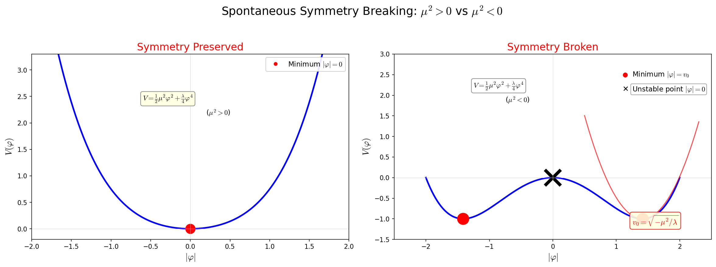
Fig. D.9: Potential for spontaneous symmetry breaking. Figure D_5: Left: With \(\mu^2 > 0\), the minimum is at the origin and symmetry is preserved. Right: With \(\mu^2 < 0\), the minimum moves away from the origin and the vacuum breaks the symmetry.
Here \(v\) is defined as:
\(v\) is called the vacuum expectation value (VEV). The physical minimum is \(|\phi|_{\text{min}} = v/\sqrt{2}\).
🔵 Kai: \(v\) and \(v/\sqrt{2}\) are confusing. Why does \(\sqrt{2}\) appear?
🟡 Lina: Good question. In the following calculations, we expand the field around the vacuum:
Here \(h(x)\) and \(\xi(x)\) are fluctuations from the vacuum (\(h = \xi = 0\) is the vacuum). Dividing by \(\sqrt{2}\) is a standard convention so that the kinetic terms of \(h\) and \(\xi\) take a clean form (\(\frac{1}{2}(\partial_\mu h)^2\), etc.). With this notation, at the vacuum (\(h = \xi = 0\)), \(|\phi| = v/\sqrt{2}\), which indeed matches the minimum we found.
⚪ Mei: So \(v\) is "a definition for writing the field expansion concisely," and the physical minimum is \(|\phi|_{\text{min}} = v/\sqrt{2}\).
🟡 Lina: Exactly. From here on, we'll use only \(v\) (\(v^2 = |\mu|^2/\lambda\)).
Now considering the shape of the potential: \(\phi = 0\) is a "hilltop" and \(|\phi| = v_0\) is the "valley bottom." Since \(\phi\) is complex, the points satisfying \(|\phi| = v_0\) form a circle in the complex plane. Comparing \(\mu^2 > 0\) (left) and \(\mu^2 < 0\) (right) in Fig. D.9 "Potential for spontaneous symmetry breaking", you can see the minimum position shifted from the origin. Furthermore, considering that \(\phi\) is complex and plotting in 3D with \(\text{Re}\,\phi\) and \(\text{Im}\,\phi\) axes, it takes the shape of a "Mexican hat (sombrero)" with a raised center (Fig. D.10 "Mexican hat potential"). You can see the minima arranged along the circle \(|\phi| = v/\sqrt{2}\).
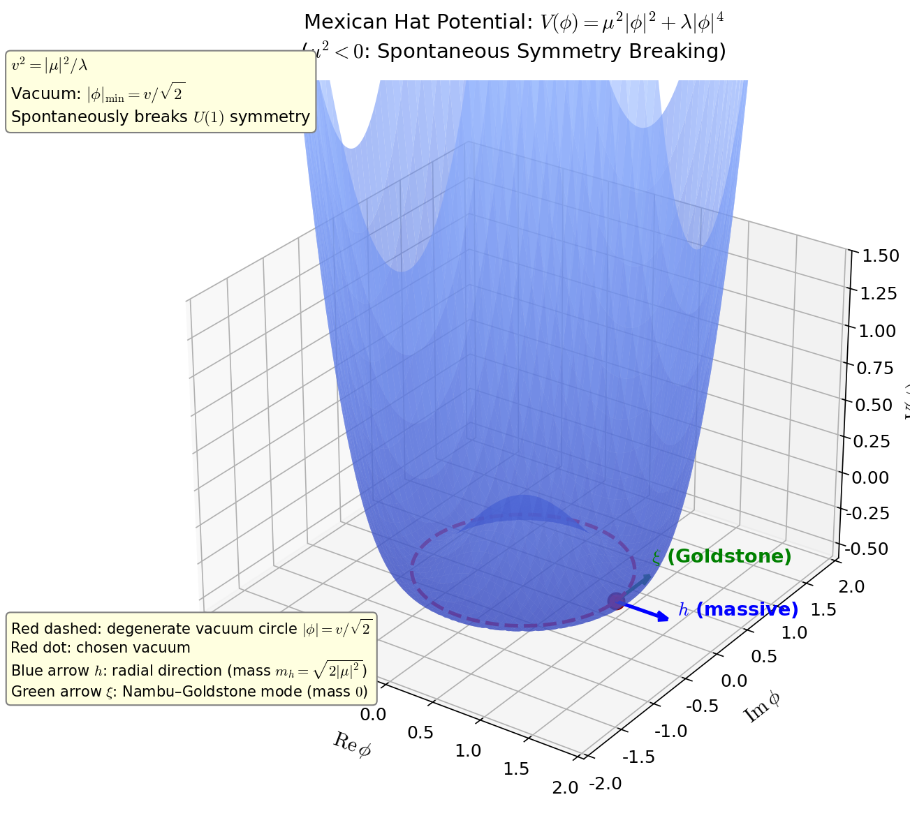
Fig. D.10: Mexican hat potential. The potential \(V(\phi) = \mu^2|\phi|^2 + \lambda|\phi|^4\) for \(\mu^2 < 0\), plotted in 3D with \(\text{Re}\,\phi\) and \(\text{Im}\,\phi\) axes. The center is raised, and the true minima lie along the circle \(|\phi| = v/\sqrt{2}\). The vacuum chooses one point on the circle, spontaneously breaking the \(U(1)\) symmetry.
Symmetry Breaking
The potential \(V(\phi)\) itself has \(U(1)\) symmetry (since \(|\phi|^2\) is invariant under \(\phi \to e^{i\alpha}\phi\), so is \(V\)).
However, the vacuum state chooses one specific point on the circle \(|\phi| = v/\sqrt{2}\). For example, suppose we choose \(\phi_0 = v/\sqrt{2}\) (a point on the real axis). This specific point moves under \(U(1)\) transformations, so the vacuum breaks the \(U(1)\) symmetry.
This is "spontaneous symmetry breaking":
- The law (Lagrangian) has the symmetry
- The state (vacuum) breaks the symmetry
Fluctuations Around the Vacuum — Goldstone Modes
Expand the field around the vacuum \(\phi_0 = v/\sqrt{2}\). Since we chose the vacuum on the real axis, decompose \(\phi\) into real and imaginary parts:
When \(h = \xi = 0\), \(\phi = v/\sqrt{2}\) (real), which matches the chosen vacuum. \(h(x)\) is the "radial direction" fluctuation (changing \(|\phi|\)) from the vacuum, and \(\xi(x)\) is the "circumferential direction" fluctuation (changing only the phase without changing \(|\phi|\)).
Substituting into the potential. Since \(|\phi|^2 = \frac{1}{2}[(v + h)^2 + \xi^2]\), substituting into \(V = -|\mu|^2|\phi|^2 + \lambda|\phi|^4\):
Let's expand using \(v^2 = |\mu|^2/\lambda\) (from the VEV definition). Setting \(\rho \equiv (v+h)^2 + \xi^2 = v^2 + 2vh + h^2 + \xi^2\):
Organizing \(\rho\) by powers of \(h\) and \(\xi\). Since \(\rho = v^2 + 2vh + (h^2 + \xi^2)\), let's find terms up to second order in \(h\) and \(\xi\). Setting \(A = v^2 + 2vh\), \(B = h^2 + \xi^2\), we have \(\rho = A + B\) and \(\rho^2 = A^2 + 2AB + B^2\). \(B^2\) is fourth order or higher, so ignore it.
\(A^2 = (v^2 + 2vh)^2 = v^4 + 4v^3 h + 4v^2 h^2\)
\(2AB = 2(v^2 + 2vh)(h^2 + \xi^2)\) expands to \(2v^2(h^2 + \xi^2) + 4vh(h^2 + \xi^2)\). The first term is second order in \(h\) and \(\xi\); the second term contains \(h \cdot h^2 = h^3\) and \(h \cdot \xi^2\), which are third order or higher, so ignore them in the second-order approximation. Thus the second-order part is \(2v^2(h^2 + \xi^2)\).
Combining the \(h^2\) coefficients: \(4v^2 + 2v^2 = 6v^2\); the \(\xi^2\) coefficient is \(2v^2\). So up to second order:
Substituting into \(V\):
Constant term (\(h = \xi = 0\)): \(-\frac{|\mu|^2}{2}v^2 + \frac{\lambda}{4}v^4\) (the vacuum energy, doesn't affect physics).
Linear term (proportional to \(h\)): \(-|\mu|^2 v h + \lambda v^3 h = vh(-|\mu|^2 + \lambda v^2) = 0\) (vanishes due to the vacuum condition \(v^2 = |\mu|^2/\lambda\). This reflects that "we're at the minimum").
⚪ Mei: The linear term being zero is because "being at the valley bottom means the slope is zero."
🟡 Lina: Exactly. Let's look at the quadratic terms:
Substituting \(v^2 = |\mu|^2/\lambda\):
So:
🔵 Kai: Huh, \(h^2\) has \(|\mu|^2\) in front, but \(\xi^2\) has \(0\). Does that mean something?
🟡 Lina: Absolutely. In field theory, the Lagrangian of a real scalar field takes the form \(\mathcal{L} = \frac{1}{2}(\partial_\mu h)^2 - \frac{1}{2}m^2 h^2 - \cdots\), where the mass term is written as \(\frac{1}{2}m^2 h^2\) (\(\frac{1}{2}\) pairs with the kinetic term \(\frac{1}{2}(\partial_\mu h)^2\) as a standard normalization). In our case, we expanded \(\phi = (v + h + i\xi)/\sqrt{2}\), so expanding the original kinetic term \((\partial_\mu\phi)^*(\partial^\mu\phi)\) gives—since \(\partial_\mu\phi = (\partial_\mu h + i\partial_\mu\xi)/\sqrt{2}\)—\((\partial_\mu\phi)^*(\partial^\mu\phi) = \frac{1}{2}(\partial_\mu h)^2 + \frac{1}{2}(\partial_\mu\xi)^2\), and the kinetic terms for \(h\) and \(\xi\) indeed have the standard \(\frac{1}{2}\) normalization.
🔵 Kai: So by reading the quadratic coefficient in the potential, you can determine the particle mass of that field?
🟡 Lina: Exactly. Generally, a field's Lagrangian is written as the difference of kinetic and potential terms: \(\mathcal{L} = \frac{1}{2}(\partial_\mu h)^2 - V\). It's the same structure as writing \(\frac{1}{2}m\dot{x}^2 - \frac{1}{2}kx^2\) in spring mechanics. The mass term appears in the Lagrangian as \(-\frac{1}{2}m^2 h^2\) (or \(+\frac{1}{2}m^2 h^2\) in the potential). The field's equation of motion becomes \(\ddot{h} + m^2 h = 0\), where \(m\) corresponds to the particle's mass.
🔵 Kai: That's like how in a spring \(\ddot{x} + (k/m)x = 0\) the frequency is \(\omega = \sqrt{k/m}\)—same structure. For fields, the "spring constant" equivalent is \(m^2\), which determines the particle mass.
🟡 Lina: Right, good analogy. Our result \(V^{(2)} = |\mu|^2 h^2\) is the quadratic term in the potential. The field Lagrangian is \(\mathcal{L} = \frac{1}{2}(\partial_\mu h)^2 - V\), so writing out the \(h\)-related part:
The standard free-field Lagrangian with mass \(m_h\) is \(\frac{1}{2}(\partial_\mu h)^2 - \frac{1}{2}m_h^2 h^2\), so the potential part is \(V = \frac{1}{2}m_h^2 h^2\). Comparing with our result \(V^{(2)} = |\mu|^2 h^2\) gives \(\frac{1}{2}m_h^2 = |\mu|^2\), i.e.:
🔵 Kai: \(\xi\)'s mass is zero! \(h\) has mass, but only \(\xi\) is massless.
🟡 Lina: This is the Goldstone theorem: when a continuous symmetry is spontaneously broken, a massless particle (Goldstone boson) appears for each broken generator.
The fact that \(\xi\) is massless can also be understood intuitively. Moving along the valley bottom of the Mexican hat (circumferential direction) costs no energy (the potential is flat). Moving away from the valley bottom (radial direction) requires energy.
🔵 Kai: I see, "where you are on the valley bottom" doesn't affect physics, so moving there costs nothing. That's why a massless particle appears. But wait, there aren't that many massless particles found in the real world, right? If a massless particle appears every time a symmetry breaks, there should be more.
🟡 Lina: Good question. Actually, when a gauge symmetry breaks, the story changes. That leads to the Higgs mechanism next.
✅ Comprehension Check: What does the Goldstone theorem state?
Answer
When a continuous symmetry is spontaneously broken, a massless particle (Goldstone boson) appears for each broken generator. It corresponds to fluctuations along the flat direction at the valley bottom of the Mexican hat.
Bridge to the Higgs Mechanism
🟡 Lina: As we'll see in detail in Ch. 9, when a gauge symmetry is spontaneously broken, the situation changes. The Goldstone boson \(\xi\) gets "eaten" by the gauge field, and the gauge field acquires mass. This is the Higgs mechanism.
In the Standard Model: - Of the 4 generators of \(SU(2) \times U(1)\), 3 are broken → 3 Goldstone bosons - These are eaten by the \(W^+\), \(W^-\), \(Z\) bosons, which acquire mass - The remaining 1 generator is unbroken → the photon remains massless - The radial fluctuation \(h\) is the Higgs particle (discovered in 2012)
✅ Comprehension Check: What happens to the Goldstone bosons in the Higgs mechanism?
Answer
The Goldstone bosons are "eaten" by the gauge fields and disappear; in exchange, the gauge fields (\(W^+\), \(W^-\), \(Z\) bosons) acquire mass. The radial fluctuation remains as the Higgs particle.
✅ Comprehension Check: What is spontaneous symmetry breaking? Explain using the pencil analogy.
Answer
The laws (equations) possess symmetry, but the realized state chooses a specific direction. A standing pencil could fall in any direction (symmetric), but when it actually falls, it chooses one direction (symmetry is broken).
✅ Comprehension Check: In the Mexican hat potential \(V = \mu^2|\phi|^2 + \lambda|\phi|^4\) (\(\mu^2 < 0\)), what is the vacuum expectation value \(|\phi|_{\text{min}}\)?
Answer
\(|\phi|_{\text{min}} = \sqrt{|\mu|^2/(2\lambda)}\). Obtained by differentiating the potential with respect to \(|\phi|\) and setting it to zero. In the notation of the text, defining \(v = \sqrt{|\mu|^2/\lambda}\), this can also be written as \(|\phi|_{\text{min}} = v/\sqrt{2}\).
D.9 Practice Problems
📝 Exercises:
- Verifying commutation relations of \(SU(2)\) generators → Problem B-6. Commutation Relation of Pauli Matrices \([\sigma_1, \sigma_2]\), Problem B-7. Commutation Relations of Pauli Matrices (All Pairs)
- Verifying group conditions → Problem B-1. Additive Group of Integers, Problem B-2. Multiplicative Group of Positive Real Numbers, Problem B-3. Multiplication of Integers Does Not Form a Group
- Verifying \(U(1)\) group conditions → Problem B-4. Group Conditions of \(U(1)\)
- Derivation of the number of parameters of \(SU(N)\) → Problem M-3. Parameter Count of \(SU(N)\)
- Computing an \(SU(2)\) element from Pauli matrices → Problem M-1. Exponential Representation of \(SU(2)\) Elements
- Composition rules for 3D rotation matrices → Problem B-5. 3-Dimensional \(z\)-Axis Rotation
- Eigenvalues and eigenvectors of spin \(1/2\) → Problem B-9. Eigenvalues and Eigenvectors of Spin 1/2
- Antisymmetry of commutators and Jacobi identity → Problem B-8. Antisymmetry of the Commutator, Problem M-2. Jacobi Identity (Verification with Pauli Matrices)
Preview of Next Chapter
The worldsheet of string theory is 2-dimensional, and the physics there is beautifully described in the language of complex analysis. Holomorphic functions, the residue theorem, conformal mappings—these tools form the mathematical foundation supporting conformal field theory and the operator product expansion (OPE) in Ch. 16. In Appendix E, we'll develop the core of complex analysis by the shortest route.
References
- M. Nakahara, Geometry, Topology and Physics, Ch.5 "Lie groups and Lie algebras" — Mathematical foundations of group theory
- Quantum Field Theory (Vol. 1), Ch.7 "The gauge principle" — Foundations of gauge symmetry, \(U(1)\) gauge theory
- Quantum Field Theory (Vol. 2), Ch.14 "Spontaneous symmetry breaking" — Mathematics of SSB, Goldstone's theorem
- Quantum Field Theory (Vol. 2), Ch.15 "The Standard Model and the Higgs mechanism" — Details of \(SU(3) \times SU(2) \times U(1)\)
- Quantum Mechanics Chapter 26 "Symmetry and conservation laws" — Quantum mechanical version of Noether's theorem
- Quantum Field Theory Chapter 3 "Classical field theory" — Field theory version of Noether's theorem
- Quantum Field Theory Chapter 17 "Yang-Mills theory" — Details of non-abelian gauge symmetry
- Quantum Field Theory Appendix B "Representation theory of the Lorentz and Poincaré groups" — Details of the Lorentz group
Feedback on this page
Let us know if something was unclear, incorrect, or could be improved.