Chapter 7: Interactions and the S-Matrix — How to Mix Fields
Story so far:
In Ch. 6, we tackled the quantization of the electromagnetic field. We faced the new difficulty of gauge freedom, and after applying the prescription of gauge fixing, confirmed that photons are quantized as transverse waves with 2 physical polarization degrees of freedom. This completed our quantization of free fields — scalar fields, Dirac fields, and electromagnetic fields.
Goals of this chapter
- Leave the world of free fields and introduce "interactions" where particles scatter off each other into quantum field theory
- Acquire the tools of the interaction picture, S-matrix, Dyson series, and Wick's theorem, and become able to concretely calculate the 2→2 scattering amplitude in \(\phi^4\) theory at lowest order
7.1 Why Interactions Are Necessary — The Boring World of Free Fields
🟡 Lina: From Ch. 4 through Ch. 6, we've quantized scalar fields, Dirac fields, and electromagnetic fields. But the theory so far has a serious flaw. What do you think it is?
🔵 Kai: Umm... particles don't collide?
🟡 Lina: Exactly right. Recall the free field Hamiltonian. For the scalar field case:
🟡 Lina: (where \(\omega_{\mathbf{p}} = \sqrt{|\mathbf{p}|^2 + m^2}\), normal-ordered). This \(\hat{H}_0\) commutes with the particle number operator \(\hat{N} \propto \int d^3p\, \hat{a}_{\mathbf{p}}^\dagger \hat{a}_{\mathbf{p}}\) —
Since both are (weighted) sums of the particle number operator \(\hat{a}_{\mathbf{p}}^\dagger \hat{a}_{\mathbf{p}}\) for each momentum mode, it's intuitively clear that they commute with each other.
⚪ Mei: So that means particle number doesn't change even under time evolution.
🟡 Lina: Right. Since particle number is conserved, neither scattering nor decay can occur. In the world of free fields, particles just fly in straight lines. Even if two electrons approach each other, they pass right through. But in the real world, when you collide protons in an accelerator, hundreds of particles come flying out, and radioactive nuclei decay. To describe such phenomena, we must add interaction terms to the Lagrangian. I've illustrated this difference in Fig. 7.1 "Comparison of time evolution for free and interacting fields".
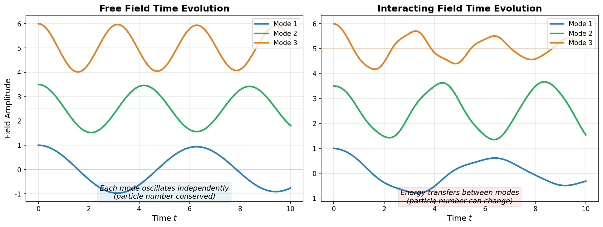
Fig. 7.1: Comparison of time evolution for free and interacting fields. In free fields, each mode oscillates independently and particle number is conserved, but in interacting fields, energy transfers between modes and particle number can change.
Splitting the Lagrangian — Free Part and Interaction Part
🟡 Lina: We split the Lagrangian density describing the fields into two parts:
- \(\mathcal{L}_0\): The free field part. The terms we've been dealing with in Chapters 3–6, containing at most quadratic products of fields (up to \(\phi^2\) for scalar fields, up to \(\bar{\psi}\psi\) for Dirac fields). Exactly solvable by canonical quantization.
- \(\mathcal{L}_{\text{int}}\): The interaction part. Describes forces between particles. When this is present, exact solutions can no longer be obtained.
✅ Comprehension Check: The conservation of particle number (no scattering occurs) under the free Hamiltonian \(\hat{H}_0\) is expressed mathematically by what condition?
Answer
\([\hat{H}_0,\, \hat{N}] = 0\), i.e., the free Hamiltonian and the particle number operator commute. As long as this commutation relation holds, particle number does not change under time evolution.
🔵 Kai: What does it look like concretely?
🟡 Lina: As the simplest example, let's consider the \(\phi^4\) theory (phi-four theory) of a real scalar field.
Here \(\lambda\) is a parameter called the coupling constant, which determines the "strength" of the interaction. In natural units (\(\hbar = c = 1\)), the action \(S = \int d^4x\, \mathcal{L}\) must be dimensionless. This condition determines the dimension of \(\lambda\), but first let me organize how we count "dimensions."
In natural units we set \(\hbar = c = 1\), so the exponent \(S/\hbar\) appearing in the quantum mechanical probability amplitude \(e^{iS/\hbar}\) must be dimensionless — the quantity in the exponent of an exponential must be a "pure number" (you can't write \(e^{3\text{kg}}\), right?). Since \(\hbar = 1\), \(S\) itself must be dimensionless (\([S] = 0\)). Incidentally, \(e^{iS/\hbar}\) appears as the "weight" for each path in a formulation called the path integral, but we'll cover that in detail in a later chapter. For now, we'll just use the conclusion that "the action \(S\) must be dimensionless."
🔵 Kai: I see, since it sits in the exponent of \(e\), it has to be dimensionless.
🟡 Lina: Right. Next, from the dispersion relation \(E^2 = p^2 + m^2\) (with \(c = 1\)), we have \([E] = [p] = [m]\). Also from \(p = \hbar k\) (with \(\hbar = 1\)), we get \([p] = [k]\). Since the wavenumber \(k\) is the inverse of wavelength \(\lambda\) (\(k = 2\pi/\lambda\)), it has the dimension of inverse length — that is, \([k] = [1/\text{length}]\). Since this equals \([m]\), the dimension of length is the inverse of mass: \([\text{length}] = [m]^{-1}\). Similarly, from \(c = 1\) (\(c = \text{length}/\text{time}\)), we get \([\text{time}] = [\text{length}] = [m]^{-1}\). So energy, momentum, and mass all have the same dimension, while length and time have the dimension of inverse mass. This means we can express the dimensions of all quantities using mass alone as the reference.
Let me introduce a convenient notation. When we write \([A]\), it means "the mass dimension of \(A\)" — that is, the integer (or rational number) representing "what power of mass does \(A\) have as its dimension." For example, writing \([x^\mu] = -1\) means "the dimension of \(x^\mu\) is mass to the power \(-1\) (= inverse mass)."
⚪ Mei: In programming terms, it's like expressing all physical quantities uniformly in a single type of "what power of mass."
🟡 Lina: Nice analogy. The mass dimension of a product is the sum of the mass dimensions of each factor — \([AB] = [A] + [B]\). You might wonder "a product gives a sum?" but it's the same as the exponent rule \(m^a \times m^b = m^{a+b}\) you learned in high school. Since \([\cdot]\) represents the "power (exponent)" of "what power of mass," when you multiply quantities, the "powers" add up. For example, if \([A] = 2\) (dimension of \(A\) is mass\(^2\)) and \([B] = 1\) (dimension of \(B\) is mass\(^1\)), then the dimension of \(AB\) is mass\(^2 \times\) mass\(^1\) = mass\(^{2+1}\) = mass\(^3\), so \([AB] = 2 + 1 = 3\). For quotients it's subtraction — \([A/B] = [A] - [B] = 2 - 1 = 1\).
Let me work through things step by step using this. - \(d^4x = dx^0\,dx^1\,dx^2\,dx^3\) is the product of infinitesimal amounts of 4 coordinates. Each \(dx^\mu\) has the same dimension as the coordinate \(x^\mu\), so \([dx^\mu] = [x^\mu] = -1\). Using the product rule \([AB] = [A] + [B]\) four times: \([d^4x] = [dx^0] + [dx^1] + [dx^2] + [dx^3] = 4 \times (-1) = -4\) - For the action \(S\) to be dimensionless (\([S] = 0\)), we need \([\mathcal{L}] + [d^4x] = 0\), i.e., \([\mathcal{L}] = 4\) - Derivatives have dimension of inverse length, so \([\partial_\mu] = 1\) - The dimension of the free kinetic term \(\frac{1}{2}\partial_\mu\phi\,\partial^\mu\phi\) is \([\partial_\mu\phi\,\partial^\mu\phi] = 2(1 + [\phi]) = 4\), giving \([\phi] = 1\) - \([\lambda \phi^4] = [\lambda] + 4[\phi] = [\lambda] + 4 = 4\), giving \([\lambda] = 0\) — meaning \(\lambda\) is dimensionless
🔵 Kai: Huh, so \(\lambda\) has no units. Then it really is a pure number representing just the "strength."
🟡 Lina: Exactly. Dividing by \(4!\) is a convention that makes combinatorial factors come out cleanly in later calculations. Specifically, when we calculate 2→2 scattering later in this chapter, the \(4! = 24\) combinations arising from expanding \(\hat{\phi}^4\) will exactly cancel the \(4!\) in the denominator — you'll see the "aha" moment there.
⚪ Mei: If \(\lambda\) is small, then the effect of interactions is also small, so we can treat it approximately.
🟡 Lina: Exactly. When \(\lambda \ll 1\), we systematically expand the "deviation" from the free field in powers of \(\lambda\) — this is perturbation theory.
✅ Comprehension Check: When splitting the Lagrangian density as \(\mathcal{L} = \mathcal{L}_0 + \mathcal{L}_{\text{int}}\), what role does each of \(\mathcal{L}_0\) and \(\mathcal{L}_{\text{int}}\) play?
Answer
\(\mathcal{L}_0\) is the free field part, consisting of terms up to quadratic in the fields, and is exactly solvable by canonical quantization. \(\mathcal{L}_{\text{int}}\) is the interaction part, describing forces between particles. When \(\mathcal{L}_{\text{int}}\) is present, exact solutions cannot be obtained, so when the coupling constant is small, it is treated approximately using perturbation theory.
What Does the \(\phi^4\) Interaction Do?
🔵 Kai: \(\phi^4\) just means multiplying the field four times, right? How does that become "particles colliding"?
🟡 Lina: Good question. When you expand the field \(\hat{\phi}\) in creation and annihilation operators, schematically \(\hat{\phi} \sim \hat{a} + \hat{a}^\dagger\), right? So \(\hat{\phi}^4\) contains terms like
In reality, each operator carries a different momentum label, so for example \(\hat{a}_{\mathbf{p}_3}^\dagger \hat{a}_{\mathbf{p}_4}^\dagger \hat{a}_{\mathbf{p}_1}\, \hat{a}_{\mathbf{p}_2}\) means "annihilate particles with momenta \(\mathbf{p}_1, \mathbf{p}_2\) and create particles with momenta \(\mathbf{p}_3, \mathbf{p}_4\)" — describing 2-particle scattering. I've summarized representative combinations and their corresponding physical processes in Table 7.1 "Representative operator combinations in \(\hat{\phi}^4\) and their corresponding physical processes".
Table 7.1: Representative operator combinations in \(\hat{\phi}^4\) and their corresponding physical processes
| Operator type | Physical process | Particle number change |
|---|---|---|
| \(\hat{a}^\dagger\hat{a}^\dagger\hat{a}\,\hat{a}\) | 2→2 scattering | \(\Delta N = 0\) |
| \(\hat{a}^\dagger\hat{a}^\dagger\hat{a}^\dagger\hat{a}\) | 1→3 splitting | \(\Delta N = +2\) |
| \(\hat{a}^\dagger\hat{a}\,\hat{a}\,\hat{a}\) | 3→1 fusion | \(\Delta N = -2\) |
| \(\hat{a}^\dagger\hat{a}^\dagger\hat{a}^\dagger\hat{a}^\dagger\) | 0→4 particle creation from vacuum | \(\Delta N = +4\) |
| \(\hat{a}\,\hat{a}\,\hat{a}\,\hat{a}\) | 4→0 particle annihilation into vacuum | \(\Delta N = -4\) |
🔵 Kai: I see, so the combinations of creation and annihilation operators represent particles going in and out. But terms like \(\hat{a}^\dagger\hat{a}^\dagger\hat{a}^\dagger\hat{a}\) — "create 3 and annihilate 1" — are also there, right? Does that mean one particle splits into three? But it seems like one particle suddenly becoming three would violate energy conservation...
🟡 Lina: Yes, in principle such processes are included in \(\hat{H}_{\text{int}}\). However, whether they actually occur is restricted by energy-momentum conservation. For example, for one particle of mass \(m\) to split into three particles of mass \(m\), you need at least energy \(3m\), but a particle at rest only has energy \(m\) — so it can't happen in free space. However, it can be allowed as a virtual process (intermediate state). Today we'll focus on 2→2 scattering, but allowing processes that change particle number is an essential feature of quantum field theory.
🔵 Kai: But wait. If terms that change particle number are in the Hamiltonian, then the \([\hat{H}_0, \hat{N}] = 0\) we saw earlier no longer holds...?
🟡 Lina: Exactly. Since \(\hat{H}_{\text{int}}\) contains operators that change particle number, \([\hat{H}, \hat{N}] \neq 0\). Processes that change particle number are now allowed. But there's a problem. The Hamiltonian with interactions \(\hat{H} = \hat{H}_0 + \hat{H}'\) can no longer be diagonalized. That is, exact solutions cannot be obtained.
🔵 Kai: Since we can't solve it exactly, we have no choice but to approximate... but how small does \(\lambda\) need to be specifically for the approximation to be trustworthy? Is there a criterion like "\(\lambda = 0.1\) is fine but \(\lambda = 0.5\) is not"?
🟡 Lina: Good question. The strict criterion depends on the problem, but the basic guideline is that "the \(n\)-th order correction must be sufficiently small compared to the \((n-1)\)-th order." In \(\phi^4\) theory, since \(\lambda\) is dimensionless, if \(\lambda \ll 1\) then higher-order terms decrease rapidly as \(\lambda^n\), and you get a good approximation from just the first few orders. Conversely, if \(\lambda \gg 1\), perturbation theory breaks down — the low-energy regime of QCD is exactly such a case, requiring other methods (like lattice calculations).
⚪ Mei: So the condition for perturbation theory to work is "that \(\lambda\) is small" — specifically, that higher-order terms become negligibly small compared to the previous order.
🟡 Lina: Right. But for today, let's focus on the case \(\lambda \ll 1\). We'll now build the method for calculating approximately using perturbation theory. For that, we first introduce a new framework called the interaction picture — within which we'll also derive the specific form of the interaction Hamiltonian \(\hat{H}'\) (in particular, the sign relation with the Lagrangian: \(\hat{H}' = -\int d^3x\,\mathcal{L}_{\text{int}}\)).
✅ Comprehension Check: What is the mass dimension of the coupling constant \(\lambda\) in \(\phi^4\) theory? (Hint: use \([\mathcal{L}] = 4\), \([\phi] = 1\) in natural units)
Answer
\([\lambda/4! \cdot \phi^4] = [\lambda] + 4[\phi] = [\lambda] + 4 = 4\), giving \([\lambda] = 0\). That is, \(\lambda\) is dimensionless. Such an interaction is called marginal.
7.2 The Interaction Picture — "Division of Labor" Between Operators and States
🟡 Lina: To proceed with perturbative calculations, we'll introduce a new "picture." Do you remember the discussion of pictures from Quantum Mechanics Ch. 13?
🔵 Kai: In the Schrödinger picture, states evolve in time and operators are fixed; in the Heisenberg picture, it's the opposite... right? The Schrödinger equation \(i\frac{d}{dt}|\psi\rangle = \hat{H}|\psi\rangle\) moves the state in the Schrödinger picture, and the thinking "since the expectation value \(\langle\psi|\hat{O}|\psi\rangle\) is the same, fixing the state and instead making the operators time-dependent shouldn't change the physics" — that's how you transfer the time evolution to the operator side in the Heisenberg picture. The third "interaction picture" was introduced in Quantum Mechanics Ch. 13, but at that time it was just a conceptual introduction and we didn't use it for concrete calculations, right?
🟡 Lina: Right. Here we'll put that third option — the interaction picture, also called the Dirac picture — to serious use. We'll apply the concept introduced in Quantum Mechanics Ch. 13 to scattering problems in quantum field theory.
Splitting the Hamiltonian and Defining the Picture
🟡 Lina: The starting point is splitting the Hamiltonian into two parts.
Here \(\hat{H}' = -\int d^3x\, \mathcal{L}_{\text{int}}\) is the interaction Hamiltonian (I'll derive the origin of this sign just below). Note that \(\hat{H}'\) is the interaction Hamiltonian in the Schrödinger picture. In the Schrödinger picture, operators (including fields) are time-independent constants, so \(\hat{H}'\) is also time-independent. The \(\hat{H}_I(t) = e^{i\hat{H}_0 t}\hat{H}'e^{-i\hat{H}_0 t}\) that appears later is this transferred to the interaction picture — meaning "rotated" by \(\hat{H}_0\) to give it time dependence.
🔵 Kai: Why does a minus sign appear? Are Lagrangians and Hamiltonians opposite in sign?
🟡 Lina: As we learned in Ch. 3, the Hamiltonian density is defined through a Legendre transformation — an operation that changes the independent variable from "velocity" \(\dot{\phi}\) to "momentum" \(\pi\) — as \(\mathcal{H} = \pi\dot{\phi} - \mathcal{L}\). Here \(\pi = \partial\mathcal{L}/\partial\dot{\phi}\) is the canonical momentum density — a quantity measuring the Lagrangian's response to the field "velocity" \(\dot{\phi}\), the field theory version of \(p = \partial L/\partial\dot{q}\) from particle mechanics. The sign reversal between \(L\) and \(H\) comes from this Legendre transformation structure — \(H = p\dot{q} - L\). Substituting \(\mathcal{L} = \mathcal{L}_0 + \mathcal{L}_{\text{int}}\) gives
Here we can write \(\pi\dot{\phi} - \mathcal{L}_0 = \mathcal{H}_0\) because when \(\mathcal{L}_{\text{int}}\) doesn't contain \(\dot{\phi}\), the canonical momentum is determined by the free field alone: \(\pi = \partial\mathcal{L}_0/\partial\dot{\phi}\).
🔵 Kai: Ah, since \(\mathcal{L}_{\text{int}} = -\frac{\lambda}{4!}\phi^4\) doesn't contain the time derivative \(\dot{\phi}\), it doesn't affect the canonical momentum.
🟡 Lina: Exactly. Let's verify this concretely. Since \(\mathcal{L}_{\text{int}} = -\frac{\lambda}{4!}\phi^4\) in \(\phi^4\) theory doesn't contain \(\dot{\phi}\), we get \(\pi = \partial\mathcal{L}/\partial\dot{\phi} = \partial(\mathcal{L}_0 + \mathcal{L}_{\text{int}})/\partial\dot{\phi} = \partial\mathcal{L}_0/\partial\dot{\phi} = \dot{\phi}\). So the relationship between \(\pi\) and \(\dot{\phi}\) doesn't change with or without the interaction, meaning \(\pi\dot{\phi} - \mathcal{L}_0\) is precisely the free field Hamiltonian density \(\mathcal{H}_0\).
Therefore \(\mathcal{H}_{\text{int}} = -\mathcal{L}_{\text{int}}\). Since the Hamiltonian is the spatial integral of the Hamiltonian density, \(\hat{H}' = \int d^3x\, \mathcal{H}_{\text{int}} = -\int d^3x\, \mathcal{L}_{\text{int}}\). If \(\mathcal{L}_{\text{int}}\) contains \(\dot{\phi}\), this clean separation doesn't work, but the interaction term \(-\frac{\lambda}{4!}\phi^4\) in \(\phi^4\) theory doesn't contain \(\dot{\phi}\), so this condition is satisfied.
⚪ Mei: I see, so \(\hat{H}'\) is obtained by attaching a minus sign to \(\mathcal{L}_{\text{int}}\) and integrating over space.
🟡 Lina: Right. Now let me state the definition of the interaction picture. In this picture:
- Operators evolve in time according to the free Hamiltonian \(\hat{H}_0\)
- States evolve in time according to the interaction Hamiltonian \(\hat{H}_I(t)\)
Specifically, we define operators in the interaction picture as
(\(\hat{O}_S\) is the operator in the Schrödinger picture, a time-independent constant operator. Using natural units \(\hbar = 1\)).
⚪ Mei: In the Heisenberg picture it was \(\hat{O}_H(t) = e^{i\hat{H} t}\, \hat{O}_S\, e^{-i\hat{H} t}\), so instead of the full Hamiltonian \(\hat{H}\), we're evolving with just the free part \(\hat{H}_0\).
🟡 Lina: Exactly.
Equation of Motion for Operators
✅ Comprehension Check: How does the definition of the interaction picture operator \(\hat{O}_I(t)\) in equation (7.2) differ from the definition of operators in the Heisenberg picture?
Answer
In the Heisenberg picture, operators are evolved in time using the full Hamiltonian \(\hat{H} = \hat{H}_0 + \hat{H}'\) (\(\hat{O}_H(t) = e^{i\hat{H}t}\hat{O}_S e^{-i\hat{H}t}\)), whereas in the interaction picture, they are evolved using only the free part \(\hat{H}_0\) (\(\hat{O}_I(t) = e^{i\hat{H}_0 t}\hat{O}_S e^{-i\hat{H}_0 t}\)).
🟡 Lina: Let's differentiate equation (7.2) with respect to time.
That is,
🔵 Kai: Wait, only \(\hat{H}_0\) appears on the right-hand side. Where did the interaction \(\hat{H}'\) go?
🟡 Lina: Good question. The effect of the interaction is pushed into the state. What equation (7.3) means is that the field operators in the interaction picture \(\hat{\phi}_I(x)\) obey the free field equations of motion. So the mode expansion we learned in Ch. 4
Note that starting from this chapter, we change the mode expansion convention. In Chapter 4, we used \((2\pi)^{3/2}\) in the denominator with \([\hat{a}_{\mathbf{p}},\, \hat{a}_{\mathbf{q}}^\dagger] = \delta^{(3)}(\mathbf{p}-\mathbf{q})\), but for scattering problems the convention with \((2\pi)^3\) in the denominator
is more standard and has better compatibility with covariant normalization. The only difference is whether the \((2\pi)^3\) factor is absorbed into the denominator of the mode expansion or appears in the commutation relation — the physical results don't change. We'll use this convention from here on.
This mode expansion can be used as is. Commutation relations, propagators — all the results from free fields carry over directly.
⚪ Mei: So regarding operators, everything we've learned so far can be used as is. Incredibly convenient.
🔵 Kai: Um, you said we're changing conventions, but which convention are we using for the calculations that follow? I'm worried about getting confused...
🟡 Lina: Sorry, let me be clear. From this chapter onward, we consistently use the convention of equations (7.4) and (7.4a) — mode expansion with \((2\pi)^3\) in the denominator, commutation relation \([\hat{a}_{\mathbf{p}}, \hat{a}_{\mathbf{q}}^\dagger] = (2\pi)^3\delta^{(3)}(\mathbf{p}-\mathbf{q})\). We won't use the Chapter 4 convention (denominator \((2\pi)^{3/2}\), no \((2\pi)^3\) in the commutation relation) anymore, so don't worry.
✅ Comprehension Check: Why can the field operator \(\hat{\phi}_I(x)\) in the interaction picture use the free field mode expansion as is?
Answer
Since only \(\hat{H}_0\) appears on the right-hand side of the equation of motion (7.3) for interaction picture operators, \(\hat{\phi}_I(x)\) obeys the free field equation of motion (Klein-Gordon equation). Therefore, the mode expansion, commutation relations, and propagators derived for free fields all apply directly.
Time Evolution of States — Driven by \(\hat{H}_I(t)\)
🟡 Lina: Now, where does the effect of interactions appear? We define the state in the interaction picture \(|\psi_I(t)\rangle\) as
(\(|\psi(t)\rangle_S\) is the state in the Schrödinger picture). Let me derive the equation of motion for this state. Differentiating equation (7.5) with respect to time:
We expand the right-hand side using the product rule. Since \(\hat{H}_0\) is time-independent, \(\frac{d}{dt}e^{i\hat{H}_0 t} = i\hat{H}_0\, e^{i\hat{H}_0 t}\). Multiplying by the \(i\) from the left-hand side gives \(i \times i\hat{H}_0 = -\hat{H}_0\), so
Substituting the Schrödinger equation \(i\frac{d}{dt}|\psi(t)\rangle_S = \hat{H}\, |\psi(t)\rangle_S = (\hat{H}_0 + \hat{H}')\, |\psi(t)\rangle_S\):
Substituting \(|\psi(t)\rangle_S = e^{-i\hat{H}_0 t}\, |\psi_I(t)\rangle\):
where
🔵 Kai: Oh, so the time evolution of states is determined by the interaction Hamiltonian \(\hat{H}_I(t)\) alone! If there's no interaction (\(\hat{H}' = 0\)), the state doesn't change.
🟡 Lina: Exactly. Let me summarize the three pictures in a table.
Table 7.2: Comparison of Schrödinger, Heisenberg, and interaction pictures
| Picture | Time evolution of operators | Time evolution of states |
|---|---|---|
| Schrödinger | None | Evolves with \(\hat{H} = \hat{H}_0 + \hat{H}'\) |
| Heisenberg | Evolves with \(\hat{H}\) | None |
| Interaction | Evolves with \(\hat{H}_0\) | Evolves with \(\hat{H}_I(t)\) |
⚪ Mei: Operators can be treated as free fields, and changes in the state are driven only by the interaction. If there's no interaction, the state doesn't change at all — a formulation perfectly suited for scattering problems.
✅ Comprehension Check: In the interaction picture, what governs the time evolution of operators? What governs the time evolution of states?
Answer
Operators evolve in time according to the free Hamiltonian \(\hat{H}_0\). States evolve in time according to the interaction Hamiltonian \(\hat{H}_I(t) = e^{i\hat{H}_0 t}\hat{H}'e^{-i\hat{H}_0 t}\).
📝 Exercises:
- Derivation of the equation of motion for operators in the interaction picture → Problem M-1. Derivation of the Equation of Motion for States in the Interaction Picture
7.3 Definition of the S-Matrix — Connecting the "Entrance" and "Exit" of Scattering
🟡 Lina: Next, let's formulate scattering experiments. A typical scattering experiment has 3 stages:
- \(t \to -\infty\): Particles are sufficiently far apart and can be described as free particles (initial state \(|i\rangle\))
- Finite time: Particles collide and the interaction \(\hat{H}_I\) takes effect
- \(t \to +\infty\): After the reaction, particles separate again and can be described as free particles (final state \(|f\rangle\))
🔵 Kai: So both the initial and final states are free particles. The interaction only matters "in between."
🟡 Lina: Right. I've illustrated this 3-stage structure in Fig. 7.2 "The 3 stages of a scattering experiment and the S-matrix" (the \(\hat{U}_I\) and \(\hat{S}\) in the figure will be defined shortly). In the interaction picture, states evolve with \(\hat{H}_I\). Intuitively, when particles are sufficiently far apart at \(t \to \pm\infty\), the effect of interactions is negligible and the state is "frozen." These frozen states are precisely free particle states — eigenstates of \(\hat{H}_0\).
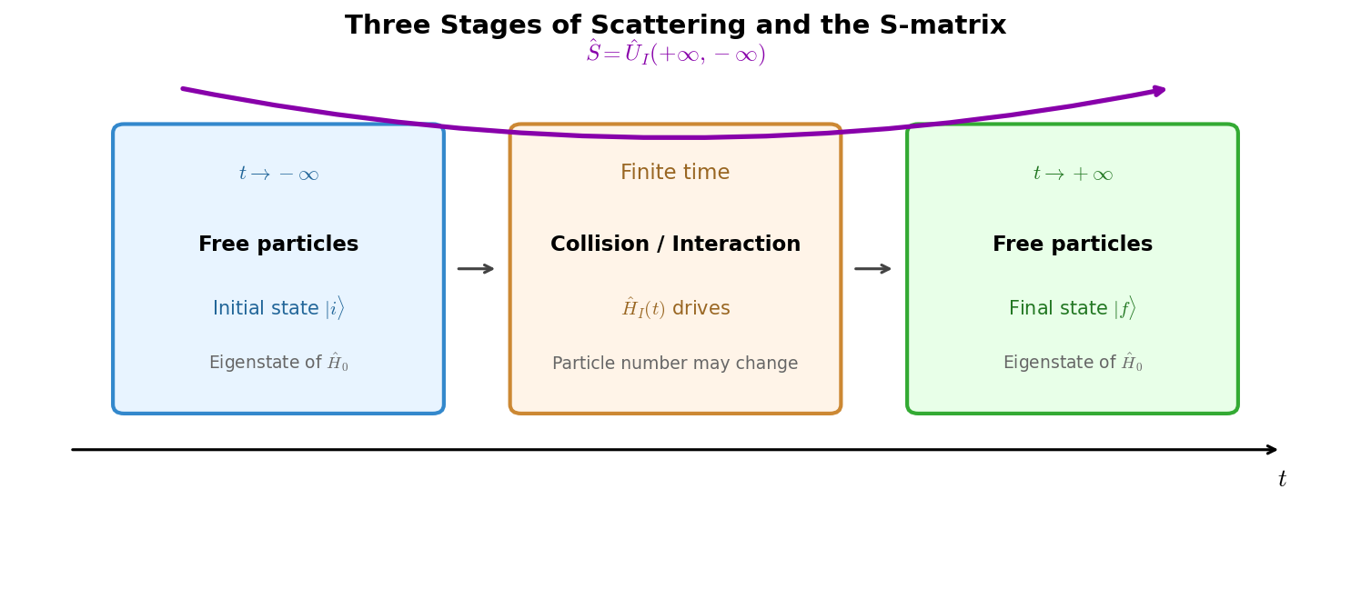
Fig. 7.2: The 3 stages of a scattering experiment and the S-matrix. In the distant past (\(t \to -\infty\)) and distant future (\(t \to +\infty\)), particles are free (eigenstates of \(\hat{H}_0\)), and the interaction \(\hat{H}_I(t)\) acts during finite time. The S-operator \(\hat{S} = \hat{U}_I(+\infty, -\infty)\) connects the initial and final states.
🔵 Kai: But looking at the formula for \(\hat{H}_I(t)\), it doesn't seem to automatically go to zero as \(t \to \pm\infty\)...
🟡 Lina: Sharp observation. Strictly speaking, we assume that the interaction is "switched off" slowly in the infinite past and future as \(e^{-\varepsilon|t|}\hat{H}_I(t)\) (where \(\varepsilon > 0\) is infinitesimal) — this is called adiabatic switching. \(e^{-\varepsilon|t|}\) is close to 1 near \(t = 0\) but decays to zero as \(|t| \to \infty\) — mathematically expressing that the interaction is "off" in the distant past and future.
🔵 Kai: So "slowly" is the key point. The reason you can't switch it on and off suddenly is...
🟡 Lina: Right, "slowly" is the key point — if you switch the interaction on and off suddenly, problems arise. Recall the property of Fourier transforms — the shorter a pulse of light, the wider the range of frequencies it contains (@chapter:qm/appendix_c). By the same principle, the more abruptly you switch the interaction on/off (shorter duration \(\Delta t\)), the wider the range of energy \(\Delta E\) injected into the system. This comes from the bandwidth relationship of Fourier transforms — the property we learned in @chapter:qm/appendix_c that "the shorter the pulse duration \(\Delta t\), the wider the range of frequencies \(\Delta\omega\)" (\(\Delta\omega \cdot \Delta t \gtrsim 1\)). In natural units (\(\hbar = 1\)), \(E = \hbar\omega = \omega\), so this can be written directly as \(\Delta E \cdot \Delta t \gtrsim 1\). If \(\Delta E\) exceeds the particle mass \(m\) (recall that in natural units, \(E = m\) is the minimum energy needed to create one particle), the excess energy can create new particles. If you switch sufficiently slowly (adiabatically), \(\Delta E \approx 0\) and the system transitions smoothly from the free particle state to the interacting state. Ultimately we take the limit \(\varepsilon \to 0\). Thanks to this prescription, we can treat the states at \(t \to \pm\infty\) as free particles. The rigorous justification is an advanced topic, so for now just think of it as "an established convention."
The Time Evolution Operator \(\hat{U}_I\)
🟡 Lina: Let's write the time evolution of states in the interaction picture using an operator \(\hat{U}_I(t, t_0)\).
Substituting into equation (7.6), \(\hat{U}_I\) satisfies
Definition of the S-Operator
🟡 Lina: The S in S-matrix stands for "scattering." The S-operator \(\hat{S}\) is defined as the time evolution operator in the limits \(t_0 \to -\infty\), \(t \to +\infty\).
The scattering amplitude is given by
Here \(|i\rangle\), \(|f\rangle\) are free particle states — eigenstates of \(\hat{H}_0\).
🔵 Kai: So \(|\langle f|\hat{S}|i\rangle|^2\) is the transition probability. Is it like a generalization of Fermi's golden rule from quantum mechanics?
🟡 Lina: Exactly. Fermi's golden rule is derived from the lowest-order approximation of the S-matrix. In quantum field theory, everything — including processes that change particle number — is encapsulated in \(\hat{S}\).
🔵 Kai: Wait, what if the initial state \(|i\rangle\) and final state \(|f\rangle\) are the same — that is, no scattering occurs? With \(|\langle f|\hat{S}|i\rangle|^2\), the probability of "nothing happening" would be included too, right?
🟡 Lina: Good question. To separate out the part where no scattering occurs, we often write \(\hat{S}\) as
\(\mathbb{1}\) is the "nothing happens" part, and \(i\hat{T}\) describes the transitions due to interactions. The \(i\) is a convention — with it, when we later define the invariant amplitude \(\mathcal{M}\), we can write \(\langle f|i\hat{T}|i\rangle = i\mathcal{M} \times (\text{delta function})\), and from the result of \(\hat{S}^{(1)}\) being \(-i\lambda \times (\text{delta function})\), we can directly read off \(\mathcal{M} = -\lambda\) — we'll actually verify this at the end of this chapter. The scattering cross sections that are actually measured are calculated from the matrix elements of \(\hat{T}\).
✅ Comprehension Check: What is the reason for decomposing the S-operator as \(\hat{S} = \mathbb{1} + i\hat{T}\)?
Answer
\(\mathbb{1}\) represents the part where no scattering occurs (initial and final states are the same), and \(i\hat{T}\) describes the actual transitions due to interactions. Since experimentally measured quantities like scattering cross sections are calculated from the matrix elements of \(\hat{T}\), it's convenient to separate out the "nothing happens" contribution.
✅ Comprehension Check: In the definition of the S-operator \(\hat{S} = \hat{U}_I(+\infty, -\infty)\), \(|i\rangle\) and \(|f\rangle\) are eigenstates of which Hamiltonian?
Answer
Eigenstates of the free Hamiltonian \(\hat{H}_0\). Before and after scattering, particles are sufficiently far apart that interactions don't take effect, so they can be described as free particles.
7.4 The Dyson Series — Perturbatively Expanding the S-Matrix
🟡 Lina: Let's find \(\hat{U}_I(t, t_0)\) concretely. Rearranging equation (7.9) gives \(\frac{\partial}{\partial t}\hat{U}_I(t, t_0) = -i\hat{H}_I(t)\hat{U}_I(t, t_0)\), and integrating both sides from \(t_0\) to \(t\):
Using the initial condition \(\hat{U}_I(t_0, t_0) = 1\):
This still has \(\hat{U}_I\) remaining on the right-hand side — the quantity we want to find is inside the integral. Such an equation is called an integral equation. For an algebraic equation like \(x = 1 + 0.1x\), you can rearrange to get \(x = 1/0.9\), but when the unknown function is trapped inside an integral sign like "\(f(t) = 1 + \int(\cdots f \cdots)\)," you can't "move \(f\) to the left side" because it's locked inside the integral — so we use iterative substitution to approximate.
🔵 Kai: I saw similar equations in quantum mechanics perturbation theory. You iterate the substitution to expand, right? But if you keep substituting infinitely, does it converge?
🟡 Lina: Good question. Since \(\hat{H}_I\) is proportional to the coupling constant \(\lambda\), the term obtained after \(n\) substitutions is proportional to \(\lambda^n\). If \(\lambda \ll 1\), higher-order terms become smaller, so truncating at finite order still gives a good approximation. This is the basic idea of perturbation theory. Now let me concretely substitute equation (7.13) itself into the \(\hat{U}_I(t_1, t_0)\) on the right-hand side.
0th order: \(\hat{U}_I^{(0)} = 1\)
1st order: Substitute 0th order into \(\hat{U}_I\) on the right:
2nd order: Substitute 1st order into \(\hat{U}_I\) on the right:
🔵 Kai: In the second-order term, why is the upper limit of integration \(t_1\) instead of \(t\)?
🟡 Lina: It comes from the structure of iterative substitution. We're substituting a further interaction at time \(t_2\) "inside" the interaction at time \(t_1\), so \(t_2\) must always be before \(t_1\) — the time ordering \(t_2 < t_1\) is automatically guaranteed.
⚪ Mei: I see, the causal ordering "interaction at \(t_2\) comes first, interaction at \(t_1\) comes after" is reflected in the integration limit.
🟡 Lina: Well caught, Mei. Here we use an important trick. Instead of restricting the integration region to \(t_0 \le t_2 \le t_1 \le t\), we introduce the time-ordered product \(T\) to free up the integration range.
Definition of the Time-Ordered Product \(T\)
🟡 Lina: Let me define the time-ordered product \(T\) for bosonic field operators.
That is, always place the later-time operator to the left. For the case \(t_1 = t_2\), bosonic fields at equal times but different spatial points commute (the equal-time commutation relation \([\hat{\phi}(t,\mathbf{x}),\, \hat{\phi}(t,\mathbf{y})] = 0\) we learned in Ch. 4), so the result is the same regardless of ordering.
🔵 Kai: Why is the right side "earlier"?
🟡 Lina: As we learned in Quantum Mechanics Ch. 13, operators act on states from the right. When you write \(\hat{A}(t_1)\hat{B}(t_2)|i\rangle\), first the rightmost \(\hat{B}(t_2)\) acts on \(|i\rangle\), then \(\hat{A}(t_1)\) acts on the result. So to "apply what happened first (\(t_2\) is earlier) first," we need to place the earlier operator on the right. The time-ordered product automatically incorporates this causal ordering — cause comes first, effect comes after.
🔵 Kai: What about the case of fermions? Since there are anticommutation relations, something should change...
🟡 Lina: Good intuition. As we learned in Ch. 5, fermionic fields satisfy anticommutation relations \(\{\hat{\psi}, \hat{\psi}\} \neq 0\), so each time operators are swapped, a minus sign appears. So in the time-ordered product too, each swap produces a \((-1)\). The formal definition of the time-ordered product for fermions will be given when we calculate QED scattering in Ch. 8 and beyond. For now we're focusing on bosonic scalar fields, so there's no sign to worry about.
✅ Comprehension Check: Why does the time-ordered product \(T\) "place later-time operators to the left"? State the physical meaning.
Answer
Since operators act on states from the right, the rightmost operator acts first. The time-ordered product arranges things so that "interactions that happened first are applied first," naturally incorporating causality — cause comes first, effect comes after.
The Dyson Series Using the Time-Ordered Product
🟡 Lina: Using the time-ordered product, the second-order term can be rewritten as follows.
Consider the integration region of \((t_1, t_2)\) as a square \([t_0, t] \times [t_0, t]\). What we obtained from iterative substitution is only the \(t_2 \le t_1\) region (upper triangle of the square). What happens in the lower triangle (\(t_1 \le t_2\))? In this region, \(T[\hat{H}_I(t_1)\hat{H}_I(t_2)] = \hat{H}_I(t_2)\hat{H}_I(t_1)\) (placing the later time to the left). So the integral over the lower triangle is
Now let's relabel the integration variables \(t_1 \leftrightarrow t_2\). This is an operation in the double integral \(\int\int dt_1\,dt_2\, (\cdots)\) where "what we called \(t_1\) we now call \(t_2\), and what we called \(t_2\) we now call \(t_1\)" — all at once. Integration variables are dummy variables — just as \(\int_0^1 dx\, f(x)\) and \(\int_0^1 dy\, f(y)\) have the same value — so swapping two variables simultaneously doesn't change the value of the integral.
🔵 Kai: So that's the same as rewriting an expression in \(x\) using \(y\)?
🟡 Lina: Yes. Let's see it concretely. The original lower triangle integration region was "\(t_0 \le t_1 \le t\) and \(t_1 \le t_2 \le t\)." After swapping names, the original \(t_1\) becomes the new \(t_2\), and the original \(t_2\) becomes the new \(t_1\), so the conditions become "\(t_0 \le t_2 \le t\) and \(t_2 \le t_1 \le t\)" — that is, \(t_0 \le t_2 \le t_1 \le t\) (the upper triangle). The integrand \(\hat{H}_I(t_2)\hat{H}_I(t_1)\) also becomes \(\hat{H}_I(t_1)\hat{H}_I(t_2)\) (the names just swapped!).
🔵 Kai: Wait a moment. The operator ordering changed from \(\hat{H}_I(t_2)\hat{H}_I(t_1)\) to \(\hat{H}_I(t_1)\hat{H}_I(t_2)\), right? Operators don't commute, so is it okay to just swap them?
🟡 Lina: Good question. We didn't "swap" the operator ordering here — we just relabeled the names. Let me build intuition with ordinary numbers first. \(\int_0^1 dx\, f(x) = \int_0^1 dy\, f(y)\), right? — integration variables are "dummies," so changing names doesn't change the value. The same holds for two variables: consider \(\int_0^1 dx\int_0^1 dy\, x^2 y\). If we relabel \(x \leftrightarrow y\), we get \(\int_0^1 dy\int_0^1 dx\, y^2 x\), but this has the same value as the original integral (both are \(1/6\)). The "form" of the integrand seems to change from \(x^2 y\) to \(y^2 x\), but since the integration variable names also changed simultaneously, nothing has actually changed overall.
The same applies to operators. In the original expression, "the interaction at time \(t_2\) is on the left, the interaction at time \(t_1\) is on the right." After the name swap, "the interaction at the new \(t_1\) (= original \(t_2\)) is on the left, the interaction at the new \(t_2\) (= original \(t_1\)) is on the right" — the physical content hasn't changed at all.
⚪ Mei: So it's just "re-sticking name labels" — the physical ordering of operators hasn't changed.
🟡 Lina: Exactly. As a result of the variable relabeling, the lower triangle integral becomes "integrate \(\hat{H}_I(t_1)\hat{H}_I(t_2)\) over the region \(t_0 \le t_2 \le t_1 \le t\)" — exactly the same form as the upper triangle integral. So the integral over the full square is twice the upper triangle. Conversely, integrating over the full square and multiplying by \(1/2\) gives the original upper triangle integral.
🔵 Kai: Why does the \(1/2\) appear?
🟡 Lina: Good question. The double integral on the right includes both the \(t_1 > t_2\) region and the \(t_2 > t_1\) region. But thanks to the time-ordered product, the result is the same in both regions — if \(t_1 > t_2\), \(\hat{H}_I(t_1)\hat{H}_I(t_2)\) comes out directly; if \(t_2 > t_1\), it's swapped to the same form. So the integral over the full region is twice the restricted region. Dividing by 2 restores the original.
🔵 Kai: So for third order it's divided by \(3! = 6\)... for \(n\)-th order by \(n!\)?
🟡 Lina: Exactly. Since there are \(n!\) permutations of \(n\) time variables, extending to the full region multiplies by \(n!\). The \(1/n!\) corrects for this. What we obtain is the Dyson series.
🔵 Kai: Is \(T\exp\) different from an ordinary exponential?
🟡 Lina: When expanded as on the right-hand side, each term has the time-ordered product \(T\) applied — that's the definition of \(T\exp\). Since operators generally don't commute, the result differs from an ordinary \(\exp\). I've illustrated the structure of the Dyson series in Fig. 7.3 "The Dyson series".
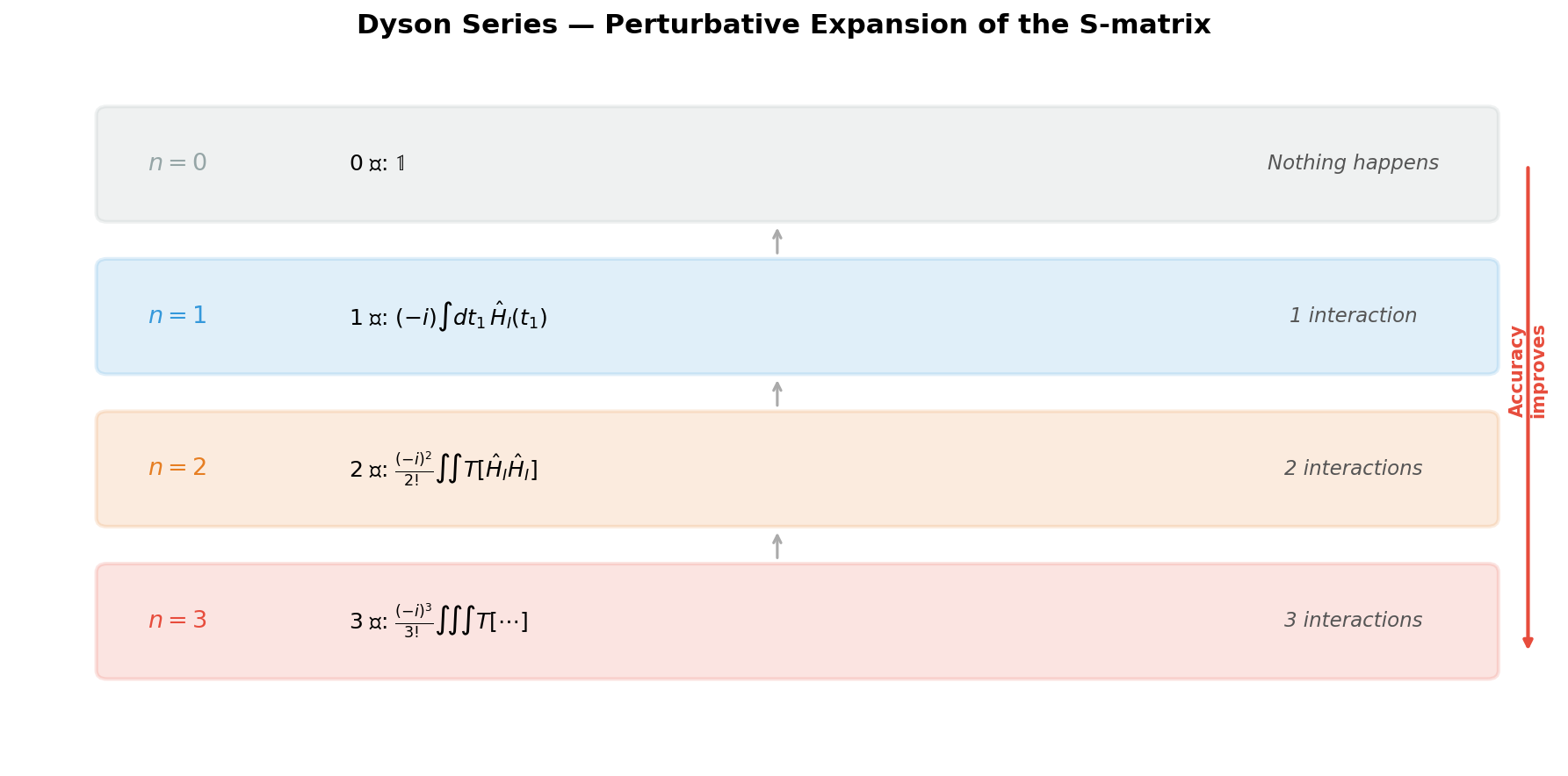
Fig. 7.3: The Dyson series — perturbative expansion of the S-matrix. The \(n\)-th order term corresponds to processes where the interaction occurs \(n\) times, with coefficient \((-i)^n/n!\) and time-ordered product \(T\) in each term. Higher orders improve accuracy.
🟡 Lina: And the S-operator is obtained by taking the limits \(t_0 \to -\infty\), \(t \to +\infty\):
In Lorentz-invariant form, using \(\hat{H}_I(t) = -\int d^3x\, \mathcal{L}_{\text{int}}(\hat{\phi}_I(x))\):
so
⚪ Mei: Equation (7.18) is a 4-dimensional integral, with \(\mathcal{L}_{\text{int}}\) being a scalar and \(d^4x\) a Lorentz-invariant measure, so the whole thing is in Lorentz-invariant form.
✅ Comprehension Check: Explain from the properties of the time-ordered product why the \(n\)-th order term in the Dyson series has the factor \(1/n!\).
Answer
When integrating the \(n\) time variables \(t_1, \ldots, t_n\) over the full region \([t_0, t]^n\), the time-ordered product ensures that all \(n!\) orderings give the same value. Therefore the integral over the full region is \(n!\) times the integral over the restricted region (\(t_1 > t_2 > \cdots > t_n\)). Since iterative substitution gives the integral over the restricted region, when extending to the full region we must divide by \(n!\).
7.5 Wick's Theorem — Decomposing Time-Ordered Products into "Contractions"
🟡 Lina: In each term of the Dyson series, time-ordered products of field operators appear. For example, at the lowest order (\(n=1\)) of \(\phi^4\) theory, we need to compute things like
But since each field operator is a sum of creation and annihilation operators, expanding directly produces an enormous number of terms. The tool for systematically organizing this is Wick's theorem.
Review of Normal Ordering \(:\!:\)
🟡 Lina: First, recall the normal ordering \(:\!\hat{A}\hat{B}\!:\). We introduced this operation in Ch. 4 to solve the vacuum energy problem. "Place all creation operators \(\hat{a}^\dagger\) to the left and all annihilation operators \(\hat{a}\) to the right" — for example, \(:\!\hat{a}_k \hat{a}_{k'}^\dagger\!: \;= \hat{a}_{k'}^\dagger \hat{a}_k\), just reordering (no sign change for bosons).
The important property of normal ordering is
because either the rightmost is always an annihilation operator so \(\hat{a}|0\rangle = 0\) kills the vacuum from the right, or the leftmost is always a creation operator so \(\langle 0|\hat{a}^\dagger = 0\) kills the vacuum from the left — one of these always happens.
🔵 Kai: The vacuum expectation value of a normal-ordered product is zero. Simple.
Definition of Contraction
🟡 Lina: Next, let me define the contraction of two field operators. It's defined as the "difference" between the time-ordered product and the normal-ordered product.
🔵 Kai: The time-ordered product minus the normal-ordered product...? What does that become?
🟡 Lina: Take the vacuum expectation value of both sides. From equation (7.19), the vacuum expectation value of the normal-ordered product is zero, so
The right-hand side is — the Feynman propagator \(D_F(x - y)\) that we computed in Ch. 4. So far this only says "the vacuum expectation value equals \(D_F\)," but in fact the contraction itself is not an operator but just a c-number (ordinary number), equal to \(D_F(x-y)\). I'll show why just below, but let me write the conclusion first.
In momentum space:
⚪ Mei: I see, taking the vacuum expectation value of the contraction kills the normal-ordered product, leaving only the vacuum expectation value of the time-ordered product — which is the propagator we saw in Chapter 4.
🔵 Kai: Oh! Contraction = Feynman propagator. That's easy to remember. But why does the contraction become just a "number" rather than an operator? It's a difference of field operators.
🟡 Lina: Good question. Let's split the field into positive and negative frequency parts.
Looking at the mode expansion (7.4), there are two types of terms: those with \(e^{-ip\cdot x}\) (containing \(\hat{a}\)) and those with \(e^{+ip\cdot x}\) (containing \(\hat{a}^\dagger\)). We call the former \(\hat{\phi}^+(x)\) and the latter \(\hat{\phi}^-(x)\). Specifically:
This is the same notation as when we split the photon field into \(A^{\mu(+)}\) (positive frequency part containing annihilation operators) and \(A^{\mu(-)}\) (negative frequency part containing creation operators) in Ch. 6. The notation might seem counterintuitive, so let me organize the mnemonics.
| Symbol | Contains | Plane wave form | Origin of name |
|---|---|---|---|
| \(\hat{\phi}^+(x)\) | Annihilation \(\hat{a}\) | \(e^{-i\omega t}\) (positive frequency) | Positive frequency part |
| \(\hat{\phi}^-(x)\) | Creation \(\hat{a}^\dagger\) | \(e^{+i\omega t}\) (negative frequency) | Negative frequency part |
So "\(+/-\) refers not to creation/annihilation but to the sign of \(E\) when writing the plane wave as \(e^{-iEt}\)" — \(e^{-i\omega t}\) is a wave with positive energy \(E = \omega > 0\) hence \(\hat{\phi}^+\), while \(e^{+i\omega t}\) is formally a negative energy wave hence \(\hat{\phi}^-\). This decomposition will also be used in the "matrix element calculation" later.
🔵 Kai: I see, "\(+\) is annihilation and \(-\) is creation" is hard to remember, but thinking of it as "the sign in the exponent of \(e\)" makes it make sense.
🟡 Lina: Right. Let's look concretely at the case \(t_1 > t_2\). By definition, the time-ordered product is \(T[\hat{\phi}(x_1)\hat{\phi}(x_2)] = \hat{\phi}(x_1)\hat{\phi}(x_2)\), which expands to
On the other hand, normal ordering moves all creation operators (\(\hat{\phi}^-\)) to the left, so looking at each term: - \(\hat{\phi}^+_1\hat{\phi}^+_2\): annihilation × annihilation → stays as is - \(\hat{\phi}^+_1\hat{\phi}^-_2\): annihilation × creation → move creation to left: \(\hat{\phi}^-_2\hat{\phi}^+_1\) - \(\hat{\phi}^-_1\hat{\phi}^+_2\): creation × annihilation → creation already on left → stays as is - \(\hat{\phi}^-_1\hat{\phi}^-_2\): creation × creation → stays as is
Therefore
Taking the difference, only the second term changed:
⚪ Mei: So the difference reduces to the commutator \([\hat{\phi}^+(x_1), \hat{\phi}^-(x_2)]\). And the reason this is a c-number is...
🟡 Lina: Right, recall that the free field commutation relation \([\hat{a}_k, \hat{a}_{k'}^\dagger] = (2\pi)^3\delta^{(3)}(\mathbf{k} - \mathbf{k}')\) is a delta function (a number) (Ch. 4). \([\hat{\phi}^+(x_1), \hat{\phi}^-(x_2)]\) is this commutation relation integrated over momentum, so the result is also a c-number. The case \(t_2 > t_1\) similarly gives \([\hat{\phi}^+(x_2), \hat{\phi}^-(x_1)]\), and combining both cases gives the Feynman propagator \(D_F(x_1 - x_2)\). That is, \(D_F(x-y) = \theta(x^0-y^0)[\hat{\phi}^+(x), \hat{\phi}^-(y)] + \theta(y^0-x^0)[\hat{\phi}^+(y), \hat{\phi}^-(x)]\). Here \(\theta\) is the step function, selecting which commutator to use depending on the time ordering.
⚪ Mei: I see, since the commutation relation itself is a c-number, integrating it still gives a c-number — so the contraction is not an operator but the "number" called the Feynman propagator. And the \(\theta\) function (step function, equal to 1 when the argument is positive and 0 when negative) precisely represents the "case distinction" of the time-ordered product.
✅ Comprehension Check: Why is a "contraction" of two field operators a c-number (ordinary number) rather than an operator?
Answer
The contraction is defined as the difference between the time-ordered product and the normal-ordered product. Splitting the field as \(\hat{\phi} = \hat{\phi}^+ + \hat{\phi}^-\), this difference reduces to the commutator of creation and annihilation operators \([\hat{\phi}^+(x), \hat{\phi}^-(y)]\). Since the free field commutation relation \([\hat{a}_k, \hat{a}_{k'}^\dagger] = (2\pi)^3\delta^{(3)}(\mathbf{k}-\mathbf{k}')\) is a delta function (a number), the contraction is also a c-number, equal to the Feynman propagator \(D_F(x-y)\).
Statement of Wick's Theorem
🟡 Lina: Now let me state Wick's theorem.
Wick's Theorem: The time-ordered product of field operators equals the normal-ordered product plus the sum of all possible contractions.
In formula, the time-ordered product of \(n\) fields is
🔵 Kai: What does "all possible contractions" mean concretely?
🟡 Lina: Let me show you explicitly with four fields. Below, I'll abbreviate \(\hat{\phi}_i \equiv \hat{\phi}(x_i)\). First look at the equation, then I'll explain how to read it.
Table 7.3: Structure of the 4-field expansion in Wick's theorem
| Number of contractions | Number of terms | Structure | Vacuum expectation value |
|---|---|---|---|
| 0 | 1 | \(:\!\hat{\phi}_1\hat{\phi}_2\hat{\phi}_3\hat{\phi}_4\!:\) | 0 |
| 1 | \(\binom{4}{2} = 6\) | \(D_F \times :\!\hat{\phi}\hat{\phi}\!:\) | 0 |
| 2 (full contraction) | 3 | \(D_F \times D_F\) (c-number) | Survives |
⚪ Mei: To organize: - Line 1: No contractions (the normal-ordered product itself) - Lines 2–3: One contraction (\(\binom{4}{2} = 6\) ways). Uncontracted fields remain inside normal ordering - Line 4: Two contractions (3 ways). All fields are contracted, no operators remain
🟡 Lina: And most importantly, when taking the vacuum expectation value, only the fully contracted terms (complete contractions) survive.
🔵 Kai: Since the vacuum expectation value of normal-ordered products is zero, all incomplete contraction terms vanish too! Only products of propagators remain.
🟡 Lina: This is the power of Wick's theorem. Complex products of operators reduce to products of Feynman propagators — which are just "numbers." The 3 terms in equation (7.25) correspond to the pairings "(1,2)(3,4)," "(1,3)(2,4)," and "(1,4)(2,3)" respectively. Check this visually in Fig. 7.4 "Contraction patterns in Wick's theorem for 4 fields".
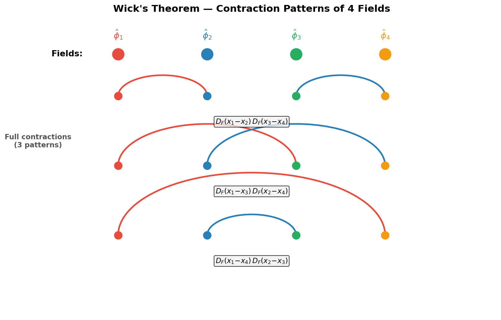
Fig. 7.4: Contraction patterns in Wick's theorem for 4 fields. There are 3 complete contractions of 4 fields. In the vacuum expectation value, only complete contractions survive, reducing to products of Feynman propagators.
✅ Comprehension Check: How many complete contractions contribute to the vacuum expectation value of the time-ordered product of 6 fields \(\hat{\phi}(x_1)\cdots\hat{\phi}(x_6)\)?
Answer
The number of ways to partition 6 fields into 3 pairs. The first field can be paired with 5 others, the next with 3, and the last with 1. So \(5 \times 3 \times 1 = 15\) ways. In general, for \(2n\) fields there are \((2n-1)!! = (2n-1)(2n-3)\cdots 3 \cdot 1\) ways.
📝 Exercises:
- Inductive derivation of Wick's theorem for 4 fields → Problem M-4. Normal Ordering and Wick's Theorem (Two-Field Case)
7.6 2→2 Scattering in \(\phi^4\) Theory — Lowest-Order Calculation
🟡 Lina: Using all the tools we've developed, let's finally calculate a concrete scattering amplitude. In \(\phi^4\) theory, let's find the lowest-order amplitude for the 2-particle scattering process
First-Order Term of the S-Matrix
🟡 Lina: The interaction Lagrangian density of \(\phi^4\) theory is \(\mathcal{L}_{\text{int}} = -\frac{\lambda}{4!}\phi^4\). Using the Lorentz-invariant form of the Dyson series (7.18), the first-order term is \(\hat{S}^{(1)} = i\int d^4x\, \mathcal{L}_{\text{int}}\), so
(Starting from the Hamiltonian form (7.17) gives the same result. Since \(\hat{H}_I(t) = -\int d^3x\,\mathcal{L}_{\text{int}}(\hat{\phi}_I) = +\frac{\lambda}{4!}\int d^3x\,\hat{\phi}_I^4\), we get \(-i\int dt\,\hat{H}_I(t) = -\frac{i\lambda}{4!}\int d^4x\,\hat{\phi}_I^4\), which matches)
(The first-order term of the Dyson series (7.18) originally has \(T\) applied, but here all four fields are at the same spacetime point \(x\). Bosonic fields at the same time and point commute with each other, so rearranging with \(T\) doesn't change the result — it can be omitted. Note that products of fields at the same point involve subtle operator ordering issues, but these don't affect tree-level calculations like ours)
🔵 Kai: This is the contribution where "the interaction happens just once."
🟡 Lina: Right. The scattering amplitude is
Calculating the Matrix Element
🟡 Lina: We need to substitute the mode expansion (7.4) of the field operator \(\hat{\phi}_I(x)\) and pick out the "2 annihilations + 2 creations" terms from \(\hat{\phi}_I(x)^4\).
🔵 Kai: Expanding everything looks like it'll be terrible...
🟡 Lina: But thanks to Wick's theorem, we can do it systematically. However, since this time we have external lines (particles in the initial and final states), let's be a bit more careful.
We split \(\hat{\phi}_I(x)\) into the positive frequency part \(\hat{\phi}^+(x)\) (containing annihilation operators \(\hat{a}_k\) and \(e^{-ik\cdot x}\)) and the negative frequency part \(\hat{\phi}^-(x)\) (containing creation operators \(\hat{a}_k^\dagger\) and \(e^{+ik\cdot x}\)), as introduced in "Definition of Contraction".
\(\hat{\phi}^+(x)\) "absorbs" particles from the initial state, and \(\hat{\phi}^-(x)\) "emits" particles into the final state. When expanding \(\hat{\phi}^4 = (\hat{\phi}^+ + \hat{\phi}^-)^4\), the terms that annihilate 2 incoming particles and create 2 scattered particles have the form \((\hat{\phi}^-)^2 (\hat{\phi}^+)^2\).
🔵 Kai: Choosing 2 for annihilation and 2 for creation out of 4 fields... how many ways are there?
🟡 Lina: The number of ways to choose 2 out of 4 for \(\hat{\phi}^+\) (annihilation) is \(\binom{4}{2} = 6\). Furthermore, among the chosen 2 \(\hat{\phi}^+\)'s, "which one absorbs \(p_1\) and which absorbs \(p_2\)" gives \(2! = 2\) ways. Similarly, among the 2 \(\hat{\phi}^-\)'s, "which one emits \(p_3\) and which emits \(p_4\)" gives \(2! = 2\) ways. In total: \(\binom{4}{2} \times 2! \times 2! = 6 \times 2 \times 2 = 24 = 4!\) ways.
⚪ Mei: \(4!\) ways — so it exactly cancels with the \(4!\) in the denominator.
🔵 Kai: Ah, \(4!\) appeared! It exactly cancels with the \(4!\) in the denominator!
🟡 Lina: Exactly! This is the reason for putting in the \(1/4!\) at the start.
🟡 Lina: Now, before calculating the matrix element of equation (7.27), let me organize the state normalization. In Chapter 4 we used the normalization \(|\mathbf{p}\rangle = \hat{a}_{\mathbf{p}}^\dagger|0\rangle\), but with this, \(\sqrt{2\omega}\) factors remain everywhere in scattering amplitude calculations, making things messy. Furthermore, when computing in different inertial frames (after Lorentz transformations), the form of the equations changes — inconvenient for a relativistic theory. So for scattering problems, it's standard to use covariant normalization (Lorentz-invariant normalization). We define states as
(Here, when writing \(|p\rangle\), the \(p\) denotes a 4-momentum, but the creation operator label is 3-momentum \(\mathbf{p}\). Since the mass-shell condition \(p^0 = \omega_{\mathbf{p}}\) determines the 4-momentum, \(|p\rangle\) and \(|\mathbf{p}\rangle\) refer to the same state.)
🔵 Kai: Multiplying by \(\sqrt{2\omega_p}\) on purpose must be because it gives some advantage, right?
🟡 Lina: Yes. Let me explain why \(\sqrt{2\omega_p}\) with two reasons in order. First, just stating the conclusion: with this choice, the inner product takes a Lorentz-invariant form. Let's actually compute it. Using the convention (7.4a) \([\hat{a}_{\mathbf{p}},\, \hat{a}_{\mathbf{q}}^\dagger] = (2\pi)^3\delta^{(3)}(\mathbf{p}-\mathbf{q})\):
(The \(\delta^{(3)}\) forces \(\mathbf{p} = \mathbf{q}\), so \(\omega_q = \omega_p\).)
This form is the same regardless of which inertial frame you compute in. From here on in this chapter, when I write \(|p\rangle\) without comment, it means covariant normalization. To summarize the notation change: compared to Chapter 4's \(|\mathbf{p}\rangle = \hat{a}_{\mathbf{p}}^\dagger|0\rangle\), from this chapter onward we use \(|p\rangle = \sqrt{2\omega_p}\,\hat{a}_p^\dagger|0\rangle\) — the only difference is the \(\sqrt{2\omega_p}\) factor.
🔵 Kai: Why is covariant normalization convenient?
🟡 Lina: There are two reasons.
First, the physical reason — this is somewhat advanced, so for now just hear it as "this is the motivation." With ordinary normalization \(\langle p|q\rangle = (2\pi)^3\delta^{(3)}(\mathbf{p}-\mathbf{q})\), the form of the inner product changes under Lorentz transformations (changing inertial frames). The reason is that in relativity, the mass-shell condition \(E = \omega_p = \sqrt{|\mathbf{p}|^2 + m^2}\) makes \(E\) and \(\mathbf{p}\) not independent, so under Lorentz transformations the 3-dimensional momentum space "volume element" \(d^3p\) itself changes.
🔵 Kai: What? \(d^3p\) changes? Even though it's just changing integration variables?
🟡 Lina: For example, consider a small box of width \(\Delta p_x\) in the \(p_x\) direction in one inertial frame. When you boost to another frame, \(E\) and \(p_x\) mix, so the same collection of particles occupies a different \(\Delta p_x'\) — because the mass-shell condition ties \(E\) to \(\mathbf{p}\), the volume in \(\mathbf{p}\)-space alone changes. It's similar to how changing map projections distorts areas. Specifically, it can be shown that only the combination \(d^3p/(2\omega_p)\) is Lorentz-invariant (we'll prove this in Ch. 8).
⚪ Mei: The delta function \(\delta^{(3)}(\mathbf{p}-\mathbf{q})\) satisfies \(\int d^3p\,\delta^{(3)} = 1\), so it has an "inverse" relationship with \(d^3p\) — meaning if \(d^3p/(2\omega_p)\) is invariant, then \(2\omega_p \cdot \delta^{(3)}\) is also an invariant combination.
🟡 Lina: Exactly. So by normalizing states with a factor of \(\sqrt{2\omega_p}\), the inner product automatically takes a Lorentz-invariant form — remember "in a relativistic theory, attaching \(\sqrt{2\omega_p}\) is natural."
🔵 Kai: I see, it's a convention for consistency with relativity.
🟡 Lina: Right. Next, the computational reason — this one we can verify concretely. Let's apply an annihilation operator to a covariantly normalized state. Using the commutation relation (7.4a) \([\hat{a}_k, \hat{a}_p^\dagger] = (2\pi)^3\delta^{(3)}(\mathbf{k}-\mathbf{p})\) and \(\hat{a}_k|0\rangle = 0\):
producing \(\sqrt{2\omega_p}\) and \((2\pi)^3\). Meanwhile, \(\hat{\phi}^+(x)\) from the mode expansion (7.4) contains \(1/[(2\pi)^3\sqrt{2\omega_k}]\). Applying \(\hat{\phi}^+(x)\) to \(|p\rangle_{\text{cov}}\): $$ \hat{\phi}^+(x)|p\rangle_{\text{cov}} = \int \frac{d^3k}{(2\pi)^3}\frac{1}{\sqrt{2\omega_k}}\, e^{-ik\cdot x}\, \hat{a}k|p\rangle|0\rangle $$}} = \int \frac{d^3k}{(2\pi)^3}\frac{\sqrt{2\omega_p}(2\pi)^3}{\sqrt{2\omega_k}}\, e^{-ik\cdot x}\,\delta^{(3)}(\mathbf{k}-\mathbf{p})|0\rangle = e^{-ip\cdot x
🔵 Kai: Wow, it cancels cleanly! Both \(\sqrt{2\omega}\) and \((2\pi)^3\) completely cancel out, leaving just the phase \(e^{-ip\cdot x}\).
🟡 Lina: Right. When the \(\delta^{(3)}\) fixes \(k = p\), we get \(\sqrt{2\omega_p}/\sqrt{2\omega_k} = 1\), and the \((2\pi)^3\) cancels with the denominator, cleanly leaving just the phase factor \(e^{-ip\cdot x}\). Similarly, \({}_{{\text{cov}}}\langle p_3|\hat{\phi}^-(x) = \langle 0|\, e^{ip_3\cdot x}\). Since this cancellation happens for each of the four fields, the matrix element — combining the \(4! = 24\) combinations we counted earlier — is
leaving only phase factors with all normalization factors cancelled. (The equality holds here because terms in the expansion of \(\hat{\phi}^4\) other than "exactly 2 annihilations + 2 creations" — such as terms where all 4 annihilate — give zero when sandwiched between \(\langle p_3, p_4|\) and \(|p_1, p_2\rangle\) because the particle numbers don't match)
⚪ Mei: So with covariant normalization, the pesky \(\sqrt{2\omega}\) factors automatically cancel and the calculation becomes clean.
Emergence of 4-Momentum Conservation
🟡 Lina: Substituting this into equation (7.27) and performing the \(d^4x\) integration:
So equation (7.27) becomes \(-\frac{i\lambda}{4!} \times 4! \times (2\pi)^4\delta^{(4)}(p_1+p_2-p_3-p_4) = -i\lambda\,(2\pi)^4\delta^{(4)}(p_1+p_2-p_3-p_4)\). The \(1/4!\) and the combinatorial factor \(4!\) neatly cancel.
🔵 Kai: A delta function appeared! This is...
🟡 Lina: 4-momentum conservation. Both energy and momentum are conserved. Because the interaction occurs locally at each spacetime point — meaning \(\mathcal{L}_{\text{int}}\) doesn't depend explicitly on the spacetime coordinate \(x\) — integrating \(e^{i(\Delta p)\cdot x}\) over all spacetime produces a delta function. The spatial integration \(\int d^3x\, e^{i\Delta\mathbf{p}\cdot\mathbf{x}}\) generates 3-dimensional momentum conservation, and the time integration \(\int dt\, e^{i\Delta E\, t}\) generates energy conservation.
⚪ Mei: So Noether's theorem — translational symmetry of spacetime leads to momentum conservation — appears concretely as a delta function in the scattering amplitude.
🟡 Lina: Precisely. This is an example of Noether's theorem — which we learned in Ch. 3, where translational symmetry of spacetime leads to momentum conservation — taking concrete effect in scattering amplitude calculations. The 4 components of \(\delta^{(4)}\) correspond one-to-one with translational symmetry in the 4 spacetime directions, and the symmetry of the theory directly connects to experimentally measurable scattering amplitudes. In other words, consequences of symmetry appear not only as conserved quantities but also as rules that select "allowed scattering processes." Conversely, if there were an external potential breaking spatial homogeneity, the corresponding delta function would disappear and momentum would not be conserved.
🔵 Kai: I see, so the flow symmetry → conservation law → delta function is directly visible in the calculation result.
✅ Comprehension Check: The appearance of the 4-momentum conservation delta function \(\delta^{(4)}(p_1+p_2-p_3-p_4)\) in the scattering amplitude calculation is the result of what mathematical operation?
Answer
Because the interaction occurs locally at each spacetime point, the phase factor \(e^{i(p_3+p_4-p_1-p_2)\cdot x}\) is integrated over all spacetime with \(d^4x\). This integral gives \((2\pi)^4\delta^{(4)}(p_1+p_2-p_3-p_4)\), and 4-momentum conservation naturally emerges.
Final Result: The Scattering Amplitude
🟡 Lina: Putting it all together, thanks to covariant normalization all \(\sqrt{2\omega}\) factors cancel, and substituting \(4! \times (2\pi)^4\delta^{(4)}\) into equation (7.27) with the \(1/4!\) cancellation, the S-matrix element is
Using the decomposition \(\hat{S} = \mathbb{1} + i\hat{T}\) from equation (7.12), we factor out the momentum-conserving delta function from the matrix elements of \(\hat{T}\) to define the invariant amplitude \(\mathcal{M}\).
In equation (7.29), we're considering a scattering process where initial and final states are different (\((p_1, p_2) \neq (p_3, p_4)\)), so \(\langle f|\mathbb{1}|i\rangle = 0\), and we can write \(\langle f|\hat{S}^{(1)}|i\rangle = \langle f|i\hat{T}^{(1)}|i\rangle\). Comparing:
🔵 Kai: What!? The result is this simple!? The scattering amplitude is just a constant \(-\lambda\)? But that means particles scatter with equal probability regardless of angle. Is that how it works in real scattering experiments?
🟡 Lina: At lowest order in \(\phi^4\) theory, yes. It depends neither on momentum nor on angle — isotropic scattering. This is because the \(\phi^4\) vertex just couples four fields "at a point," and no internal propagator appears. Incidentally, \(\phi^4\) theory itself doesn't directly describe real elementary particles — it's a "toy model" for learning the structure of quantum field theory. In real electron scattering (QED), the photon propagator enters, so even at lowest order there's angular dependence. In other words, whether angular dependence appears at lowest order is determined by "whether or not there are internal lines." We'll see that in Ch. 8 and beyond.
⚪ Mei: I see, \(\phi^4\) completes with a single vertex so there's no internal line and it's the constant \(-\lambda\). In QED internal lines come in and angles matter — looking forward to the next chapters.
🔵 Kai: With such a simple result, the next order is probably much more complicated... Ah, but wait. At the next order, propagators enter internally and you get angular dependence, right? But then, when integrating over internal momenta, it seems like something might diverge... is that okay?
🟡 Lina: Good intuition. At the next order and beyond, ultraviolet divergences (integrals becoming infinite) actually do occur when integrating over internal momenta. The systematic method for handling this is renormalization, which we'll treat properly in a later chapter. For now, remember that "divergences occur, but there exists a prescription to extract physically meaningful finite answers."
🟡 Lina: Now, if we draw the result we obtained as a diagram, it becomes a "×"-shaped diagram where 4 external lines meet at a single point (Fig. 7.5 "Lowest-order 2-body scattering vertex in φ⁴ theory"). This is one of the simplest Feynman diagrams. In the next chapter, Ch. 8, we'll systematically construct the correspondence rules between "pictures" and "formulas" — the Feynman rules.
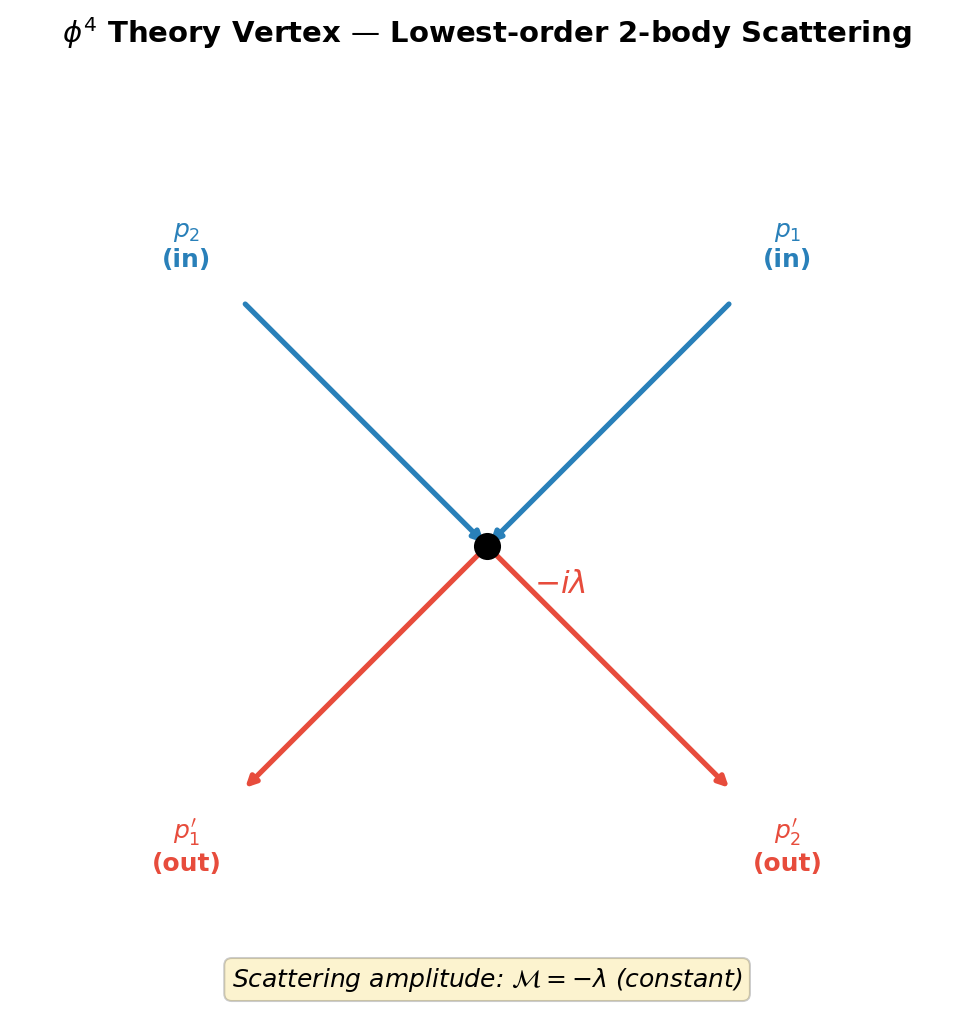
Fig. 7.5: Lowest-order 2-body scattering vertex in φ⁴ theory. The lowest-order diagram in \(\phi^4\) theory. Four external lines meet at a single point, and the scattering amplitude is the constant \(\mathcal{M} = -\lambda\).
✅ Comprehension Check: Physically explain why the lowest-order amplitude \(\mathcal{M} = -\lambda\) in 2→2 scattering in \(\phi^4\) theory does not depend on momentum.
Answer
At lowest order, the interaction occurs just once at a single spacetime point (one vertex). Since there is no virtual particle propagating internally, no propagator \(i/(p^2 - m^2 + i\varepsilon)\) appears, and no dependence on momentum transfer arises. Only the coupling constant \(\lambda\) determines the amplitude.
📝 Exercises:
- Lowest-order 2→2 amplitude in \(\phi^3\) theory and the Feynman propagator → Problem B-3. Explicit Calculation of the Time-Ordered Product
- Counting second-order diagrams for 2→2 scattering in \(\phi^4\) theory → Problem M-3. 2→2 Scattering Amplitude in \(\phi^4\) Theory (Leading Order)
7.7 Summary of This Chapter
🟡 Lina: Let's review today's content.
- Need for interactions: In free fields, particle number is conserved and neither scattering nor decay occurs. Real physics can only be described by adding \(\mathcal{L}_{\text{int}}\).
- Interaction picture: Operators evolve with \(\hat{H}_0\) (as free fields), and states evolve with \(\hat{H}_I(t)\). The tools of free field theory can be used as-is.
- S-matrix and Dyson series: All scattering information is encapsulated in \(\hat{S} = T\exp\!\left[i\int d^4x\, \mathcal{L}_{\text{int}}\right]\) (Lorentz-invariant form). Expanding this in powers of the coupling constant (Dyson series) allows systematic calculation of scattering amplitudes.
- Wick's theorem: Decomposes time-ordered products into normal-ordered products + contractions (= Feynman propagators). In vacuum expectation values, only complete contractions survive.
- 2→2 scattering in \(\phi^4\): At lowest order, \(\mathcal{M} = -\lambda\). 4-momentum conservation naturally emerges as a delta function.
🔵 Kai: We've finally entered the world where particles collide, leaving the world of free fields. I was moved by how Wick's theorem reduces those complex operator calculations to "combinatorics of pairings." But the number of pairings explodes as the number of fields increases, right? In the earlier check question, 6 fields gave 15 ways, and for 8 it'd be even more...
⚪ Mei: For 8 fields it's \(7 \times 5 \times 3 \times 1 = 105\) ways.
🔵 Kai: I knew it! At higher orders of the Dyson series the number of fields keeps growing, so writing everything out doesn't seem practical. How do you organize things in actual calculations?
🟡 Lina: The solution to precisely that problem is the Feynman diagrams we'll learn in the next chapter. By associating contraction patterns with "pictures," you can see at a glance which terms give physically equivalent contributions.
⚪ Mei: Controlling the combinatorial explosion through "classification by pictures." Looking forward to it.
Preview of Next Chapter
Ch. 8: Feynman Diagrams — Translating Pictures into Formulas
We visualize the contraction patterns obtained from Wick's theorem as "diagrams" and systematically construct the mathematical rules corresponding to vertices, internal lines, and external lines — the Feynman rules. We'll derive the Feynman rules for both \(\phi^4\) theory and QED, and experience the exhilaration of scattering amplitude calculations reducing to nothing more than "drawing pictures and translating."
References
- Quantum Field Theory for the Gifted Amateur (Lancaster & Blundell) Chapters 16–17 "Propagators and Green's functions / Propagators and fields" (background on Feynman propagators)
- Quantum Field Theory for the Gifted Amateur (Lancaster & Blundell) Chapter 18 "The S-matrix"
- Quantum Field Theory for the Gifted Amateur (Lancaster & Blundell) Chapter 19 "Expanding the S-matrix: Feynman diagrams"
- Quantum Field Theory (David Tong, Cambridge lecture notes) Chapter 3 "Interacting Fields"
- Quantum Field Theory and the Standard Model (Schwartz) Chapter 4 "Old-Fashioned Perturbation Theory"
- 坂本眞人『場の量子論 II — ファインマングラフとくりこみを中心にして』 Chapter 2 "Interacting fields and asymptotic fields"
- 坂本眞人『場の量子論 II — ファインマングラフとくりこみを中心にして』 Chapter 9 "Fluctuation expansion and Wick's theorem"
Feedback on this page
Let us know if something was unclear, incorrect, or could be improved.