Chapter 4: Quantization of Scalar Fields — Particles Born from Fields
Story so far:
In Ch. 3, we learned the Lagrangian formalism for classical fields and the Euler-Lagrange equations, and confirmed through Noether's theorem that continuous symmetries give rise to conserved quantities. We saw that the Klein-Gordon equation is derived from the Lagrangian density of a real scalar field, and that the Hamiltonian density describes the spatial distribution of energy.
Goals of this chapter
- Perform "canonical quantization" of the classical Klein-Gordon field and extract creation and annihilation operators from the Fourier expansion of the field
- Mathematically realize how field excitations naturally appear as "particles" as a result
- Furthermore, understand the mechanism by which antiparticles automatically emerge from the quantization of a complex scalar field, and confirm the Casimir effect as a physical consequence of zero-point energy
4.1 What Is Canonical Quantization? — Extending Quantum Mechanics to Fields
🟡 Lina: Now we're entering the heart of quantum field theory. Up through Ch. 3, we've been building up the Lagrangian formalism for classical fields. Today we'll "quantize" that classical field — that is, promote the field to an operator and extract quantum mechanical particles from it. I've summarized the overall flow in Fig. 4.1 "Flow of canonical quantization: from classical field to particles. The 4 steps", so let's first confirm the big picture. Starting from the Lagrangian, we find the conjugate momentum and Hamiltonian, impose equal-time commutation relations, and introduce creation and annihilation operators through Fourier expansion — in these 4 steps, field excitations appear as particles.
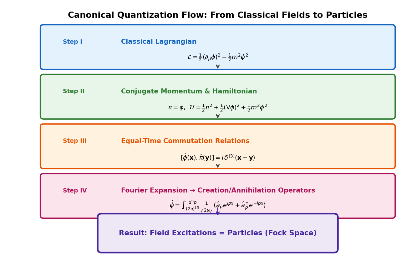
Fig. 4.1: Flow of canonical quantization: from classical field to particles. The 4 steps — Lagrangian → conjugate momentum & Hamiltonian → equal-time commutation relations → Fourier expansion & creation/annihilation operators — make field excitations appear as particles.
🔵 Kai: "Quantization" means doing the same thing to fields that we did in quantum mechanics when we imposed \([\hat{x}, \hat{p}] = i\)?
🟡 Lina: Exactly right. In quantum mechanics, we promoted classical coordinates \(q\) and momenta \(p\) to operators \(\hat{q}\), \(\hat{p}\) and imposed the commutation relation \([\hat{q}, \hat{p}] = i\). In field theory, we do exactly the same thing. However, in quantum mechanics the degrees of freedom were distinguished by discrete indices \(i\) like "the 1st spring, the 2nd spring, ..." but in field theory, each point \(\mathbf{x}\) in space carries its own independent degree of freedom — meaning the continuous coordinate \(\mathbf{x}\) becomes the label for degrees of freedom. In other words, field theory deals with infinitely many degrees of freedom.
⚪ Mei: The discrete index \(i\) gets replaced by the continuous coordinate \(\mathbf{x}\). An extension from finite to infinite.
🟡 Lina: Exactly. This procedure is called canonical quantization. Let me show you the overall flow first.
Table 4.1: Steps of canonical quantization
| Step | What to do |
|---|---|
| Step I | Write down the classical Lagrangian density \(\mathcal{L}\) |
| Step II | Find the conjugate momentum density \(\pi(x)\) and Hamiltonian density \(\mathcal{H}\) |
| Step III | Promote the field and momentum density to operators and impose equal-time commutation relations |
| Step IV | Fourier expand the field and introduce creation/annihilation operators |
Steps I and II were already done in Ch. 3, so today we'll start from Step III.
🔵 Kai: So we can use the results from Ch. 3. Let me recall — we found the conjugate momentum density and Hamiltonian density from the Lagrangian density, right?
🟡 Lina: Yes. Let me review. The Lagrangian density is
The conjugate momentum density is
🔵 Kai: The conjugate momentum being the time derivative of the field itself is thanks to the simplicity of the real scalar field, right?
🟡 Lina: That's right. The Hamiltonian density is
Now let's proceed to Step III.
✅ Comprehension Check: What do we do in Step III of canonical quantization? Describe the similarities and differences with canonical quantization in quantum mechanics.
Answer
In Step III, we promote the classical field \(\phi(x)\) and conjugate momentum density \(\pi(x)\) to operators and impose equal-time commutation relations. This is the same spirit as imposing \([\hat{q}_i, \hat{p}_j] = i\,\delta_{ij}\) in quantum mechanics, but since the label for degrees of freedom is a continuous spatial coordinate \(\mathbf{x}\) rather than a discrete index \(i\), the Kronecker delta is replaced by the Dirac delta function \(\delta^{(3)}(\mathbf{x} - \mathbf{y})\).
4.2 Equal-Time Commutation Relations — Promoting Fields to Operators
🟡 Lina: We will now promote the classical field \(\phi(x)\) and conjugate momentum density \(\pi(x)\) to operators. As we learned in Quantum Mechanics Ch. 5, an operator is a mathematical object that acts on a state vector and returns another state vector, and in general, swapping the order of multiplication changes the result (non-commutativity). The important point here is that the field operator \(\hat{\phi}(t, \mathbf{x})\) has one operator at each point \(\mathbf{x}\) in space. In quantum mechanics we had a finite number of operators \(\hat{q}_1, \hat{q}_2, \ldots\), but in field theory, an operator is "attached" to every point in space.
🔵 Kai: An operator placed at every point in space... that's an enormous number.
🟡 Lina: Yes, a continuous infinity. In the same spirit as imposing
in quantum mechanics, in field theory we impose the equal-time commutation relations.
🔵 Kai: The \(\delta_{ij}\) from quantum mechanics is replaced by \(\delta^{(3)}(\mathbf{x} - \mathbf{y})\). But why does the Dirac delta function appear?
🟡 Lina: Good question. In quantum mechanics, degrees of freedom were discrete, so the Kronecker delta \(\delta_{ij}\) was sufficient to express "1 if same degree of freedom, 0 if different." But in field theory, each point \(\mathbf{x}\) in space carries an independent degree of freedom. To express "nontrivial at the same point, zero at different points" for a continuous label, we need the Dirac delta function \(\delta^{(3)}(\mathbf{x} - \mathbf{y})\).
⚪ Mei: Summarizing Lina's explanation in a table, it looks like this.
Table 4.2: Correspondence between quantum mechanics and quantum field theory
| Quantum Mechanics (finite degrees of freedom) | Quantum Field Theory (infinite degrees of freedom) |
|---|---|
| Index \(i = 1, 2, \ldots, n\) | Spatial coordinate \(\mathbf{x}\) |
| \(\hat{q}_i(t)\) | \(\hat{\phi}(t, \mathbf{x})\) |
| \(\hat{p}_i(t)\) | \(\hat{\pi}(t, \mathbf{x})\) |
| \(\delta_{ij}\) | \(\delta^{(3)}(\mathbf{x} - \mathbf{y})\) |
🟡 Lina: Nice summary. Let me add one more row: the sum over discrete degrees of freedom \(\sum_i\) gets replaced by a spatial integral \(\int d^3x\) for continuous degrees of freedom. Same spirit as the delta function correspondence.
⚪ Mei: I see, \(\sum_i \to \int d^3x\) is also part of the correspondence. Also, equation (4.4) is called the "equal-time" commutation relation, meaning it holds only at the same time \(t\), right?
🟡 Lina: Exactly. Equation (4.4) holds only at the same time \(t\). That's why it's called the "equal-time" commutation relation. The commutation relations of fields at different times are determined separately through time evolution.
🔵 Kai: Treating time and space on equal footing is the spirit of relativity, but here we're singling out time as special, aren't we?
🟡 Lina: Sharp observation. In canonical quantization, we need to single out the time direction in order to use the Hamiltonian, so Lorentz invariance temporarily becomes less transparent. But don't worry — the final theory is properly Lorentz invariant. As an analogy, when drawing a map of the Earth, you need to "cut" somewhere to unfold the sphere onto a flat surface, but the Earth itself remains a sphere — it's a similar situation. We're choosing the time direction only as part of the calculation, and the physical laws themselves don't depend on the spacetime direction. Specifically, when we compute the commutation relations of fields at different times (Lorentz-invariant propagators) in Ch. 6, this will be confirmed.
🔵 Kai: The map analogy is very clear. We're choosing time as a "tool" for calculation, but the physical results don't depend on that choice. It feels a bit uncomfortable, but I'll move forward.
✅ Comprehension Check: In the equal-time commutation relation \([\hat{\phi}(t, \mathbf{x}), \hat{\pi}(t, \mathbf{y})] = i\,\delta^{(3)}(\mathbf{x} - \mathbf{y})\), what is the value of the commutator when \(\mathbf{x} \neq \mathbf{y}\)? What is its physical meaning?
Answer
When \(\mathbf{x} \neq \mathbf{y}\), \(\delta^{(3)}(\mathbf{x} - \mathbf{y}) = 0\), so the commutator is zero. This means the field and momentum density at different spatial points are independent degrees of freedom that can simultaneously have definite values. This reflects the "locality of field theory" — physical quantities at widely separated points do not interfere with each other.
4.3 Intuitive Picture — "Particles Are Excitations of Fields"
🟡 Lina: Before diving into the mathematical calculations, I want to share an intuitive picture of what we're trying to accomplish. The core idea of quantum field theory can be stated in one phrase — particles are excitations of fields.
🔵 Kai: "Excitation" means receiving energy and going to a higher state, right?
🟡 Lina: Exactly. Imagine a rubber sheet. The sheet stretched flat and still is the "vacuum." If you flick the sheet with your finger and one point vibrates, that's "one particle." If another point vibrates simultaneously, that's "two particles." In other words, particles are not independently existing "things" but rather states of the field itself. Particles appear as "localized fluctuations where the field is rippling above a quiet background."
⚪ Mei: So the identity of a particle is a local vibration of the field, and the quiet background sheet corresponds to the vacuum.
🟡 Lina: Exactly right. The beauty of this picture is:
Table 4.3: Rubber sheet picture of particles as field excitations
| Phenomenon | Rubber sheet picture |
|---|---|
| Vacuum | Sheet is at rest |
| One particle | Vibrating at one location |
| Two particles | Vibrating at two locations |
| Particle creation | A new vibration starts |
| Particle annihilation | Vibration subsides back to rest |
| Why identical particles are indistinguishable | Because every vibration is a ripple of the same sheet |
🔵 Kai: Processes where particle number changes can be naturally described as the sheet going between rest, vibration, and rest! In quantum mechanics, particle number was fixed, but in the field picture, creation and annihilation naturally enter!
🟡 Lina: Yes. And the greatest motivation for why quantum field theory is needed — non-conservation of particle number (see Chapter 1) — is built into the design from the start in this picture. Photons are excitations of the electromagnetic field, electrons are excitations of the electron field, quarks are excitations of the quark field — there are several fields in the universe, and particles appear as ripples of those fields. This is the worldview of quantum field theory.
✅ Comprehension Check: In the picture of "particles are excitations of fields," how are particle creation and annihilation understood?
Answer
A new vibration starting on top of a quiet state (vacuum) corresponds to "particle creation," and a vibration subsiding back to rest corresponds to "particle annihilation." Since particles are not independently existing "things" but states of the field itself, changes in particle number are naturally described as changes in the vibrational state of the field.
🟡 Lina: And there's another important perspective. In quantum mechanics, particles were assumed from the start — the "vibrating point" was the starting point. But in quantum field theory, "the sheet itself" is the starting point, and vibrations (= particles) emerge as a result of quantization. Particles are derived from a more fundamental object — the field. This makes the framework more fundamental. The starting point has gone one level deeper.
⚪ Mei: So in quantum mechanics, we wrote wave functions assuming "particles exist," but in quantum field theory, we only assume "fields exist," and both the existence of particles and changes in particle number are all derived from there. With one fewer assumption, the explanatory power increases.
🟡 Lina: Exactly. What we'll do in the following sections is realize this intuitive picture rigorously in equations. Specifically:
- Fourier expand the field \(\phi(x)\) to decompose it into "infinitely many independent vibrational modes"
- Quantize each mode as a harmonic oscillator to obtain creation and annihilation operators
- The creation operator \(\hat{a}_{\mathbf{p}}^\dagger\) "adds one vibration" = creates one particle
- Construct the Fock space containing multi-particle states
In the rubber sheet analogy, this is the procedure of "decomposing waves running on the sheet into a superposition of sine waves, and quantizing each wave." Let's now realize this in equations.
4.4 Fourier Expansion and Decomposition into Harmonic Oscillators
🟡 Lina: Now let's get our hands dirty. First, we Fourier expand the field.
🔵 Kai: A Fourier expansion means representing something as a superposition of waves, right? Why does this make calculations easier?
🟡 Lina: That's a question that hits the core. Recall the Klein-Gordon equation:
Writing this in components:
Now we Fourier transform the field only in the spatial directions. The purpose is to "decompose the partial differential equation into ordinary differential equations (equations in time only) for each mode." The spatial derivative \(\nabla^2\) gets replaced by an algebraic factor under Fourier transformation, but we want to keep the time derivative \(\ddot{\phi}\) as is — so we transform only in space and leave time alone.
⚪ Mei: We Fourier transform to "untangle" the partial differential equation into independent ordinary differential equations for each mode.
🟡 Lina: Right. A Fourier transform means representing the field as "a superposition of plane waves \(e^{i\mathbf{p}\cdot\mathbf{x}}\) of various wavelengths."
\(\tilde{\phi}(\mathbf{p}, t)\) is the Fourier coefficient representing "how much amplitude the plane wave corresponding to momentum \(\mathbf{p}\) contributes," and it's a function of time. The spatial derivative \(\nabla^2\) gets replaced by the algebraic factor \(-|\mathbf{p}|^2\) under Fourier transformation, but we want to keep the time derivative \(\ddot{\phi}\) as is — this way each mode becomes "a differential equation in time only" that can be treated as a harmonic oscillator. The reason we call the Fourier transform variable \(\mathbf{p}\) "momentum" comes from the de Broglie relation \(p = \hbar k\) in quantum mechanics. In natural units (\(\hbar = 1\)), the wave number \(k\) and momentum \(p\) have the same numerical value, so we can call the Fourier transform variable directly "momentum." The \((2\pi)^{3/2}\) in the denominator is a normalization factor. This is a convention ensuring "transforming and then inverse transforming returns the original," and the inverse transform is
We're using the convention where \((2\pi)^{3/2}\) enters equally in both the transform (4.8) and the inverse transform (4.8').
🔵 Kai: Why is this normalization consistent?
🟡 Lina: Let's check explicitly. Substitute the inverse transform formula into \(\phi(t, \mathbf{x})\) from equation (4.8) to eliminate \(\tilde{\phi}\). Then \(\frac{1}{(2\pi)^{3/2}} \times \frac{1}{(2\pi)^{3/2}} = \frac{1}{(2\pi)^3}\) appears in front of the \(\mathbf{x}'\) integral. The remaining \(\mathbf{x}'\) integral is
This is the 3-dimensional version of equation (C.30) from @chapter:qm/appendix_c. Since a delta function appears, the \(\mathbf{q}\) integral gets fixed to \(\mathbf{q} = \mathbf{p}\), recovering the original \(\tilde{\phi}(\mathbf{p})\). In short, the round trip of transform → inverse transform produces \((2\pi)^3\) in the denominator, which exactly matches the \((2\pi)^3\) in the integral representation of the delta function, so the original function is recovered — that's all there is to it. Some textbooks use a convention that puts all of \((2\pi)^3\) on one side, but the physical results are unaffected.
🔵 Kai: The Fourier coefficient \(\tilde{\phi}(\mathbf{p}, t)\) is generally complex, right? But \(\phi\) is a real scalar field so it should be real... isn't that a contradiction?
🟡 Lina: Good question. For a real scalar field, there's a condition \(\tilde{\phi}(-\mathbf{p}, t) = \tilde{\phi}(\mathbf{p}, t)^*\), which makes \(\phi(t, \mathbf{x})\) real overall (this will be important when we do the mode expansion later). To briefly see why this condition ensures reality: taking the complex conjugate of equation (4.8) gives \(\phi^* = \int \frac{d^3p}{(2\pi)^{3/2}} e^{-i\mathbf{p}\cdot\mathbf{x}} \tilde{\phi}(\mathbf{p})^*\), and substituting \(\mathbf{p} \to -\mathbf{p}\) gives \(\phi^* = \int \frac{d^3p}{(2\pi)^{3/2}} e^{i\mathbf{p}\cdot\mathbf{x}} \tilde{\phi}(-\mathbf{p})^*\). For \(\phi = \phi^*\) to hold, we need \(\tilde{\phi}(\mathbf{p}) = \tilde{\phi}(-\mathbf{p})^*\) — so reality and the condition on Fourier coefficients are equivalent. Substituting this into equation (4.7) —
⚪ Mei: Reality imposes a condition on the Fourier coefficients. Let's see what happens to the partial differential equation.
🟡 Lina: When \(\nabla^2\) acts on \(e^{i\mathbf{p}\cdot\mathbf{x}}\), it gives \(-|\mathbf{p}|^2\, e^{i\mathbf{p}\cdot\mathbf{x}}\) (check: \(\frac{\partial}{\partial x}e^{i p_x x} = i p_x\, e^{i p_x x}\), so differentiating twice gives \((i p_x)^2 = -p_x^2\). Same for \(y\) and \(z\) directions, totaling \(\nabla^2 e^{i\mathbf{p}\cdot\mathbf{x}} = -(p_x^2 + p_y^2 + p_z^2)\,e^{i\mathbf{p}\cdot\mathbf{x}} = -|\mathbf{p}|^2\,e^{i\mathbf{p}\cdot\mathbf{x}}\)). Substituting equation (4.8) into equation (4.7):
Since \(e^{i\mathbf{p}\cdot\mathbf{x}}\) are linearly independent for different \(\mathbf{p}\), the bracket must be zero for all \(\mathbf{p}\). (This is the same logic as "if \(a\sin x + b\sin 2x + \cdots = 0\) holds for all \(x\), then \(a = b = \cdots = 0\)" from the uniqueness of Fourier series. Specifically, multiplying both sides by \(e^{-i\mathbf{q}\cdot\mathbf{x}}\) and integrating over \(\mathbf{x}\), orthogonality leaves only the \(\mathbf{p} = \mathbf{q}\) term, showing the bracket is zero.) Therefore, for each \(\mathbf{p}\):
⚪ Mei: Each momentum mode satisfies an independent differential equation. And it's become a differential equation in \(t\) only.
🔵 Kai: This is the form \(\ddot{X} + \omega^2 X = 0\)! That's the harmonic oscillator equation of motion we studied extensively in quantum mechanics!
🟡 Lina: Exactly! This is the heart of quantum field theory. When you Fourier transform the Klein-Gordon field, it decomposes into infinitely many independent harmonic oscillators labeled by momentum \(\mathbf{p}\). The angular frequency of each oscillator is
which is exactly the relativistic energy-momentum relation \(E = \sqrt{p^2 + m^2}\).
⚪ Mei: So quantizing the field reduces to "quantizing infinitely many harmonic oscillators."
🟡 Lina: Exactly. And since we know how to quantize harmonic oscillators, we can directly use the creation and annihilation operators from Quantum Mechanics Ch. 12. Let's translate that technique into the language of fields. I've summarized the overall picture in Fig. 4.2 "Fourier mode decomposition of the Klein-Gordon field", so take a look.
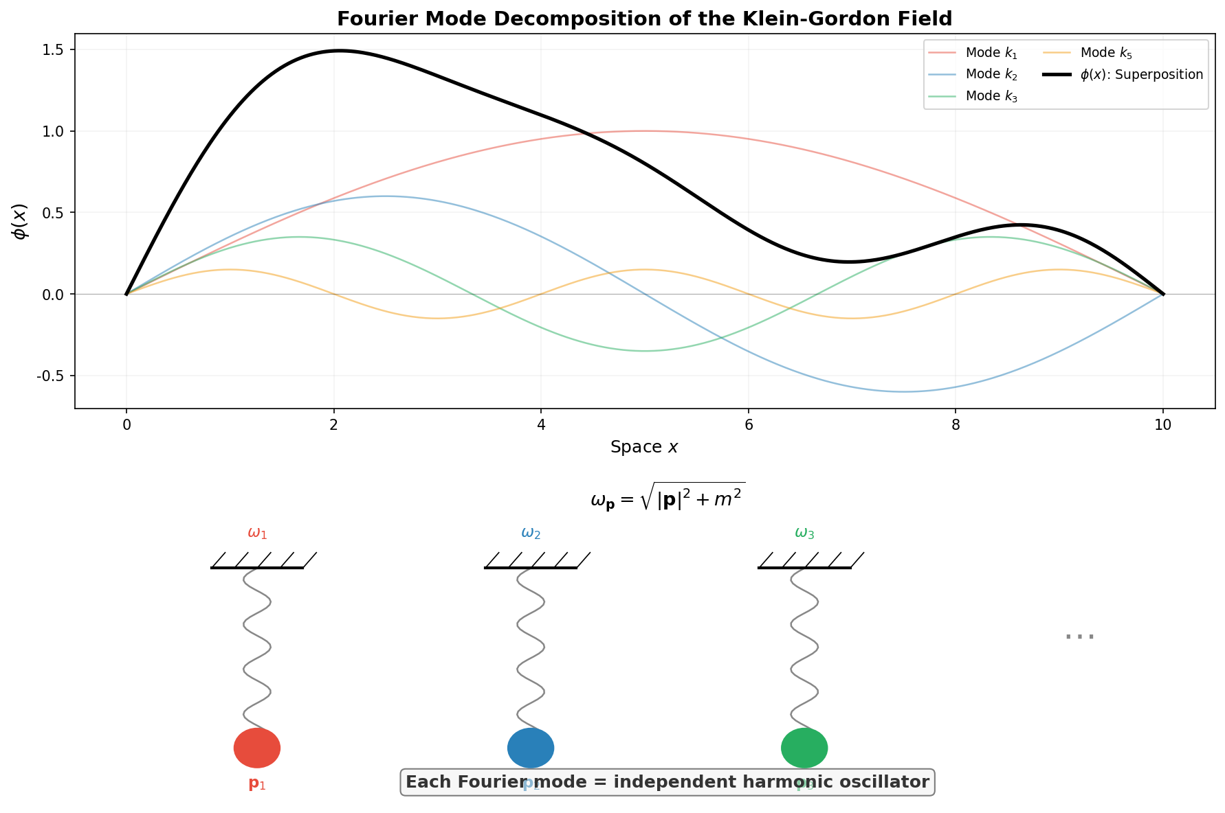
Fig. 4.2: Fourier mode decomposition of the Klein-Gordon field. Fourier expanding the Klein-Gordon field makes each momentum mode an independent harmonic oscillator. The frequency \(\omega_{\mathbf{p}} = \sqrt{|\mathbf{p}|^2 + m^2}\) is the relativistic energy-momentum relation itself.
✅ Comprehension Check: When the Klein-Gordon field is Fourier transformed in the spatial directions, what form of equation does the partial differential equation decompose into? Why is this important?
Answer
It decomposes into an independent ordinary differential equation \(\ddot{\tilde{\phi}} + \omega_{\mathbf{p}}^2 \tilde{\phi} = 0\) for each momentum mode \(\mathbf{p}\). This has the same form as the harmonic oscillator equation of motion, so the creation and annihilation operator techniques established in quantum mechanics can be applied directly, making systematic quantization of the field possible.
✅ Comprehension Check: When the Klein-Gordon field is Fourier transformed, how is the frequency \(\omega_{\mathbf{p}}\) of each mode expressed? What relation does this correspond to?
Answer
\(\omega_{\mathbf{p}} = \sqrt{|\mathbf{p}|^2 + m^2}\). This corresponds to the relativistic energy-momentum relation \(E^2 = p^2 + m^2\) (in natural units). That is, the frequency of each Fourier mode gives the energy of the particle corresponding to that mode.
4.5 Introducing Creation and Annihilation Operators — Mode Expansion of the Field
From Harmonic Oscillator Review to Field Theory
🟡 Lina: Do you remember how creation and annihilation operators were defined for the quantum mechanical harmonic oscillator?
🔵 Kai: Yes. For the Hamiltonian \(\hat{H} = \frac{1}{2}\hat{p}^2 + \frac{1}{2}\omega^2 \hat{q}^2\) (in natural units \(\hbar = 1\), with oscillator mass \(m = 1\)), the annihilation and creation operators are defined as
and the commutation relation \([\hat{a}, \hat{a}^\dagger] = 1\) holds, right?
🟡 Lina: That's right. Let me supplement why this formula can be used directly in field theory. Looking at equation (4.9), each Fourier mode \(\tilde{\phi}(\mathbf{p}, t)\) satisfies \(\ddot{\tilde{\phi}} + \omega_{\mathbf{p}}^2 \tilde{\phi} = 0\). The conjugate momentum is \(\tilde{\pi} = \dot{\tilde{\phi}}\). If we put the system in a finite box (volume \(V\)) to discretize the momenta, the right-hand side of the field's equal-time commutation relation (4.4), \(\delta^{(3)}(\mathbf{x}-\mathbf{y})\), gets replaced by \(V^{-1}\sum_{\mathbf{p}} e^{i\mathbf{p}\cdot(\mathbf{x}-\mathbf{y})}\). Fourier transforming this gives the commutation relation for each mode as \([\tilde{\phi}_{\mathbf{p}}, \tilde{\pi}_{\mathbf{q}}] = i\,\delta_{\mathbf{p}\mathbf{q}}\) — meaning it's zero between different modes and \(i\) for the same mode. This means each mode has the same structure as an independent harmonic oscillator with "mass 1, angular frequency \(\omega_{\mathbf{p}}\)." So the formulas above apply directly (in the continuous limit, \(\delta_{\mathbf{p}\mathbf{q}}\) returns to \(\delta^{(3)}(\mathbf{p}-\mathbf{q})\), but the operator definitions themselves take the same form as in the discrete case).
🔵 Kai: I see, since each Fourier mode has the same commutation relation as an independent harmonic oscillator, we can use the quantum mechanics formulas as they are.
🟡 Lina: Exactly. And solving inversely:
and the Hamiltonian becomes \(\hat{H} = \omega\left(\hat{a}^\dagger \hat{a} + \frac{1}{2}\right)\). Check it — expanding \(\hat{a}^\dagger \hat{a} = \left(\sqrt{\frac{\omega}{2}}\hat{q} - \frac{i}{\sqrt{2\omega}}\hat{p}\right)\left(\sqrt{\frac{\omega}{2}}\hat{q} + \frac{i}{\sqrt{2\omega}}\hat{p}\right)\) produces \(\hat{q}\hat{q}\) and \(\hat{p}\hat{p}\) terms plus cross terms \(\hat{q}\hat{p}\) and \(\hat{p}\hat{q}\). Specifically, \(\frac{\omega}{2}\hat{q}^2 + \frac{1}{2\omega}\hat{p}^2 + \frac{i}{2}(\hat{q}\hat{p} - \hat{p}\hat{q})\), where the last bracket is the commutator \([\hat{q}, \hat{p}] = i\) itself. Substituting gives \(\frac{\omega}{2}\hat{q}^2 + \frac{1}{2\omega}\hat{p}^2 - \frac{1}{2}\). Since \(\hat{H} = \frac{1}{2}\hat{p}^2 + \frac{1}{2}\omega^2\hat{q}^2\), we have \(\frac{\omega}{2}\hat{q}^2 + \frac{1}{2\omega}\hat{p}^2 = \frac{1}{\omega}\hat{H}\), so \(\hat{a}^\dagger \hat{a} = \frac{1}{\omega}\hat{H} - \frac{1}{2}\), yielding \(\hat{H} = \omega(\hat{a}^\dagger \hat{a} + \frac{1}{2})\). This was done in detail in Quantum Mechanics Ch. 9, so I'll just use the result here.
⚪ Mei: The form expressing \(q\) as a sum of \(a\) and \(a^\dagger\). I wonder if this will be used in the field mode expansion.
🟡 Lina: Exactly right. This inverted form — expressing \(q\) in terms of \(a\) and \(a^\dagger\) — directly connects to the form we'll use for the field mode expansion. The current Klein-Gordon field is a harmonic oscillator with angular frequency \(\omega_{\mathbf{p}}\) for each momentum \(\mathbf{p}\). So for each mode, we introduce an annihilation operator \(\hat{a}_{\mathbf{p}}\) and creation operator \(\hat{a}_{\mathbf{p}}^\dagger\).
Specifically, since the Fourier coefficient \(\tilde{\phi}(\mathbf{p}, t)\) in equation (4.8) corresponds to the "coordinate" of a harmonic oscillator with angular frequency \(\omega_{\mathbf{p}}\), we want to write it using the correspondence \(q = \frac{1}{\sqrt{2\omega}}(a + a^\dagger)\) that Kai reviewed. In the harmonic oscillator, we expressed \(q\) in terms of \(a\) and \(a^\dagger\). Similarly, assigning an annihilation operator \(\hat{a}_{\mathbf{p}}\) to each mode \(\mathbf{p}\):
The reason \(\hat{a}_{-\mathbf{p}}^\dagger\) enters is to satisfy the real scalar field condition. Classically, the reality condition was \(\tilde{\phi}(-\mathbf{p}) = \tilde{\phi}(\mathbf{p})^*\) (complex conjugate). After quantization and promotion to operators, complex conjugation \(*\) is replaced by Hermitian conjugation \(\dagger\). The reason is that classically "\(\phi\) is real" means \(\phi = \phi^*\), but in the operator world, "\(\hat{\phi}\) is real-valued (= returns real measurement values as an observable)" means \(\hat{\phi} = \hat{\phi}^\dagger\) — that is, Hermiticity. As we learned in Quantum Mechanics Ch. 8, eigenvalues of Hermitian operators are always real. Check: substituting \(\mathbf{p} \to -\mathbf{p}\) in this formula gives \(\tilde{\phi}(-\mathbf{p}) = \frac{1}{\sqrt{2\omega_{\mathbf{p}}}}(\hat{a}_{-\mathbf{p}} + \hat{a}_{\mathbf{p}}^\dagger)\). Meanwhile, the Hermitian conjugate of the original is \(\tilde{\phi}(\mathbf{p})^\dagger = \frac{1}{\sqrt{2\omega_{\mathbf{p}}}}(\hat{a}_{\mathbf{p}}^\dagger + \hat{a}_{-\mathbf{p}})\). Indeed \(\tilde{\phi}(-\mathbf{p}) = \tilde{\phi}(\mathbf{p})^\dagger\) holds.
🔵 Kai: I see, reality gets translated to Hermiticity, and that determines the necessity of \(\hat{a}_{-\mathbf{p}}^\dagger\).
🟡 Lina: Substituting this into equation (4.8) and rearranging: the \(\hat{a}_{\mathbf{p}}\) terms come with \(e^{i\mathbf{p}\cdot\mathbf{x}}\) directly. For the \(\hat{a}_{-\mathbf{p}}^\dagger\) terms, substituting the integration variable \(\mathbf{p} \to -\mathbf{p}\) (the integration range is \(-\infty\) to \(+\infty\) so it doesn't change), \(e^{i(-\mathbf{p})\cdot\mathbf{x}} = e^{-i\mathbf{p}\cdot\mathbf{x}}\) appears, and the operator becomes \(\hat{a}_{-(-\mathbf{p})}^\dagger = \hat{a}_{\mathbf{p}}^\dagger\). This gives us the mode expansion of the field operator. Let me first write the form at time \(t = 0\) (time evolution will be added shortly). The Fourier coefficient \(\tilde{\phi}(\mathbf{p}, t)\) in equation (4.8) is a function of time, but what we've expressed in terms of \(\hat{a}_{\mathbf{p}}\) and \(\hat{a}_{\mathbf{p}}^\dagger\) is its value at \(t = 0\). The argument is \(\hat{\phi}(\mathbf{x})\) with only the spatial coordinate because we've fixed \(t = 0\).
🔵 Kai: Let me check something. When we later compute the conjugate momentum \(\hat{\pi} = \dot{\hat{\phi}}\), what happens to the \(\frac{1}{\sqrt{2\omega_{\mathbf{p}}}}\) factor?
🟡 Lina: Good question. When we time-differentiate \(\hat{\phi}\), \(e^{-i\omega_{\mathbf{p}} t}\) produces \(-i\omega_{\mathbf{p}}\) and \(e^{+i\omega_{\mathbf{p}} t}\) produces \(+i\omega_{\mathbf{p}}\). So the coefficient of \(\hat{\pi}\) becomes \(\frac{1}{\sqrt{2\omega_{\mathbf{p}}}} \times (-i\omega_{\mathbf{p}}) = (-i)\sqrt{\frac{\omega_{\mathbf{p}}}{2}}\). This has the same structure as when we computed \(p = \dot{q}\) for the harmonic oscillator: differentiating \(q = \frac{1}{\sqrt{2\omega}}(a\,e^{-i\omega t} + a^\dagger e^{i\omega t})\) gives \(p = (-i)\sqrt{\frac{\omega}{2}}(a\,e^{-i\omega t} - a^\dagger e^{i\omega t})\).
🔵 Kai: Wait a moment. Why do both \(\hat{a}\) and \(\hat{a}^\dagger\) appear?
🟡 Lina: Good question. The real scalar field \(\hat{\phi}\) must be a Hermitian operator. That means \(\hat{\phi}^\dagger = \hat{\phi}\) must hold. Taking the Hermitian conjugate of equation (4.11), \(\hat{a}_{\mathbf{p}} \to \hat{a}_{\mathbf{p}}^\dagger\) and \(e^{i\mathbf{p}\cdot\mathbf{x}} \to e^{-i\mathbf{p}\cdot\mathbf{x}}\). Further substituting \(\mathbf{p} \to -\mathbf{p}\) (the integration range is all space so it doesn't change, and \(\omega_{\mathbf{p}} = \omega_{-\mathbf{p}}\)), the \(\hat{a}\) and \(\hat{a}^\dagger\) terms swap, confirming \(\hat{\phi}^\dagger = \hat{\phi}\). If only \(\hat{a}\) were present, Hermiticity would be broken.
⚪ Mei: The same structure as writing \(q = \frac{1}{\sqrt{2\omega}}(a + a^\dagger)\) for the harmonic oscillator. Since \(q\) is Hermitian, both \(a\) and \(a^\dagger\) are needed.
🟡 Lina: Right. Let me organize the meaning of each element in equation (4.11).
Table 4.4: Meaning of symbols in the field operator expansion
| Symbol | Meaning |
|---|---|
| \(\hat{a}_{\mathbf{p}}\) | Operator that annihilates a particle with momentum \(\mathbf{p}\) |
| \(\hat{a}_{\mathbf{p}}^\dagger\) | Operator that creates a particle with momentum \(\mathbf{p}\) |
| $\omega_{\mathbf{p}} = \sqrt{ | \mathbf{p} |
| \(1/\sqrt{2\omega_{\mathbf{p}}}\) | Normalization factor for each mode (originates from \(q = \frac{1}{\sqrt{2\omega}}(a + a^\dagger)\) of the harmonic oscillator. This choice makes the integration measure \(d^3p/(2\omega_{\mathbf{p}})\) Lorentz invariant) |
| \((2\pi)^{3/2}\) | Normalization factor of the Fourier transform |
✅ Comprehension Check: Why does the mode expansion of the real scalar field operator \(\hat{\phi}\) contain both \(\hat{a}_{\mathbf{p}}\) and \(\hat{a}_{\mathbf{p}}^\dagger\)?
Answer
The real scalar field must be a Hermitian operator (\(\hat{\phi}^\dagger = \hat{\phi}\)). Taking the Hermitian conjugate swaps \(\hat{a}_{\mathbf{p}}\) and \(\hat{a}_{\mathbf{p}}^\dagger\), so unless both terms are included, Hermiticity cannot hold. This is the same reason that both \(a\) and \(a^\dagger\) are needed in the harmonic oscillator coordinate operator \(q = \frac{1}{\sqrt{2\omega}}(a + a^\dagger)\).
Mode Expansion of the Conjugate Momentum Density
🟡 Lina: Equation (4.11) is the expansion of the field operator at \(t = 0\) (time dependence hasn't been included yet). In quantum field theory, we usually use the Heisenberg picture — operators evolve in time while state vectors are fixed. The reason is that in quantum field theory we want to treat space and time on equal footing, so the Heisenberg picture where the field operator \(\hat{\phi}(t, \mathbf{x})\) behaves as a function of spacetime is natural.
🔵 Kai: In the Schrödinger picture, state vectors evolve in time, so operators become functions of space only like \(\hat{\phi}(\mathbf{x})\). That wouldn't let us treat spacetime on equal footing.
🟡 Lina: Exactly. As we learned in Quantum Mechanics Ch. 13, in the Heisenberg picture the time dependence of operators is given by \(e^{iHt} \hat{O} e^{-iHt}\). For a free field, each Fourier mode is a harmonic oscillator with angular frequency \(\omega_{\mathbf{p}}\), so — by the same logic that gives \(a(t) = a(0)\,e^{-i\omega t}\) for the quantum mechanical harmonic oscillator — \(\hat{a}_{\mathbf{p}}\) acquires \(e^{-i\omega_{\mathbf{p}} t}\) and \(\hat{a}_{\mathbf{p}}^\dagger\) acquires \(e^{+i\omega_{\mathbf{p}} t}\). Specifically, since the Hamiltonian is \(\omega(a^\dagger a + 1/2)\), the commutation relation \([H, a] = -\omega a\) holds (using \([a^\dagger a, a] = a^\dagger [a, a] + [a^\dagger, a]\,a = 0 + (-1)\,a = -a\)). This commutation relation means "\(H\) acting on \(a\) produces \(-\omega\) times \(a\)," and the exponential formula for operators gives \(e^{iHt} a\, e^{-iHt} = a + (it)[H, a] + \frac{(it)^2}{2!}[H, [H, a]] + \cdots = a(1 + (-i\omega t) + \frac{(-i\omega t)^2}{2!} + \cdots) = a\, e^{-i\omega t}\). That is, \([H, a] = -\omega a\) can be used repeatedly, so each term in the Taylor expansion produces \((-i\omega t)^n/n!\), which sums to an exponential.
🔵 Kai: I see, so that's why the time evolution of each mode becomes \(e^{\pm i\omega_{\mathbf{p}} t}\).
🟡 Lina: Yes, the same thing happens for each mode. (This result will be confirmed again when we mode-expand the Hamiltonian, from equation (4.24).) The complete form including time evolution is:
⚪ Mei: This is equation (4.11) at \(t = 0\) with time factors \(e^{\mp i\omega_{\mathbf{p}} t}\) attached. Using the 4-vector inner product \(p \cdot x\), this could be written more compactly.
🟡 Lina: That's right. (When we introduce the 4-vector inner product notation later, \(e^{-i\omega_{\mathbf{p}} t + i\mathbf{p}\cdot\mathbf{x}} = e^{-ip\cdot x}\) can be written compactly.) From now on, refer to equation (4.11a) when the complete form with time dependence is needed. The conjugate momentum density \(\hat{\pi} = \dot{\hat{\phi}}\) is obtained by time-differentiating this.
The verification of equal-time commutation relations holds at any common time \(t\), but the factors \(e^{\pm i\omega_{\mathbf{p}} t}\) cancel when computing the commutator of \(\hat{\phi}\) and \(\hat{\pi}\) (specifically, the \(\hat{a}\) term in \(\hat{\phi}\) has \(e^{-i\omega t}\) and the \(\hat{a}^\dagger\) term in \(\hat{\pi}\) has \(e^{+i\omega t}\), so their product gives \(e^{-i\omega t} \cdot e^{+i\omega t} = 1\) and the time factors cancel), so the result is independent of \(t\). For clarity of calculation, I'll write everything at \(t = 0\). At \(t = 0\), equation (4.11a) reverts to equation (4.11), and setting the time factors \(e^{\pm i\omega_{\mathbf{p}} t}\) to 1 in equation (4.12):
(the prime \('\) in the equation number means "the \(t = 0\) version of equation (4.12)"). The commutation relation verification below uses this \(t = 0\) form.
🔵 Kai: Plus sign in front of \(\hat{a}\), minus sign in front of \(\hat{a}^\dagger\). Same structure as the harmonic oscillator's \(p = -i\sqrt{\omega/2}(a - a^\dagger)\).
Commutation Relations of Creation and Annihilation Operators
🟡 Lina: Here's the crucial point. From the field's equal-time commutation relations (4.4)–(4.6), the commutation relations of creation and annihilation operators are derived. The result is:
🔵 Kai: The \([a, a^\dagger] = 1\) from quantum mechanics is replaced by \(\delta^{(3)}(\mathbf{p} - \mathbf{q})\)! This is also the discrete → continuous correspondence!
🟡 Lina: Exactly. Let's verify this. We substitute equations (4.11) and (4.12') (the \(t = 0\) forms) into the equal-time commutation relation (4.4). The calculation is somewhat long, but the core is using the Fourier orthogonality
(The normalization factor \((2\pi)^{3/2}\) from equation (4.8) multiplied twice gives \((2\pi)^3\) in the denominator, so equation (4.15) applies directly.) Let's look at this concretely. We'll compute \([\hat{\phi}(t, \mathbf{x}), \hat{\pi}(t, \mathbf{y})]\). Substituting equations (4.11) and (4.12):
Let's look at the expansion carefully. When computing the commutator of \(\hat{\phi}\) and \(\hat{\pi}\), from \([\hat{a}, \hat{a}] = 0\) and \([\hat{a}^\dagger, \hat{a}^\dagger] = 0\), only the \(\hat{a}\)-\(\hat{a}^\dagger\) cross terms survive — that is, combinations of the \(\hat{a}\) part of \(\hat{\phi}\) with the \(\hat{a}^\dagger\) part of \(\hat{\pi}\), or vice versa.
🔵 Kai: Since commutators of the same type are zero, only terms where \(\hat{a}\) and \(\hat{a}^\dagger\) "cross" survive.
🟡 Lina: Exactly. In equation (4.11), the coefficient of the \(\hat{a}_{\mathbf{p}}\) term in \(\hat{\phi}\) is \(\frac{1}{(2\pi)^{3/2}} \frac{1}{\sqrt{2\omega_{\mathbf{p}}}} e^{i\mathbf{p}\cdot\mathbf{x}}\), and the coefficient of the \(\hat{a}_{\mathbf{p}}^\dagger\) term is \(\frac{1}{(2\pi)^{3/2}} \frac{1}{\sqrt{2\omega_{\mathbf{p}}}} e^{-i\mathbf{p}\cdot\mathbf{x}}\).
In equation (4.12'), the coefficient of the \(\hat{a}_{\mathbf{q}}\) term in \(\hat{\pi}\) is \(\frac{1}{(2\pi)^{3/2}} (-i)\sqrt{\frac{\omega_{\mathbf{q}}}{2}}\, e^{i\mathbf{q}\cdot\mathbf{y}}\), and the coefficient of the \(\hat{a}_{\mathbf{q}}^\dagger\) term is \(\frac{1}{(2\pi)^{3/2}} (+i)\sqrt{\frac{\omega_{\mathbf{q}}}{2}}\, e^{-i\mathbf{q}\cdot\mathbf{y}}\) (in equation (4.12'), there's a minus in front of \(\hat{a}^\dagger\), and the overall factor is \((-i)\), so \((-i) \times (-1) = +i\)).
There are 2 cross terms (below I'll omit the Fourier normalization factor \(\frac{1}{(2\pi)^{3/2}}\) and focus only on signs and amplitude factors in front of operators. Ultimately the two factors of \((2\pi)^{3/2}\) multiply together to give \((2\pi)^3\) in the denominator):
- \(\hat{a}_{\mathbf{p}}\) term of \(\hat{\phi}\) × \(\hat{a}_{\mathbf{q}}^\dagger\) term of \(\hat{\pi}\) → In equation (4.12'), the overall coefficient in front of \(\hat{a}_{\mathbf{q}}^\dagger\) is \((-i) \times (-1) \times \sqrt{\omega_{\mathbf{q}}/2} = (+i)\sqrt{\omega_{\mathbf{q}}/2}\) (the expansion of \(\hat{\pi}\) has overall \((-i)\), and there's a minus in front of \(\hat{a}^\dagger\)). The commutator is \([\hat{a}_{\mathbf{p}}, \hat{a}_{\mathbf{q}}^\dagger] = \delta^{(3)}(\mathbf{p} - \mathbf{q})\). The overall contribution is \((+i)\) × (positive factor) × \(\delta^{(3)}(\mathbf{p} - \mathbf{q})\)
- \(\hat{a}_{\mathbf{p}}^\dagger\) term of \(\hat{\phi}\) × \(\hat{a}_{\mathbf{q}}\) term of \(\hat{\pi}\) → In equation (4.12'), the overall coefficient in front of \(\hat{a}_{\mathbf{q}}\) is \((-i)\sqrt{\omega_{\mathbf{q}}/2}\). The commutator is \([\hat{a}_{\mathbf{p}}^\dagger, \hat{a}_{\mathbf{q}}] = -[\hat{a}_{\mathbf{q}}, \hat{a}_{\mathbf{p}}^\dagger] = -\delta^{(3)}(\mathbf{q} - \mathbf{p}) = -\delta^{(3)}(\mathbf{p} - \mathbf{q})\) (here we used the antisymmetry of commutators \([A, B] = -[B, A]\), and the even function property of the delta function \(\delta^{(3)}(\mathbf{q} - \mathbf{p}) = \delta^{(3)}(\mathbf{p} - \mathbf{q})\) (see @chapter:qm/appendix_c)). Multiplying the coefficient \((-i)\sqrt{\omega_{\mathbf{q}}/2}\) of the \(\hat{a}_{\mathbf{q}}\) term in \(\hat{\pi}\) by the \((-1)\) from the commutator gives \((-i)\sqrt{\omega_{\mathbf{q}}/2} \times (-1) = (+i)\sqrt{\omega_{\mathbf{q}}/2}\), so the overall contribution is \((+i)\) × (positive factor) × \(\delta^{(3)}(\mathbf{p} - \mathbf{q})\)
⚪ Mei: The two cross terms contribute with the same sign. Adding them up should be straightforward.
🟡 Lina: Putting it together:
The \(\mathbf{q}\) integral is fixed to \(\mathbf{q} = \mathbf{p}\) by the delta function, giving \(\omega_{\mathbf{q}} = \omega_{\mathbf{p}}\). The normalization factors give \((2\pi)^{3/2} \times (2\pi)^{3/2} = (2\pi)^3\) in the denominator, and the amplitude factors give \(\frac{1}{\sqrt{2\omega_{\mathbf{p}}}} \times \sqrt{\frac{\omega_{\mathbf{p}}}{2}} = \frac{1}{2}\), so:
Substituting \(\mathbf{p} \to -\mathbf{p}\) in the second term (the integration range is all space so it doesn't change), both terms become \(e^{i\mathbf{p}\cdot(\mathbf{x}-\mathbf{y})}\):
🔵 Kai: The equal-time commutation relation is properly reproduced! Assuming \(\delta^{(3)}(\mathbf{p} - \mathbf{q})\) in equation (4.13), we get \(\delta^{(3)}(\mathbf{x} - \mathbf{y})\) in equation (4.4).
⚪ Mei: Conversely, the field commutation relations and the creation/annihilation operator commutation relations are equivalent conditions. Assuming either one, the other is derived.
✅ Comprehension Check: In equation (4.13), when \(\mathbf{p} = \mathbf{q}\), what is the value of \([\hat{a}_{\mathbf{p}}, \hat{a}_{\mathbf{p}}^\dagger]\)? What relation in quantum mechanics does this correspond to?
Answer
\([\hat{a}_{\mathbf{p}}, \hat{a}_{\mathbf{p}}^\dagger] = \delta^{(3)}(\mathbf{0})\). This is formally infinite, but it originates from using continuous momentum labels. In the discrete case with a box, \([\hat{a}_{\mathbf{p}}, \hat{a}_{\mathbf{p}}^\dagger] = 1\), which directly corresponds to \([a, a^\dagger] = 1\) of the quantum mechanical harmonic oscillator.
📝 Exercises:
- Derivation of equal-time commutation relations → Problem M-1. Derivation of Creation and Annihilation Operator Commutation Relations from Equal-Time Commutation Relations
4.6 Fock Space — Particles Born from Fields
🟡 Lina: Now that we have creation and annihilation operators, we can finally create "particles." In the quantum mechanical harmonic oscillator, we repeatedly applied the creation operator \(a^\dagger\) to the ground state \(|0\rangle\) to build excited states. We do the same thing in quantum field theory.
Vacuum State
🟡 Lina: First, we define the vacuum \(|0\rangle\). This is "the state with no particles at all," annihilated by all annihilation operators.
🔵 Kai: This corresponds to the bottom state \(|0\rangle\) in the harmonic oscillator where "you can't go any further down the ladder."
One-Particle State
🟡 Lina: Applying the creation operator \(\hat{a}_{\mathbf{p}}^\dagger\) once to the vacuum creates a state with one particle having momentum \(\mathbf{p}\).
The energy of this particle is \(\omega_{\mathbf{p}} = \sqrt{|\mathbf{p}|^2 + m^2}\).
🔵 Kai: Just by quantizing the field, a particle "appeared"? We didn't assume particles from the start?
🟡 Lina: That's the most beautiful aspect of quantum field theory. We wrote a Lagrangian for a "scalar field of mass \(m\)" and canonically quantized it. We didn't put particles in by hand. But when we quantized the Fourier modes of the field, each mode's excitation automatically behaves as a particle.
Multi-Particle States
🟡 Lina: By applying creation operators multiple times, we can also create multi-particle states.
Here's an important property. From equation (4.14), \([\hat{a}_{\mathbf{p}_1}^\dagger, \hat{a}_{\mathbf{p}_2}^\dagger] = 0\), so:
Therefore:
🔵 Kai: Swapping the particles doesn't change the state... does this mean something?
🟡 Lina: It means a lot. This is Bose-Einstein statistics — particles of a field quantized with commutation relations are automatically bosons. The "exchange symmetry of identical particles" we learned in Quantum Mechanics Ch. 25 is here automatically derived from the commutation relations.
⚪ Mei: I see. In quantum mechanics, exchange symmetry was put in as an "assumption," but in quantum field theory it's derived from the single principle of commutation relations.
🟡 Lina: Exactly. When you quantize a scalar field with commutation relations, the particles automatically become bosons. This is not coincidental but part of the deep spin-statistics theorem — integer-spin fields are quantized with commutation relations and become bosons, while half-integer-spin fields are quantized with anti-commutation relations and become fermions. When we treat the Dirac field in Ch. 5, this contrast will become crystal clear.
Fock Space
🟡 Lina: The space collecting all states — vacuum \(|0\rangle\), one-particle states, two-particle states, and so on — for all particle numbers is called Fock space. Let me first define the notation. \(\mathcal{H}_n\) is the Hilbert space (state space) where "states with exactly \(n\) particles" live. For example, \(\mathcal{H}_0\) is the 1-dimensional space containing only the vacuum \(|0\rangle\), \(\mathcal{H}_1\) is the space spanned by all one-particle states \(|\mathbf{p}\rangle\) (one can superpose particle states of all momenta \(\mathbf{p}\)), \(\mathcal{H}_2\) is the space spanned by all two-particle states \(|\mathbf{p}_1, \mathbf{p}_2\rangle\), and so on.
Fock space \(\mathcal{F}\) combines all of these:
Here \(\oplus\) is called the direct sum, meaning "combining non-overlapping independent spaces to form a larger space."
For example, consider the set of all vectors along the \(x\)-axis (a 1-dimensional space) and the set of all vectors along the \(y\)-axis (another 1-dimensional space). These two share no common elements besides the zero vector. The direct sum is the operation of "combining" these two independent spaces to create the entire \(xy\)-plane (a 2-dimensional space) — that's the image of a direct sum. The key point is that the \(x\)-component and \(y\)-component can be specified independently. In the case of Fock space, it's like a large building connecting the "room" for particle number 0, the "room" for particle number 1, the "room" for particle number 2, and so on. Each room is independent of the others, and quantum mechanical superposition allows states that span multiple rooms.
⚠️ Notation warning: In physics, by convention both Hilbert spaces and Hamiltonian densities use the same \(\mathcal{H}\). The way to tell them apart is simple — if it has a subscript \(n\), it's a Hilbert space (\(\mathcal{H}_n\)); if not, think of it as the Hamiltonian density (which will appear in equation (4.23) below as \(\hat{\mathcal{H}}\)).
🔵 Kai: The building analogy is easy to understand. But in quantum mechanics there are superpositions of states. Can there be states that span different "rooms"?
🟡 Lina: That's precisely the important point. Quantum mechanical superposition allows states spanning multiple rooms. For example, "a state that's half vacuum (0 particles) and half one-particle" is a legitimate state contained in Fock space. This is the significance of combining the sectors into a single space as a "direct sum" rather than merely listing them side by side.
🔵 Kai: In quantum mechanics, particle number was fixed, but in Fock space even particle number can be superposed. But what happens when you measure a state whose particle number isn't definite?
🟡 Lina: Good question. Upon measurement, the particle number "collapses" to a definite value — same as the measurement story in quantum mechanics. But before measurement, it can exist as a superposition of states with different particle numbers. Adding particles with creation operators and removing them with annihilation operators — this structure is the overall picture of Fock space. Take a look at Fig. 4.3 "Energy levels in Fock space". For instance, the intermediate state of an unstable particle during decay is a superposition of "not yet decayed (1 particle)" and "already decayed (0 particles + decay products)" — to describe such states, we need a Fock space that spans sectors with different particle numbers. Remember the preview in Quantum Mechanics Ch. 27 that "particle creation and annihilation become inevitable"? Fock space is the mathematical stage that realizes that preview.
🔵 Kai: An unstable particle in the middle of decay being a superposition of "still there" and "already gone"... sounds like Schrödinger's cat. But unlike the cat, this really happens routinely in the microscopic world, right? But wait — if particle number is in a superposition, what happens to "energy conservation"? A state with 1 particle and a state with 0 particles should have different energies, right?
🟡 Lina: Sharp question. Actually, energy conservation does hold. The energy of the particle before decay equals the total kinetic and mass energy of the decay products afterwards. What's in superposition during the decay process is "the state that hasn't yet decayed" and "the state after decay," but both have the same total energy — because if you start from an initial state with definite energy, all states that can mix through time evolution have the same energy (same eigenvalue of the Hamiltonian). In particle accelerators, particle decays happen billions of times per second, and precisely this Fock space description is needed. The moment a detector captures a particle, the superposition state of particle number collapses to a definite particle number — that's what "observing a decay" means.
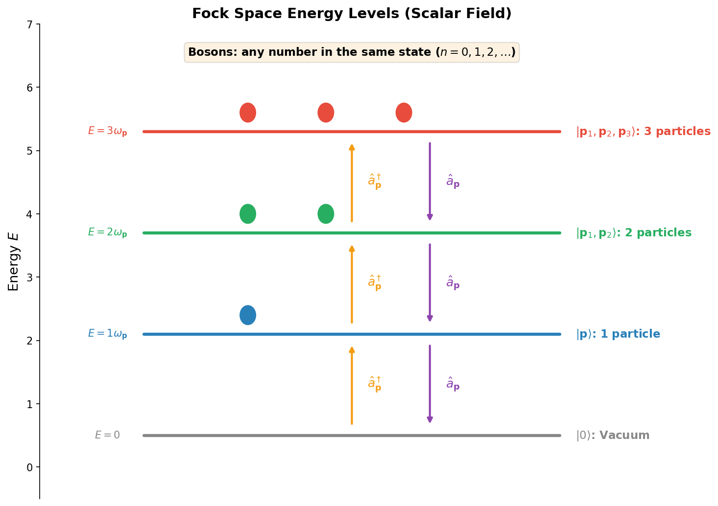
Fig. 4.3: Energy levels in Fock space. Particles are added by the creation operator \(\hat{a}^\dagger\) and removed by the annihilation operator \(\hat{a}\). Bosons can occupy the same state in any number.
✅ Comprehension Check: What fundamentally distinguishes Fock space from the Hilbert space of quantum mechanics?
Answer
The Hilbert space of quantum mechanics handles only states with a fixed particle number, but Fock space is constructed as the direct sum of all particle number sectors — particle number 0 (vacuum), 1, 2, and so on. This allows processes where particle number changes (creation and annihilation) to be described within a single unified framework.
✅ Comprehension Check: What does the state \(\hat{a}_{\mathbf{p}}^\dagger \hat{a}_{\mathbf{p}}^\dagger |0\rangle\) represent?
Answer
A state with two identical particles having momentum \(\mathbf{p}\). Since they are bosons, multiple particles are allowed in the same momentum state. (The precise normalization is \(\frac{1}{\sqrt{2}}(\hat{a}_{\mathbf{p}}^\dagger)^2 |0\rangle\), but care is needed with normalization conventions for continuous momentum labels.)
4.7 Number Operator and Hamiltonian
Number Operator
🟡 Lina: Remember how in the quantum mechanical harmonic oscillator, the number operator \(\hat{n} = a^\dagger a\) counted the quantum number of energy levels? In quantum field theory, we can also define a number operator.
This is an operator that counts "the number of particles with momentum \(\mathbf{p}\)." The total particle number is:
🔵 Kai: Let me verify. Acting \(\hat{N}_{\mathbf{p}}\) on the one-particle state \(|\mathbf{q}\rangle = \hat{a}_{\mathbf{q}}^\dagger |0\rangle\):
Using the commutation relation \(\hat{a}_{\mathbf{p}} \hat{a}_{\mathbf{q}}^\dagger = \hat{a}_{\mathbf{q}}^\dagger \hat{a}_{\mathbf{p}} + \delta^{(3)}(\mathbf{p} - \mathbf{q})\):
When \(\mathbf{p} = \mathbf{q}\), it returns "1 particle"; when \(\mathbf{p} \neq \mathbf{q}\), it returns "0 particles." It's properly counting particles!
Mode Expansion of the Hamiltonian
🟡 Lina: Now let's rewrite the Hamiltonian in terms of creation and annihilation operators. The Hamiltonian is:
Substituting equations (4.11a) and (4.12) and performing the spatial integration — the calculation is somewhat long, but let me explain the skeleton. For example, looking at the \(\hat{\pi}^2\) term: since \(\hat{\pi}\) contains both \(\hat{a}_{\mathbf{p}}\) and \(\hat{a}_{\mathbf{p}}^\dagger\), squaring it produces 4 types of terms: \(\hat{a}\hat{a}\), \(\hat{a}^\dagger\hat{a}^\dagger\), \(\hat{a}^\dagger\hat{a}\), and \(\hat{a}\hat{a}^\dagger\). Using Fourier orthogonality (4.15) in the spatial integral, the \(\hat{a}_{\mathbf{p}}\hat{a}_{\mathbf{q}}\) type terms contain \(\delta^{(3)}(\mathbf{p} + \mathbf{q})\), and the \(\hat{a}^\dagger\hat{a}\) type terms contain \(\delta^{(3)}(\mathbf{p} - \mathbf{q})\).
🔵 Kai: So two types appear: \(\delta^{(3)}(\mathbf{p} + \mathbf{q})\) and \(\delta^{(3)}(\mathbf{p} - \mathbf{q})\).
🟡 Lina: Right. Processing the \(\hat{\phi}^2\) and \((\nabla\hat{\phi})^2\) terms similarly, the \(\hat{a}\hat{a}\) type and \(\hat{a}^\dagger\hat{a}^\dagger\) type terms cancel between the three Hamiltonian terms — \(\frac{1}{2}\hat{\pi}^2\), \(\frac{1}{2}(\nabla\hat{\phi})^2\), \(\frac{1}{2}m^2\hat{\phi}^2\) — because the signs alternate (from \(\hat{\pi}^2\) comes a coefficient of \(-\omega_{\mathbf{p}}^2\), from \((\nabla\hat{\phi})^2\) comes \(+|\mathbf{p}|^2\), and from \(m^2\hat{\phi}^2\) comes \(+m^2\), but since \(\omega_{\mathbf{p}}^2 = |\mathbf{p}|^2 + m^2\) the total is zero). Ultimately only the \(\hat{a}^\dagger\hat{a}\) and \(\hat{a}\hat{a}^\dagger\) types survive.
⚪ Mei: The non-crossing terms exactly cancel — the relation \(\omega_{\mathbf{p}}^2 = |\mathbf{p}|^2 + m^2\) is doing the work.
🟡 Lina: Exactly. Since the free-field Lagrangian (4.1) doesn't explicitly depend on time \(t\), by Noether's theorem from Ch. 3, the energy (Hamiltonian) is a conserved quantity — meaning it's independent of time. So computing at \(t = 0\) gives the general result. The result is:
🔵 Kai: The first term is \(\omega_{\mathbf{p}} \hat{N}_{\mathbf{p}}\), so it's "particle number × energy for each mode" summed up. That makes sense. But what's the second term \(\frac{1}{2}\delta^{(3)}(\mathbf{0})\)? Isn't \(\delta^{(3)}(\mathbf{0})\) infinite?!
🟡 Lina: Good catch. This is the zero-point energy problem. We'll discuss it in detail in the next section.
✅ Comprehension Check: What do you get when you act the first term of the Hamiltonian (4.24), \(\int d^3p\, \omega_{\mathbf{p}}\, \hat{a}_{\mathbf{p}}^\dagger \hat{a}_{\mathbf{p}}\), on the one-particle state \(|\mathbf{q}\rangle\)?
Answer
\(\hat{H}|\mathbf{q}\rangle = \omega_{\mathbf{q}} |\mathbf{q}\rangle\) (ignoring the zero-point energy term). That is, the energy of a one-particle state with momentum \(\mathbf{q}\) is \(\omega_{\mathbf{q}} = \sqrt{|\mathbf{q}|^2 + m^2}\), satisfying the relativistic energy-momentum relation.
📝 Exercises:
- Calculation of the Hamiltonian mode expansion → Problem M-2. Expression of the Hamiltonian in Terms of Creation and Annihilation Operators
4.8 Zero-Point Energy and the Vacuum Problem
🟡 Lina: Let's look at equation (4.24) again.
Computing the energy of the vacuum state \(|0\rangle\):
🔵 Kai: This is doubly infinite, right? \(\delta^{(3)}(\mathbf{0})\) is infinite, and integrating \(\omega_{\mathbf{p}}\) over all momenta is also infinite.
🟡 Lina: That's right. There are two types of infinity:
-
Divergence of \(\delta^{(3)}(\mathbf{0})\): This originates from the infinite volume. Putting the system in a finite box \(V\) gives \(\delta^{(3)}(\mathbf{0}) \to V/(2\pi)^3\), so the energy density is finite. It's just that the total energy is infinite because space is infinitely large.
-
Divergence of \(\int d^3p\, \omega_{\mathbf{p}}\): This one is more serious. For \(|\mathbf{p}| \to \infty\), \(\omega_{\mathbf{p}} \to |\mathbf{p}|\), so high-momentum modes contribute infinitely. This is called the ultraviolet divergence.
🔵 Kai: The vacuum having infinite energy... isn't that physically problematic?
🟡 Lina: Good question. There are two ways of thinking about this.
Normal Ordering — A Practical Prescription
🟡 Lina: The first approach is: "In typical experiments, only energy differences are measurable, so let's redefine the vacuum energy to be zero." The mathematical operation that realizes this is normal ordering. It's denoted by \(:\!A\!:\).
Normal ordering means always placing creation operators \(\hat{a}^\dagger\) to the left of annihilation operators \(\hat{a}\). The constant terms that arise from commutation relations during the rearrangement are discarded. Here "constant terms" means purely numerical values containing no operators, which in quantum field theory are called c-numbers. The "c" stands for classical, referring to ordinary numbers like \(1\) or \(\delta^{(3)}(\mathbf{p}-\mathbf{q})\) that are not operators. In contrast, operators are sometimes called q-numbers (q for quantum). Why can we discard them? As I just said, typical experiments only measure energy differences, so adding or subtracting a constant from everything doesn't change physical predictions. Normal ordering corresponds to "setting the energy baseline to the vacuum."
🔵 Kai: I see, so it's an operation that aligns the "origin" of energy to the vacuum.
🟡 Lina: Right. Let's see this concretely. From commutation relation (4.13), \(\hat{a}_{\mathbf{p}} \hat{a}_{\mathbf{q}}^\dagger = \hat{a}_{\mathbf{q}}^\dagger \hat{a}_{\mathbf{p}} + \delta^{(3)}(\mathbf{p} - \mathbf{q})\). In normal ordering, we discard this \(\delta^{(3)}(\mathbf{p} - \mathbf{q})\) (c-number) and keep only the part with \(\hat{a}^\dagger\) moved to the left.
Applying this to the Hamiltonian:
The zero-point energy term has vanished!
⚪ Mei: So \(:\!\hat{H}\!:\, |0\rangle = 0\), meaning we've defined the vacuum energy to be zero.
🔵 Kai: But is it really okay to just "discard" the zero-point energy? Is it truly physically meaningless?
Is Zero-Point Energy Really Meaningless?
🟡 Lina: Actually, it's not entirely dismissible. The difference in zero-point energy is physically observable. The most famous example is the Casimir effect, which we'll calculate concretely at the end of this chapter.
Also, there's another serious issue. In general relativity, the absolute value of energy generates a gravitational field. So vacuum energy affects the expansion of the universe. The naively calculated vacuum energy density differs from the value inferred from cosmological observations by a factor of \(10^{120}\). This is called the cosmological constant problem and is one of the greatest unsolved problems in modern physics.
🔵 Kai: \(10^{120}\)?! That's beyond any reasonable discrepancy...
🟡 Lina: So normal ordering is a "practical prescription for carrying on with calculations," and the zero-point energy problem has not been completely solved. We'll touch on this again in Ch. 24 as one of the limitations of quantum field theory. I've summarized the normal ordering operation in Fig. 4.4 "Zero-point energy and normal ordering", so check it out.
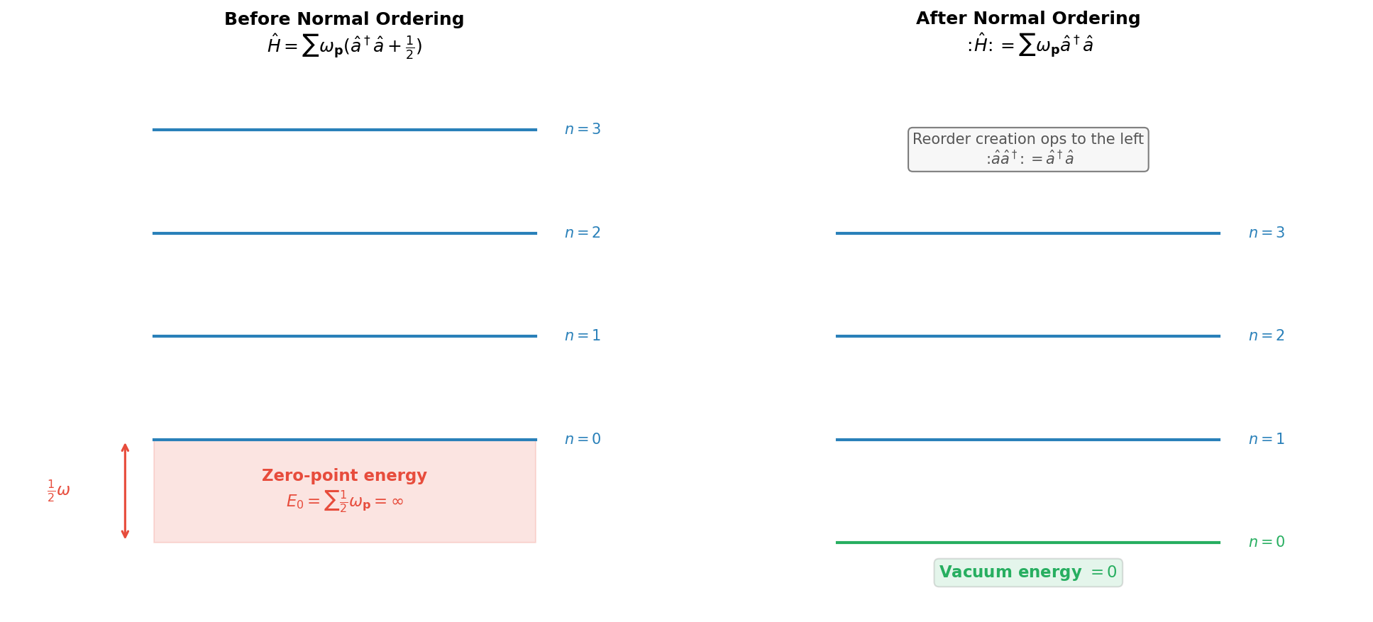
Fig. 4.4: Zero-point energy and normal ordering. Before normal ordering, an infinite zero-point energy exists, but normal ordering (rearranging creation operators to the left) allows redefining the vacuum energy to zero.
✅ Comprehension Check: What does the vacuum energy become when we take normal ordering \(:\!\hat{H}\!:\)? Why is that?
Answer
\(\langle 0|:\!\hat{H}\!:|0\rangle = 0\). In normal ordering, annihilation operators come to the right, so when acting on the vacuum, \(\hat{a}_{\mathbf{p}}|0\rangle = 0\) makes everything zero. This amounts to redefining the vacuum energy as zero.
4.9 Momentum Operator
🟡 Lina: Not only energy but also momentum can be expressed in terms of creation and annihilation operators. In Ch. 3, we derived momentum as the conserved quantity corresponding to spatial translation symmetry via Noether's theorem. The \(T^{0i}\) components of the canonical energy-momentum tensor \(T^{\mu\nu}\) give the momentum density. Specifically, \(T^{0i} = \frac{\partial\mathcal{L}}{\partial(\partial_0\phi)}\partial^i\phi = \pi\,\partial^i\phi\). A note of caution is needed here: in the QFT sign convention (\(\eta_{\mu\nu} = \mathrm{diag}(+1,-1,-1,-1)\)), raising a spatial index flips the sign. That is, \(\partial^i = \eta^{i\nu}\partial_\nu = \eta^{ii}\partial_i = (-1)\partial_i = -\partial_i\) (the diagonal metric means only the \(\nu = i\) term survives). Since \(\partial_i = \frac{\partial}{\partial x^i}\) is the ordinary spatial derivative (\(i\)-th component of \(\nabla\)), \(\partial^i\phi = -(\nabla\phi)_i\). Therefore \(T^{0i} = -\pi\,(\nabla\phi)_i\) and:
The negative sign comes from "raising a spatial index in the QFT metric gives a minus sign."
🔵 Kai: The negative sign comes from the sign convention. Can we intuitively check that this gives the correct momentum?
🟡 Lina: Good question. Let's intuitively verify the sign is correct. Consider a wave moving to the right in 1D, \(\phi \propto e^{-i(\omega t - px)} = e^{i(px - \omega t)}\) (\(p > 0\)). Then \(\nabla\phi = ip\,\phi\), \(\hat{\pi} = \dot{\phi} = -i\omega\,\phi\), so \(-\hat{\pi}\,\nabla\hat{\phi} = -(-i\omega)(ip)\,|\phi|^2 = \omega p\,|\phi|^2 > 0\), correctly returning positive momentum. Intuitively, \(\nabla\hat{\phi}\) represents "how much the field varies spatially," and \(\hat{\pi}\) represents "the vigor of the field's time variation," so their product gives "in which direction and with how much vigor the field wave is propagating" — that is, the momentum density. Substituting the mode expansions (4.11a), (4.12) and taking normal ordering — using Fourier orthogonality just as in the Hamiltonian calculation —
⚪ Mei: Comparing with the Hamiltonian (4.27), the structure is almost identical. Just \(\omega_{\mathbf{p}}\) replaced by \(\mathbf{p}\).
🔵 Kai: So it seems like we could combine energy and momentum into a "4-momentum" form.
🟡 Lina: Exactly. Combining them as a 4-momentum operator:
Acting on the one-particle state \(|\mathbf{q}\rangle\):
🔵 Kai: The one-particle state has energy \(\omega_{\mathbf{q}}\) and momentum \(\mathbf{q}\). It's exactly a relativistic particle of mass \(m\)! But if we act on the two-particle state \(|\mathbf{p}_1, \mathbf{p}_2\rangle\), does the energy become \(\omega_{\mathbf{p}_1} + \omega_{\mathbf{p}_2}\)?
🟡 Lina: That's right. In terms of the full 4-momentum: \(:\!\hat{P}^\mu\!: |\mathbf{p}_1, \mathbf{p}_2\rangle = (\omega_{\mathbf{p}_1} + \omega_{\mathbf{p}_2},\, \mathbf{p}_1 + \mathbf{p}_2)\,|\mathbf{p}_1, \mathbf{p}_2\rangle\). Both energy and momentum simply add up — this reflects the fact that for a free field there are no interactions, and particles behave independently. In quantum field theory, particles are not "things added to the field afterwards" but things that automatically appear as quantum excitations of the field. This is the realization of the worldview previewed in Quantum Mechanics Ch. 27 that "vibrational modes of the field are particles."
✅ Comprehension Check: What do you get when you act the 4-momentum operator \(:\!\hat{P}^\mu\!:\) on the one-particle state \(|\mathbf{q}\rangle\)? What does this mean?
Answer
\(:\!\hat{P}^\mu\!: |\mathbf{q}\rangle = (\omega_{\mathbf{q}}, \mathbf{q}) |\mathbf{q}\rangle\) is obtained. This means the one-particle state has energy \(\omega_{\mathbf{q}} = \sqrt{|\mathbf{q}|^2 + m^2}\) and momentum \(\mathbf{q}\), behaving as a particle of mass \(m\) satisfying the relativistic energy-momentum relation. The particle appeared automatically from field quantization and was not assumed by hand.
4.10 Complex Scalar Field and the Emergence of Antiparticles
🟡 Lina: So far we've been quantizing the real scalar field, but with a real scalar field only one type of "particle" appears. Yet in nature, every particle has an antiparticle. Where do antiparticles come from?
🔵 Kai: In Quantum Mechanics Ch. 27, there was a story about antiparticles being predicted from the Dirac equation.
🟡 Lina: Yes. But actually, antiparticles naturally emerge just by quantizing a simpler field — the complex scalar field.
Lagrangian of the Complex Scalar Field
🟡 Lina: The Lagrangian density for a complex scalar field \(\psi(x)\) can be written as:
🔵 Kai: It looks similar to the real scalar field Lagrangian (4.1), but \(\phi^2\) is replaced by \(\psi^\dagger \psi\). Why \(\psi^\dagger \psi\) instead of \(\psi^2\)?
🟡 Lina: Good question. Since \(\psi\) is complex, \(\psi^2\) would generally be complex. But the Lagrangian must be real (if the action \(S = \int d^4x\, \mathcal{L}\) isn't real, probability conservation breaks down). Since \(\psi^\dagger \psi = |\psi|^2\) is always real and non-negative, it's appropriate as a mass term. The kinetic term \((\partial_\mu \psi^\dagger)(\partial^\mu \psi)\) is paired as \(\psi^\dagger\) and \(\psi\) for the same reason.
⚪ Mei: The reality of the Lagrangian demands the combination \(\psi^\dagger \psi\).
🟡 Lina: Now let's look at the structure of the complex field a bit more. The complex field \(\psi\) can be written using two real scalar fields \(\phi_1, \phi_2\):
That is, the complex field has two independent real degrees of freedom. While the real scalar field had 1 degree of freedom, the complex scalar field has 2. This "doubling of degrees of freedom" is the key to particles and antiparticles appearing.
Mode Expansion — Two Types of Operators
🟡 Lina: In the mode expansion (4.11) of the real scalar field, there was only one type of pair, \(\hat{a}\) and \(\hat{a}^\dagger\). But since the complex field is not Hermitian (\(\hat{\psi} \neq \hat{\psi}^\dagger\)), two types of independent operators are needed.
🟡 Lina: Here I'll write in the Heisenberg picture including time dependence. In equation (4.11a) the combination \(e^{-i\omega_{\mathbf{p}} t + i\mathbf{p}\cdot\mathbf{x}}\) already appeared, and since this form comes up frequently in quantum field theory, let me formally introduce the compact notation using the 4-vector inner product \(p \cdot x\). This is standard notation used throughout quantum field theory, not just for complex fields, and we'll keep using it in all subsequent chapters. The real scalar field equation (4.11a) can also be written compactly as \(e^{-ip\cdot x}\) and \(e^{ip\cdot x}\) using this notation.
🔵 Kai: The 4-vector inner product uses the metric \(\eta_{\mu\nu}\) from Ch. 2, right?
🟡 Lina: Yes. Recall \(\eta_{\mu\nu} = \mathrm{diag}(+1, -1, -1, -1)\). For the 4-momentum \(p^\mu = (\omega_{\mathbf{p}},\, \mathbf{p})\) and 4-position \(x^\mu = (t,\, \mathbf{x})\), to compute the inner product we need to lower one index. Writing \(p_\mu = \eta_{\mu\nu} p^\nu\) (summing over \(\nu\)) in components: since the metric is diagonal, for \(\mu = 0\) we get \(p_0 = \eta_{00} p^0 = (+1) \times \omega_{\mathbf{p}} = \omega_{\mathbf{p}}\) so the time component is unchanged. For spatial components (\(\mu = 1, 2, 3\)), \(p_i = \eta_{i0}p^0 + \eta_{i1}p^1 + \eta_{i2}p^2 + \eta_{i3}p^3 = 0 + \cdots + (-1)p^i + \cdots = -p^i\) acquires a minus sign (the diagonal metric means all \(\mu \neq \nu\) terms are zero). So \(p_\mu = (\omega_{\mathbf{p}},\, -\mathbf{p})\).
🔵 Kai: Because the spatial components of the metric are \(-1\), lowering the index gives a minus on the spatial part.
🟡 Lina: Exactly. Therefore the 4-vector inner product — written here as \(p \cdot x\), which is shorthand for \(p_\mu x^\mu\) (summed by Einstein's convention) — is:
So \(e^{-ip\cdot x} = e^{-i\omega_{\mathbf{p}} t + i\mathbf{p}\cdot\mathbf{x}}\) corresponds to a positive frequency (positive energy) wave, and \(e^{ip\cdot x} = e^{i\omega_{\mathbf{p}} t - i\mathbf{p}\cdot\mathbf{x}}\) corresponds to a negative frequency wave.
⚪ Mei: Now the exponentials can be written neatly. So equation (4.11a) was just two terms with \(e^{-ip\cdot x}\) and \(e^{ip\cdot x}\).
🟡 Lina: Right. Now let me write the mode expansion of the complex field.
🔵 Kai: Two types, \(\hat{a}\) and \(\hat{b}\)! Why can't we just use \(\hat{a}\) alone? Also, why does \(\hat{b}^\dagger\) (a creation operator) pair with \(e^{ip\cdot x}\) (a negative frequency wave)?
🟡 Lina: Both are core questions. First question: for the real scalar field, Hermiticity \(\hat{\phi} = \hat{\phi}^\dagger\) meant the coefficient of \(e^{-ip\cdot x}\) (annihilation operator) and the coefficient of \(e^{ip\cdot x}\) (creation operator) were Hermitian conjugate pairs of the same operator. Here, "\(e^{-ip\cdot x}\) pairs with annihilation operator" and "\(e^{ip\cdot x}\) pairs with creation operator" is the convention we confirmed in equation (4.11a) for the real scalar field — \(e^{-ip\cdot x}\) is a positive-energy wave corresponding to "removing" a particle, while \(e^{ip\cdot x}\) corresponds to "adding" a particle. But the complex field \(\hat{\psi}\) is not Hermitian, so the coefficient of \(e^{-ip\cdot x}\) in \(\hat{\psi}\) (annihilation operator \(\hat{a}\)) and the coefficient of \(e^{ip\cdot x}\) (creation operator) must be a different type \(\hat{b}^\dagger\).
For the second question — why \(\hat{b}^\dagger\) pairs with \(e^{ip\cdot x}\): \(\hat{b}^\dagger\) is the operator that "creates" an antiparticle. Creating one antiparticle increases the system's energy by \(+\omega_{\mathbf{p}}\). Meanwhile, the time dependence of \(e^{ip\cdot x} = e^{i\omega_{\mathbf{p}} t - i\mathbf{p}\cdot\mathbf{x}}\) is \(e^{+i\omega t}\), and in the Heisenberg picture, "an operator that increases energy by \(\omega\)" acquires \(e^{+i\omega t}\) (same logic as \(\hat{a}^\dagger\) acquiring \(e^{+i\omega t}\) in the real scalar field). So it's natural for \(\hat{b}^\dagger\) to pair with \(e^{ip\cdot x}\).
⚪ Mei: So because the complex field isn't Hermitian, one type of operator pair isn't enough, and two independent types are needed.
🟡 Lina: Right. More specifically, recall from equation (4.32) that \(\psi\) is made from two real fields \(\phi_1\) and \(\phi_2\). Roughly speaking, "2 real degrees of freedom → 2 types of operators." However, strictly speaking \(\hat{a}\) and \(\hat{b}\) don't correspond simply to \(\phi_1\) and \(\phi_2\) but are in a mixed form. The commutation relations are:
All other commutators (\([\hat{a}, \hat{b}]\), \([\hat{a}, \hat{b}^\dagger]\), etc.) are zero. The \(\hat{a}\)-type and \(\hat{b}\)-type are completely independent.
Hamiltonian and Particles/Antiparticles
🟡 Lina: The normal-ordered Hamiltonian is:
🔵 Kai: Both \(\hat{a}\) particles and \(\hat{b}\) particles have energy \(\omega_{\mathbf{p}} = \sqrt{|\mathbf{p}|^2 + m^2}\), with the same mass \(m\)!
🟡 Lina: Yes. The particles created by \(\hat{a}_{\mathbf{p}}^\dagger\) are called "particles," and those created by \(\hat{b}_{\mathbf{p}}^\dagger\) are called "antiparticles." Particles and antiparticles have the same mass but opposite signs of conserved charge.
\(U(1)\) Symmetry and Conserved Charge
🟡 Lina: The complex scalar field Lagrangian (4.31) has a symmetry that the real scalar field doesn't. Under the phase transformation:
the Lagrangian is invariant. Since \(\alpha\) is a constant, it passes through derivatives, and \(e^{-i\alpha} \cdot e^{i\alpha} = 1\) leaves \(\psi^\dagger \psi\) invariant. This transformation of "multiplying by a constant phase \(e^{i\alpha}\)" is called a \(U(1)\) transformation. \(U(1)\) is the set of "all complex numbers with absolute value 1," which is exactly \(e^{i\alpha}\) (\(\alpha\) being any real number). The "\(U\)" stands for unitary, meaning "a transformation that preserves absolute value," and the "\(1\)" means "1-dimensional complex number."
⚪ Mei: This is a continuous symmetry. Since \(\alpha\) can be varied continuously.
🟡 Lina: Right. And having a continuous symmetry means we can use Noether's theorem from Ch. 3. Noether's theorem says a conserved quantity corresponds to each continuous symmetry. Computing the conserved charge corresponding to this \(U(1)\) symmetry (see exercise Problem M-4. Quantization of the Complex Scalar Field and Particles/Antiparticles for the explicit derivation):
🔵 Kai: The number of particles minus the number of antiparticles! So even if a particle and antiparticle annihilate each other, \(Q\) doesn't change — \(+1\) and \(-1\) cancel to net zero. But if only a single particle were created, \(Q\) would change, right? Is that not allowed?
🟡 Lina: Good question. Since \(Q\) is a conserved quantity, a particle cannot be created alone. Particles and antiparticles must always be created and annihilated in pairs. This is the physical meaning of "conserved charge." And since the real scalar field has \(\phi = \phi^\dagger\), there's no \(U(1)\) symmetry and no conserved charge is defined (or formally writing one gives zero). In other words, the real scalar field's particle "is its own antiparticle." The complex scalar field, on the other hand, has \(\psi \neq \psi^\dagger\), so \(U(1)\) symmetry emerges, and particles and antiparticles are distinguished by the sign of charge. Let me summarize the differences between real and complex scalar fields in a table.
Table 4.5: Comparison of real and complex scalar fields
| Real scalar field \(\phi\) | Complex scalar field \(\psi\) | |
|---|---|---|
| Hermiticity | \(\hat{\phi} = \hat{\phi}^\dagger\) | \(\hat{\psi} \neq \hat{\psi}^\dagger\) |
| Types of operators | \(\hat{a}\) only | \(\hat{a}\) and \(\hat{b}\) |
| Types of particles | 1 type (particle = antiparticle) | 2 types (particle and antiparticle) |
| \(U(1)\) symmetry | None | Present |
| Conserved charge | \(Q = 0\) | \(Q = N_a - N_b\) |
⚪ Mei: A beautiful contrast. Looking at the table, you can see the differences cascade from the presence or absence of Hermiticity.
Charge Conjugation
🟡 Lina: The operation that swaps particles and antiparticles is called charge conjugation. It's denoted by \(C\).
The Hamiltonian (4.36) is symmetric in \(\hat{a}\) and \(\hat{b}\), so it's invariant under \(C\). But the conserved charge (4.38):
flips sign.
🔵 Kai: Swapping particles and antiparticles only changes the sign of charge. Mass and energy remain the same.
🟡 Lina: I've summarized the overall structure in Fig. 4.5 "Complex scalar field and the emergence of antiparticles". This is one consequence of the CPT theorem — the theorem stating that performing all three operations of charge conjugation (C), spatial inversion (P), and time reversal (T) simultaneously always leaves physical laws invariant. From this theorem, it follows that particles and antiparticles must have the same mass. This has been confirmed experimentally to extremely high precision. We'll discuss the CPT theorem in detail in Ch. 10.
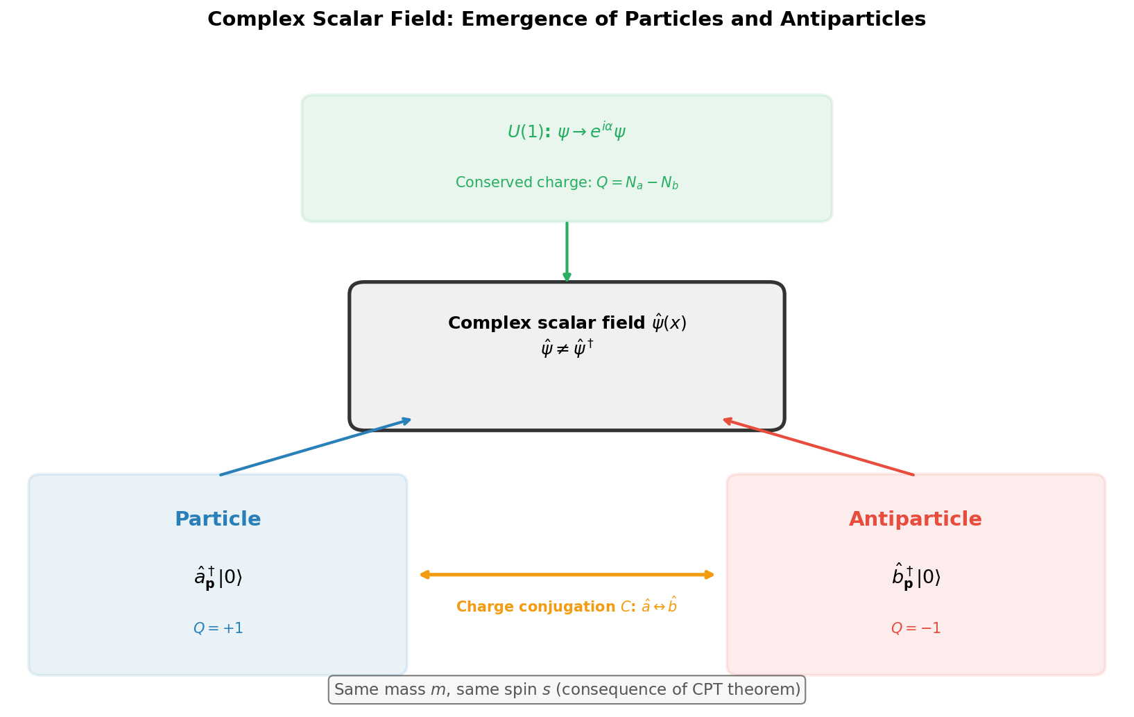
Fig. 4.5: Complex scalar field and the emergence of antiparticles. Quantization of the complex scalar field naturally produces particles (\(\hat{a}^\dagger\)) and antiparticles (\(\hat{b}^\dagger\)). \(U(1)\) symmetry generates a conserved charge, and charge conjugation \(C\) swaps particles and antiparticles.
✅ Comprehension Check: Under charge conjugation \(C\), how do the Hamiltonian (4.36) and the conserved charge \(\hat{Q}\) (4.38) transform?
Answer
The Hamiltonian is symmetric in \(\hat{a}\) and \(\hat{b}\), so it's invariant under \(C\). Meanwhile, the conserved charge flips sign: \(\hat{Q} \to -\hat{Q}\). This means swapping particles and antiparticles leaves mass and energy unchanged but reverses the sign of charge.
✅ Comprehension Check: In the quantization of the complex scalar field, why are two types of creation/annihilation operators (\(\hat{a}\), \(\hat{b}\)) needed? Explain in one sentence.
Answer
Since the complex field \(\hat{\psi}\) is not Hermitian (\(\hat{\psi} \neq \hat{\psi}^\dagger\)), independent operators must be assigned to the positive and negative frequency parts, each responsible for the creation and annihilation of particles and antiparticles respectively.
📝 Exercises:
- Derivation of the conserved charge for the complex scalar field → Problem M-4. Quantization of the Complex Scalar Field and Particles/Antiparticles
4.11 Casimir Effect — Zero-Point Energy Really Exists
🟡 Lina: Earlier I said we "discarded the zero-point energy with normal ordering," but the difference in zero-point energy is physically observable. The most direct evidence is the Casimir effect, predicted in 1948 by Hendrik Casimir and later confirmed experimentally.
🔵 Kai: Zero-point energy is observable? How?
Setup: Two Parallel Metal Plates
🟡 Lina: Take a look at the setup in Fig. 4.6 "Setup for the Casimir effect". Consider placing two perfectly conducting parallel metal plates separated by distance \(d\) in vacuum.
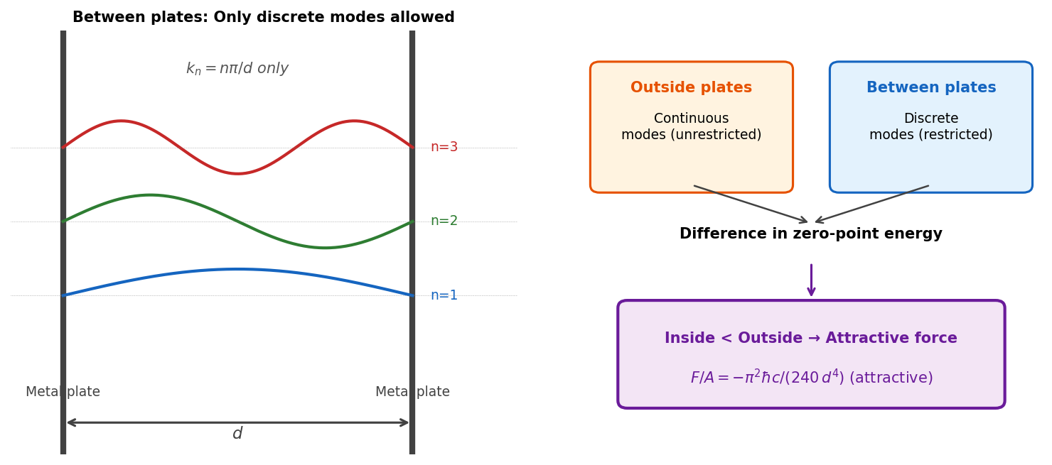
Fig. 4.6: Setup for the Casimir effect. Between the metal plates, boundary conditions allow only discrete modes (\(k_n = n\pi/d\)). Outside, continuous modes exist. The difference in zero-point energy density between inside and outside manifests as an attractive force (Casimir force) pulling the plates together.
Between the plates, the field's vibrational modes are subject to boundary conditions. Since the field must vanish at the conductor surfaces (be a "node" of the wave), only discrete wave numbers are allowed. It's exactly like the vibrations of a string fixed at both ends, where only wavelengths that are integer fractions of the string length are permitted.
Outside the metal plates, wave numbers are continuous.
⚪ Mei: Since the allowed modes are restricted between the plates, the zero-point energy density differs between inside and outside.
🟡 Lina: Exactly. The difference in zero-point energy exerts a force on the metal plates.
Calculation in 1D
🟡 Lina: To see the essence, let's first calculate for a massless scalar field in 1D. Casimir originally considered the electromagnetic field (photon field), but the essential physics lies in the difference of zero-point energy for a massless field, so we'll discuss a \(m = 0\) scalar field here (in 3D electromagnetism, the polarization degrees of freedom add a factor of 2, but the \(d\)-dependence is the same). Setting \(m = 0\) simplifies things to \(\omega_n = \sqrt{k_n^2 + m^2} = k_n = n\pi/d\). The zero-point energy between the plates is:
🔵 Kai: \(\sum_{n=1}^{\infty} n = 1 + 2 + 3 + \cdots\) diverges, right?
🟡 Lina: Yes. But here's where we make a physical argument. The calculation ahead is somewhat long, so let me state the goal first. When we subtract the zero-point energy without plates (continuous integral) from the zero-point energy with plates (discrete sum), the divergent parts cancel and only a finite value remains — finding that finite value is the purpose of this calculation.
Real metal plates become transparent to electromagnetic waves of very short wavelength (very high energy). So high-frequency modes aren't affected by the boundary conditions. To mathematically implement this, we use a technique called regularization.
Specifically, we insert an exponential damping factor \(e^{-\epsilon n}\) (\(\epsilon > 0\) is a small positive number):
🔵 Kai: Wait, why choose the form \(e^{-\epsilon n}\)? Would a different damping factor give the same result?
🟡 Lina: Good question. Actually, any function that suppresses large \(n\) gives the same finite physical part (the \(-1/12\) term). For example, \(e^{-\epsilon n^2}\) or cutting off at some value \(N\) would all give different forms for the divergent part, but the finite part remains unchanged. This is the core of regularization — physical results don't depend on the regularization method. In exercise Problem A-1. Quantitative Calculation of the 1-Dimensional Casimir Effect, you'll confirm that a different method (zeta function regularization) also gives the same \(-1/12\). We use \(e^{-\epsilon n}\) here because it allows easy calculation using the geometric series formula.
🔵 Kai: I see, we're choosing for computational convenience, and the physical answer doesn't depend on the method.
🟡 Lina: Exactly. This sum can be computed. Differentiating both sides of the geometric series \(\sum_{n=0}^{\infty} x^n = \frac{1}{1-x}\) (\(|x| < 1\)) with respect to \(x\) gives \(\sum_{n=1}^{\infty} n\, x^{n-1} = \frac{1}{(1-x)^2}\), and multiplying both sides by \(x\):
Since \(x = e^{-\epsilon} < 1\) for \(\epsilon > 0\), this formula applies. Let's expand with \(x = e^{-\epsilon}\).
⚪ Mei: A formula obtained by differentiating the geometric series.
🟡 Lina: Right. The goal is to separate "the part that diverges as \(\epsilon \to 0\)" from "the finite part independent of \(\epsilon\)." Let's proceed systematically with the Taylor expansion. Since \(e^{-\epsilon} \approx 1 - \epsilon + \frac{\epsilon^2}{2} - \frac{\epsilon^3}{6} + \cdots\), the denominator is:
Therefore:
🔵 Kai: Let me organize this. What we want to do is expand \(\sum n\,e^{-\epsilon n} = \frac{e^{-\epsilon}}{(1-e^{-\epsilon})^2}\) in powers of \(\epsilon\) to separate the divergent and finite parts, right?
🟡 Lina: Exactly. The goal is to "expand \(\frac{e^{-\epsilon}}{(1-e^{-\epsilon})^2}\) in powers of \(\epsilon\) and separate the \(\epsilon^{-2}\) (divergent term) from the \(\epsilon^0\) (finite term)." Using \((1-u)^{-2} \approx 1 + 2u + 3u^2 + \cdots\) (from the geometric series \(\frac{1}{1-u} = 1 + u + u^2 + \cdots\) (valid for \(|u| < 1\)), differentiating both sides with respect to \(u\) gives \(\frac{1}{(1-u)^2} = 1 + 2u + 3u^2 + \cdots\). Here \(u \approx \epsilon/2\) and \(\epsilon\) is small, so \(|u| < 1\) is satisfied) applied to \(u = \frac{\epsilon}{2} - \frac{\epsilon^2}{6} + \cdots\).
🔵 Kai: Since \(u\) is first order in \(\epsilon\), \(u^2\) only contributes at \(\epsilon^2\) and higher.
🟡 Lina: Exactly. In the expression above, \(1 - e^{-\epsilon} \approx \epsilon\left(1 - \frac{\epsilon}{2} + \frac{\epsilon^2}{6} - \cdots\right)\). Defining \(u \equiv \frac{\epsilon}{2} - \frac{\epsilon^2}{6} + \cdots\), we can write \(1 - e^{-\epsilon} = \epsilon(1 - u)\). Therefore \(\frac{1}{(1-e^{-\epsilon})^2} = \frac{1}{\epsilon^2} \cdot \frac{1}{(1 - u)^2}\). Substituting \(u = \frac{\epsilon}{2} - \frac{\epsilon^2}{6} + \cdots\) into \(\frac{1}{(1-u)^2} = 1 + 2u + 3u^2 + \cdots\): the \(\epsilon^0\) term is \(1\), the \(\epsilon^1\) term is \(2 \times \frac{1}{2} = 1\), the \(\epsilon^2\) term is \(2 \times (-\frac{1}{6}) + 3 \times (\frac{1}{2})^2 = -\frac{1}{3} + \frac{3}{4} = \frac{5}{12}\). So \(\frac{1}{(1-u)^2} \approx 1 + \epsilon + \frac{5}{12}\epsilon^2 + \cdots\), giving:
Next multiply by the numerator \(e^{-\epsilon} \approx 1 - \epsilon + \frac{\epsilon^2}{2} - \cdots\). That is, expand \(\frac{e^{-\epsilon}}{(1-e^{-\epsilon})^2} \approx \frac{1}{\epsilon^2} \times (1 - \epsilon + \frac{\epsilon^2}{2} - \cdots)(1 + \epsilon + \frac{5\epsilon^2}{12} + \cdots)\). Since the overall factor is \(\frac{1}{\epsilon^2}\), we just need to organize the product of the two brackets by powers of \(\epsilon\) — same idea as "expanding polynomials" from high school math.
\(\epsilon^0\) term (= overall \(\epsilon^{-2}\)): \(1 \times 1 = 1\) → overall \(\frac{1}{\epsilon^2}\)
\(\epsilon^1\) term (= overall \(\epsilon^{-1}\)): \(1 \times \epsilon + (-\epsilon) \times 1 = \epsilon - \epsilon = 0\) → vanishes
🔵 Kai: Oh, the \(\epsilon^{-1}\) term exactly cancels!
🟡 Lina: Yes, this isn't coincidental but derives from symmetry properties of this function. For the \(\epsilon^2\) term (= overall \(\epsilon^0\)): collecting three combinations.
- \(1 \times \frac{5\epsilon^2}{12} = \frac{5\epsilon^2}{12}\)
- \((-\epsilon) \times \epsilon = -\epsilon^2\)
- \(\frac{\epsilon^2}{2} \times 1 = \frac{\epsilon^2}{2}\)
Adding: \(\left(\frac{5}{12} - 1 + \frac{1}{2}\right)\epsilon^2 = \left(\frac{5}{12} - \frac{12}{12} + \frac{6}{12}\right)\epsilon^2 = -\frac{1}{12}\epsilon^2\). Multiplying by the overall \(\frac{1}{\epsilon^2}\) gives \(-\frac{1}{12}\). Summarizing:
The expansion thus far has given us equation (4.43). The important point is that the divergent \(1/\epsilon^2\) and finite \(-1/12\) are cleanly separated. (In exercise Problem A-1. Quantitative Calculation of the 1-Dimensional Casimir Effect, you'll confirm the same calculation with a different regularization method (zeta function regularization) and extend to 3D.)
⚪ Mei: The divergent and finite parts are completely separated by powers of \(\epsilon\).
🟡 Lina: But this divergent term corresponds to "free-space zero-point energy" that exists even without the metal plates. Think about it — even in infinite space without plates, each mode has zero-point energy \(\frac{1}{2}\omega\), and summing over all modes gives the same kind of divergence. Introducing metal plates only changes which modes are allowed through discretization, causing some modes to "drop out." So taking the difference between the zero-point energy with and without plates, the \(1/\epsilon^2\) divergence common to both cancels, and only the finite \(-1/12\) part remains — this is the effect of the boundary conditions.
🔵 Kai: More concretely, the zero-point energy without plates also contains a \(1/\epsilon^2\) term when computed with the same regularization, but doesn't contain the \(-1/12\) part — so subtracting gives only \(-1/12\)?
🟡 Lina: That understanding is correct. More precisely, without plates the modes are continuous, so the zero-point energy is an integral \(\int dk\, \frac{1}{2}\omega_k\) rather than a sum. Computing this integral with the same regularization produces a \(d\)-independent divergence (corresponding to \(1/\epsilon^2\)) but no finite correction like \(-1/12\). The reason is that \(-1/12\) arises from "the error when approximating the discrete sum \(\sum_{n=1}^\infty n\) by the corresponding continuous integral \(\int_0^\infty n\,dn\)." The integral \(\int_0^\infty n\,dn\) itself diverges, but the difference between sum and integral \(\sum n - \int n\,dn\) is finite, and its value is exactly \(-1/12\) (this is a mathematical result known as the Euler-Maclaurin formula). Without plates, it's an integral from the start, so this "difference between sum and integral" doesn't exist. In other words, the Casimir energy is defined as the difference between "the zero-point energy with plates (discrete sum)" minus "the zero-point energy without plates (continuous integral)," and that difference corresponds to \(-1/12\). Multiplying by the prefactor \(\frac{\pi}{2d}\) from equation (4.42):
🔵 Kai: Negative! Making \(d\) smaller lowers the energy (makes it more negative), so there's a force pushing the plates closer together?
🟡 Lina: Exactly. In high school physics you learned "conservative force is minus the position derivative of potential energy." By the same logic, the force from changing the plate separation is \(F = -\frac{\partial E_{\text{Casimir}}}{\partial d}\). Taking the direction of increasing \(d\) as positive, \(F < 0\) means toward closer plates — an attractive force.
⚪ Mei: The divergence cancelled, leaving only a finite force depending on \(d\) — this is the true nature of the Casimir force.
Result in 3D
🟡 Lina: In real 3-dimensional space, the momentum parallel to the plates \(\mathbf{p}_\parallel = (p_y, p_z)\) is continuous, and only the wave number perpendicular to the plates is discretized to \(k_n = n\pi/d\). That is, for each discrete mode \(n\), waves of all momenta can propagate parallel to the plates. The total zero-point energy involves both an integral over \(\mathbf{p}_\parallel\) and a sum over \(n\), making the calculation more complex than the 1D case. Since each mode's energy is \(\omega = \sqrt{k_n^2 + |\mathbf{p}_\parallel|^2}\), the \(\mathbf{p}_\parallel\) integral introduces additional dimension-dependence.
🔵 Kai: Only the direction perpendicular to the plates gets discretized, while waves can propagate freely in the parallel directions.
🟡 Lina: Right. Roughly speaking, in 1D there was only a discrete mode sum, but in 3D for each discrete mode \(n\) we must integrate over all parallel momenta \(\mathbf{p}_\parallel\). This additional 2D integral changes the power of \(d\) — by dimensional analysis, in 1D the energy goes as \(\propto 1/d\) so the force is \(\propto 1/d^2\), but in 3D the integration over parallel directions produces an extra \(1/d^2\), making the force per unit area \(\propto 1/d^4\). The numerical factor also changes from \(-1/12\) to \(\pi^2/720\). I'll leave the detailed derivation to the exercise (advanced part of Problem A-1. Quantitative Calculation of the 1-Dimensional Casimir Effect), but the result is:
This is in natural units (\(\hbar = c = 1\)). To compare with experiment, we restore \(\hbar\) and \(c\) (in natural units \([F/A] = [\text{length}]^{-4}\), while in SI units \([F/A] = [\text{energy}] \cdot [\text{length}]^{-4}\), so multiplying by one factor of \(\hbar c\) (with dimensions \([\text{energy}] \cdot [\text{length}]\)) makes the dimensions match):
🔵 Kai: It's inversely proportional to \(d^4\), so the closer the plates, the stronger the force. How large is it specifically?
🟡 Lina: For \(d = 1\,\mu\mathrm{m}\), \(F/A \approx 1.3 \times 10^{-3}\,\mathrm{N/m^2}\). Very small, but measurable.
🟡 Lina: Let me summarize the 1D and 3D results in a table.
Table 4.6: Summary of the Casimir effect
| 1D (\(\hbar = c = 1\)) | 3D (realistic) | |
|---|---|---|
| Casimir force | \(F = -\dfrac{\pi}{24d^2}\) | \(F/A = -\dfrac{\pi^2\hbar c}{240\,d^4}\) |
| Distance dependence | \(\propto d^{-2}\) | \(\propto d^{-4}\) |
| Direction of force | Attractive (pulls plates together) | Attractive (pulls plates together) |
⚪ Mei: In 1D it's \(d^{-2}\), in 3D it's \(d^{-4}\) — the distance dependence steepens with increasing dimension.
Experimental Verification
🟡 Lina: The Casimir effect was first precisely measured in 1997 by Steve Lamoreaux. He measured the force between a metal plate and a metal sphere, confirming agreement with the theoretical prediction to within 5%. Subsequent experiments have confirmed agreement to better than 1% precision.
🔵 Kai: Zero-point energy really exists and produces a physical force. Amazing...
⚪ Mei: So discarding the zero-point energy with normal ordering was purely a computational convenience, and the difference in zero-point energy is a real physical quantity.
🟡 Lina: Exactly. The Casimir effect is one of the beautiful examples where quantum field theory predictions agree with experiment. And at the same time, it demonstrates that the concept of vacuum energy is not merely a mathematical artifact but has physical reality.
✅ Comprehension Check: In the 3D Casimir force formula \(F/A = -\pi^2 \hbar c / (240\, d^4)\), how does the force change if the plate separation \(d\) is halved?
Answer
Since the force is inversely proportional to \(d^4\), halving \(d\) increases the force by \(2^4 = 16\) times. The Casimir force grows extremely rapidly at short distances, becoming measurable at sub-micrometer scales.
✅ Comprehension Check: Explain the physical reason why the Casimir effect is "attractive" from the perspective of zero-point energy.
Answer
Between the metal plates, boundary conditions restrict the allowed vibrational modes (long-wavelength modes cannot fit). Therefore, the zero-point energy density between the plates is smaller than outside. This energy difference between inside and outside manifests as a force in the direction of bringing the plates closer (attractive). Narrowing the plate separation further restricts modes and lowers the energy, so the system tends toward lower energy — that is, the direction where plates approach each other.
📝 Exercises:
- Regularization calculation of 1D Casimir energy → Problem A-1. Quantitative Calculation of the 1-Dimensional Casimir Effect
4.12 Summary of This Chapter
🟡 Lina: Let's review today's content.
⚪ Mei: Let me organize.
-
Canonical quantization: We promoted the classical field \(\phi\) and conjugate momentum \(\pi\) to operators and imposed the equal-time commutation relation \([\hat{\phi}(\mathbf{x}), \hat{\pi}(\mathbf{y})] = i\,\delta^{(3)}(\mathbf{x} - \mathbf{y})\).
-
Fourier expansion and harmonic oscillators: Fourier transforming the Klein-Gordon field makes each momentum mode an independent harmonic oscillator. We introduced creation and annihilation operators \(\hat{a}_{\mathbf{p}}^\dagger\), \(\hat{a}_{\mathbf{p}}\) for each mode.
-
Fock space and particle picture: Particle states are constructed by applying creation operators to the vacuum \(|0\rangle\). Bose-Einstein statistics is automatically derived from the commutation relations.
🔵 Kai: And the key points of the second half were —
- Zero-point energy: The Hamiltonian contains an infinite zero-point energy. It's practically handled by normal ordering, but the difference in zero-point energy is physically observable as the Casimir effect. It was striking that something we "discarded" can be measured as a force. But conversely, what can be discarded is only "the part that doesn't affect differences," not just anything, right?
🟡 Lina: Exactly right, sharp observation. Normal ordering is an operation that "sets the baseline to zero," but differences from the baseline are physically meaningful. The Casimir effect is precisely an example where that difference manifests as a force. And as the cosmological constant problem shows, when considering gravity the baseline itself becomes meaningful — that's a deep unsolved problem.
⚪ Mei: And the fifth point was —
-
Complex scalar field and antiparticles: In the quantization of a complex field, two types of operators \(\hat{a}\), \(\hat{b}\) appear, and particles and antiparticles naturally emerge. \(U(1)\) symmetry generates a conserved charge, and charge conjugation swaps particles and antiparticles.
-
Casimir effect: Differences in zero-point energy are physically observable. The restriction of allowed modes between metal plates produces a force pulling the plates together. This is direct evidence that zero-point energy is not merely a mathematical artifact but has physical reality.
⚪ Mei: Summarizing everything in one phrase: the heart of quantum field theory is "field excitations are particles." Without putting particles in by hand, just quantizing a field produces particles. And making the field complex produces antiparticles too. Furthermore, zero-point energy — a byproduct of quantization — is also observable as the Casimir effect, just as Lina showed us.
🟡 Lina: In the next chapter, we'll apply the same canonical quantization procedure to the Dirac field — the field of spin-1/2 fermions. There, instead of commutation relations, anti-commutation relations appear, and Fermi-Dirac statistics is automatically derived. The contrast with the scalar field will be very striking.
Preview of Next Chapter
Ch. 5 Quantization of the Dirac Field — Anti-commutation Relations for Fermions
When quantizing a spin-1/2 field, we must impose anti-commutation relations \(\{\hat{\psi}, \hat{\psi}^\dagger\} = \delta^{(3)}\) instead of commutation relations. Why? And how does Pauli's exclusion principle follow from this? Through a vivid contrast with the scalar field, we reveal the deep connection between spin and statistics.
References
- Quantum Field Theory for the Gifted Amateur (Lancaster & Blundell) Chapter 12: "The canonical quantization of fields"
- Quantum Field Theory for the Gifted Amateur (Lancaster & Blundell) Chapter 13: "Fields with more than one component"
- Quantum Field Theory (David Tong, Cambridge lecture notes) Chapter 2: "Classical Field Theory" & Chapter 3: "Canonical Quantization"
- 場の量子論——不変性と自由場を中心にして(場 上) Chapter 10: "正準量子化の方法" & Chapter 11: "スカラー場の量子化"
- Quantum Field Theory and the Standard Model (Schwartz) Chapter 2: "Lorentz invariance and second quantization"
Exercises
📝 Exercises:
- Derivation of equal-time commutation relations → Problem M-1. Derivation of Creation and Annihilation Operator Commutation Relations from Equal-Time Commutation Relations
- Calculation of the Hamiltonian mode expansion → Problem M-2. Expression of the Hamiltonian in Terms of Creation and Annihilation Operators
- Derivation of the conserved charge for the complex scalar field → Problem M-4. Quantization of the Complex Scalar Field and Particles/Antiparticles
- Regularization calculation of 1D Casimir energy → Problem A-1. Quantitative Calculation of the 1-Dimensional Casimir Effect
Feedback on this page
Let us know if something was unclear, incorrect, or could be improved.