Chapter 7: Why Are Atoms Stable? — The Birth of Quantum Mechanics¶
Story so far: In Chapters 5–6, we traced the trunk of relativity. Special relativity rewrote time and space, and general relativity described gravity as the curvature of spacetime. From here, we return to the other crisis left open in Ch. 4—the atomic stability problem—and retrace the trunk of quantum theory.
Goals of This Chapter
- Quantum mechanics is treated systematically in Quantum Mechanics Ch. 1
- In this chapter, we receive those results in compressed form while taking particular care to establish the structure that directly connects to string theory—quantization via the ladder operators of the harmonic oscillator—and identify the confluence point with the relativity trunk
How to Read This Chapter
This chapter is written assuming you have read Quantum Mechanics Prologue. The crisis of classical physics, the Bohr model, the Schrödinger equation, commutation relations and the uncertainty principle, the algebraic solution of the harmonic oscillator, and spin are all derived in Quantum Mechanics, so here we summarize results only. In their place, we emphasize the structures that reappear in string theory—"ladder operators and the energy level ladder" and "zero-point energy as the sum of minimum energies"—and organize the "incompatibility of the Schrödinger equation with special relativity" treated in Quantum Mechanics Ch. 27 so as to connect it to the flow of Part III of this book.
%%{init: {"theme": "default", "themeCSS": ".edgePath .path, .flowchart-link { stroke-width: 2px !important; }"}}%%
flowchart LR
    subgraph A["Developed in Quantum Mechanics"]
        A1["Crisis of classical physics<br/>Planck / Bohr"]
        A2["Wave function and<br/>Schrödinger equation"]
        A3["Commutation relations and<br/>uncertainty principle"]
        A4["Harmonic oscillator<br/>(algebraic solution)"]
        A5["Spin<br/>(Pauli matrices)"]
    end

    subgraph B["Original content emphasized in this chapter"]
        B1["Ladder operators<br/>a, a†"]
        B2["Zero-point energy<br/>ℏω/2"]
        B3["Infinitely many harmonic oscillators<br/>= quantization of the string"]
    end

    subgraph C["Bridge to the next chapter"]
        C1["Collision with relativity<br/>→ Quantum field theory (Chapter 8)"]
    end

    A4 --> B1
    B1 --> B2
    B2 --> B3
    A2 --> C1
    A3 --> C1
Fig. 7.1: Positioning of this chapter and its relationship to preceding and following chapters
7.1 Summary of Key Points: The Crisis of Classical Physics and the Bohr Model¶
🟡 Lina: Now that we've traced the trunk of relativity, let's return to the trunk of quantum theory. The starting point is the "breakdown of classical physics" we touched on in Ch. 4. At the end of the 19th century, phenomena appeared one after another that couldn't be explained within the framework of Newtonian mechanics and Maxwell's electromagnetism. I'll leave the details to Quantum Mechanics Ch. 1 and summarize in Table 7.1 "The crises of classical physics and their resolutions" only the conclusions needed for Part III.
Table 7.1: The crises of classical physics and their resolutions
| Crisis | Core contradiction | Resolver | Key equation |
|---|---|---|---|
| Ultraviolet catastrophe of blackbody radiation | Classical prediction diverges at high frequencies | Planck (1900) | \(E = nh\nu\) |
| Photoelectric effect | Frequency, not intensity, is decisive | Einstein (1905) | \(K = h\nu - W\) |
| Atomic stability | Electron spirals in within \(10^{-11}\) seconds | Bohr (1913) | \(E_n = -13.6\,\mathrm{eV}/n^2\) |
🔵 Kai: All three involve Planck's constant \(h\), right? But Bohr's assumptions—"no radiation in stationary states" and "angular momentum is an integer multiple of \(\hbar\)"—aren't they just postulated without any explanation of why?
🟡 Lina: Yes. The constant running through all of them is \(h \approx 6.626\times 10^{-34}\,\mathrm{J\cdot s}\) and \(\hbar = h/(2\pi)\). Nature behaves not continuously but discretely (in jumps)—this is the starting point of everything. In Bohr's hydrogen atom model, the allowed orbital radii of the electron are
—only discrete values are permitted. \(a_0\) is called the Bohr radius and corresponds to the radius of the innermost orbit (\(n = 1\)). The corresponding energy levels are \(E_n = -13.6\,\mathrm{eV}/n^2\) from the table, where \(n = 1\) is the lowest energy (ground state)—explaining that the atom cannot fall below this.
✅ Comprehension Check: What physical constant appears in common across the three crises of classical physics (blackbody radiation, photoelectric effect, atomic stability)? What fundamental property of nature does it signify?
Answer
The constant appearing in common is Planck's constant \(h\) (or \(\hbar = h/(2\pi)\)). This indicates that nature behaves not continuously but discretely (in jumps). Energy and angular momentum cannot take arbitrary values—only discrete values in units of \(h\) are permitted.
⚪ Mei: So Bohr's hypothesis was confirmed to "agree with experiment," but "why that condition holds" was imported from outside the model—meaning the theory was incomplete.
🟡 Lina: Exactly. The answer to "why" was first given by quantum mechanics in 1925–26. Note that the Bohr radius \(a_0\), which Bohr obtained through his provisional postulate, can subsequently be re-derived in quantum mechanics without assuming Bohr's quantum condition—this transition itself is evidence that quantum mechanics correctly encompasses and surpasses the Bohr model.
📖 Connection to Quantum Mechanics: There are three ways to derive the Bohr radius: (i) directly from Bohr's quantum condition (Quantum Mechanics Ch. 1), (ii) minimizing \(E(r)\sim \hbar^2/(2m_er^2) - e^2/(4\pi\varepsilon_0 r)\) using the uncertainty principle (Quantum Mechanics 8.9 "Application: The Uncertainty Principle and Atomic Stability"), (iii) exactly solving the Schrödinger equation for a spherically symmetric potential (Quantum Mechanics Ch. 16). Both (ii) and (iii) require no extra postulates.
7.2 Summary of Key Points: The Wave Function and the Schrödinger Equation¶
🟡 Lina: In 1924, de Broglie proposed that "if light is both wave and particle, then particles like electrons must also be waves." The wavelength of the matter wave corresponding to a particle with momentum \(p\) is \(\lambda = h/p\). Combining plane wave analysis with the classical energy relation \(E = p^2/(2m) + V(x)\) yields the time-dependent Schrödinger equation for the wave function \(\Psi(x, t)\):
The derivation and physical motivation are detailed in Quantum Mechanics Ch. 7.
🟡 Lina: In other words, applying the substitutions \(E \to i\hbar\,\partial_t\) and \(p \to -i\hbar\,\partial_x\) to the classical energy equation \(E = p^2/(2m) + V\) directly produces the Schrödinger equation (Fig. 7.2 "The quantization procedure. Classical physical quantities (numerical values) are "promoted" to operators. Classical energy relation → operator equation (Schrödinger equation)").
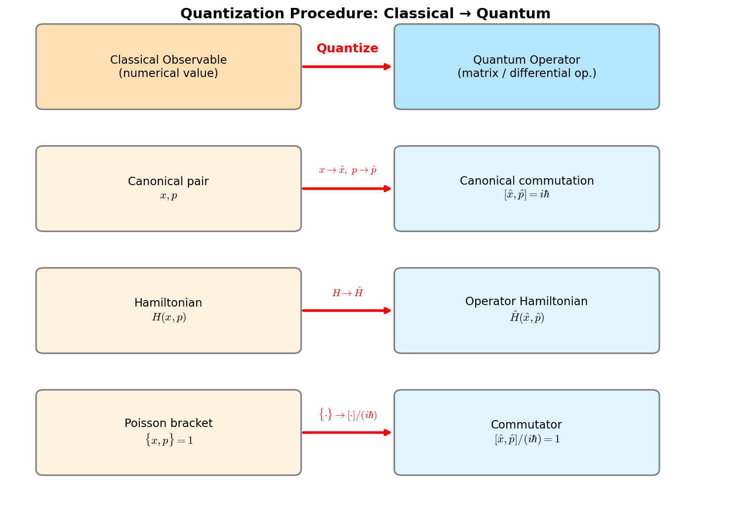
Fig. 7.2: The quantization procedure. Classical physical quantities (numerical values) are "promoted" to operators. Classical energy relation → operator equation (Schrödinger equation)—this correspondence is applied repeatedly to particles, fields, and strings.
⚪ Mei: I see—the form of the equation is determined just by "promoting" classical values to operators. Since the replacement rules are fixed, if the starting classical energy relation changes, the resulting equation changes too?
🟡 Lina: Yes. Conversely, once the starting point is determined, the equation is almost automatically determined—there's hardly any freedom of choice.
🟡 Lina: Yes. And through Born's probability interpretation, \(|\Psi(x, t)|^2\, dx\) gives the probability of finding the particle at position \(x \sim x+dx\) at time \(t\), with the integral over all space normalized to 1. For stationary states \(\Psi(x, t) = \psi(x)\, e^{-iEt/\hbar}\), the time-independent Schrödinger equation \(\hat{H}\psi = E\psi\) determines the energy eigenvalues \(E\).
🔵 Kai: "Replacing values with operators" is a pretty bold operation. Can it be used in other contexts too?
🟡 Lina: Good question. This procedure is called quantization. In fact, going forward, the same procedure is applied repeatedly—to fields in Ch. 8, and to strings in Ch. 14. Each time, a new world opens up.
🔵 Kai: So just by repeating the same procedure, the subject expands from "particle → field → string." But why this substitution works is... still fuzzy to me.
🟡 Lina: That fuzziness is legitimate. "Why it works" is justified after the fact by producing results consistent with experiment—that's the axiomatic character of quantum mechanics. As we proceed, the power of this procedure will become more apparent, so for now accept "this is the rule" and let's move forward.
🔵 Kai: I'll hold off on "why" and first see how far this rule can take us. ...But one thing bugs me—this substitution starts from the non-relativistic equation \(E = p^2/(2m) + V\), right? If we apply the same substitution to the relativistic energy relation \(E^2 = p^2c^2 + m^2c^4\), what happens?
🟡 Lina: Good intuition. The answer to that question is something we'll see at the end of this chapter.
📖 Important perspective: \(E \to i\hbar\,\partial_t\), \(p \to -i\hbar\,\partial_x\)—"promoting a classical energy equation to an operator equation"—this is the fundamental move of quantum mechanics. We'll use it repeatedly in subsequent sections.
✅ Comprehension Check: What is the procedure called quantization? What operator replacements are made for classical energy and momentum, respectively?
Answer
Quantization is the procedure of "promoting" classical physical quantities (numerical values) to operators. Specifically, one substitutes \(E \to i\hbar\,\partial_t\) and \(p \to -i\hbar\,\partial_x\). Applying this substitution to the classical energy relation \(E = p^2/(2m) + V\) yields the Schrödinger equation. This procedure is applied repeatedly in quantum field theory and string theory as well.
7.3 Summary of Key Points: Operators, Commutation Relations, and the Uncertainty Principle¶
🟡 Lina: When we replace position and momentum with the operators \(\hat{x} = x\) and \(\hat{p} = -i\hbar\,\partial/\partial x\), for any wave function we get
(the canonical commutation relation). The derivation is in Quantum Mechanics Ch. 8.
🔵 Kai: This means the order in which you multiply operators affects the result, right?
🟡 Lina: Yes. From this, the uncertainty principle is derived. Intuitively, when two operators don't commute, the "spread" of their measured values cannot both be made zero simultaneously. The mathematical formalization of this is Robertson's inequality. Let me clarify the notation before writing the equation. \(\langle \cdots \rangle\) denotes the expectation value—the average when you prepare the same state many times and repeat the same measurement. \(\Delta A\) is the spread (standard deviation) of measured values of quantity \(A\), defined as \(\Delta A = \sqrt{\langle \hat{A}^2 \rangle - \langle \hat{A} \rangle^2}\)—that is, you take the "mean of the squared values" minus the "square of the mean value" and take the square root. In high school statistics, you learned variance as \(\sigma^2 = \frac{1}{n}\sum(x_i - \bar{x})^2\); expanding this gives \(\overline{x^2} - \bar{x}^2\) ("mean of squares minus square of mean")—it's exactly the same structure. It represents how much the results scatter when you prepare the same state many times and measure \(A\). Using these, Robertson's inequality is written as
The right-hand side \(\langle [\hat{A}, \hat{B}] \rangle\) is the "expectation value (average) of the commutator"—how much the two operators fail to commute, averaged over the given state.
🔵 Kai: So the product of the spreads has a lower bound set by "how much they don't commute"?
🟡 Lina: Exactly. I'll defer the proof to Quantum Mechanics Ch. 8. What matters is the conclusion: as long as the commutator is nonzero, both spreads cannot simultaneously be zero. In particular, setting \(\hat{A} = \hat{x}\), \(\hat{B} = \hat{p}\) and substituting \([\hat{x}, \hat{p}] = i\hbar\), the right-hand side becomes \(\frac{1}{2}|\langle i\hbar \rangle| = \frac{1}{2}\hbar\) (since \(i\hbar\) is a constant, the expectation value in any state remains \(i\hbar\), and taking the absolute value gives \(\hbar\)), yielding
This is Heisenberg's uncertainty principle—I've visualized it in Fig. 7.3 "Visualization of the uncertainty principle", so look at the figure alongside the equations.
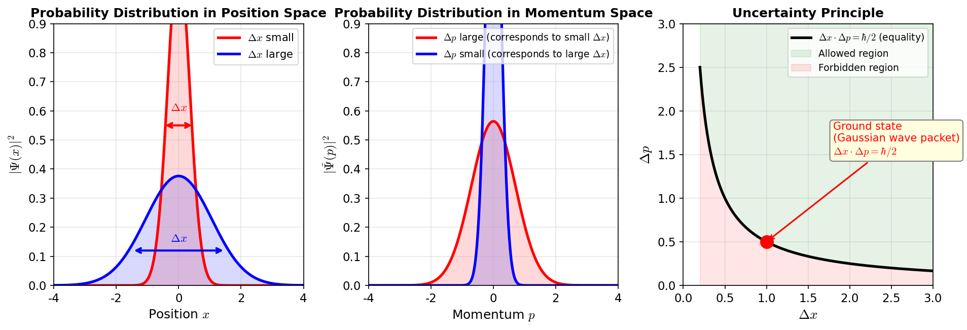
Fig. 7.3: Visualization of the uncertainty principle. Left: When the wave packet is narrow in position space (\(\Delta x\) small), it spreads in momentum space (\(\Delta p\) large). Center: The reverse is also true. Right: The equality \(\Delta x \cdot \Delta p = \hbar/2\) is satisfied by the ground state (Gaussian wave packet), and the region below this curve is physically forbidden.
🟡 Lina: And what's important is that this inequality is not about "measurement apparatus disturbing the particle." It's a consequence of the mathematical structure itself—that operators don't commute.
⚪ Mei: So even with an arbitrarily precise measurement apparatus, it cannot be circumvented—it's a constraint built into the skeleton of the theory, not a problem with instruments.
🟡 Lina: Exactly. And the uncertainty principle also provides the fundamental reason for the fact that Bohr postulated—"the electron doesn't fall into the nucleus." Confining an electron to a region of radius \(r\) means \(\Delta x \sim r\), so from the uncertainty principle \(\Delta x \cdot \Delta p \gtrsim \hbar\), we get \(\Delta p \sim \hbar/r\). The estimated kinetic energy becomes \(\langle T\rangle \sim (\Delta p)^2/(2m_e) \sim \hbar^2/(2m_er^2)\), which increases as \(r\) decreases. Meanwhile, the Coulomb potential is \(-e^2/(4\pi\varepsilon_0 r)\), which grows as \(1/r\)—slower than the \(1/r^2\) growth of the kinetic energy—so at some radius the kinetic energy increase wins. Minimizing the total energy yields \(r_{\min} \sim a_0\) (Quantum Mechanics 8.9 "Application: The Uncertainty Principle and Atomic Stability").
🔵 Kai: Oh, the more you confine it, the more it thrashes and tries to escape—the uncertainty principle acts as a wall that prevents collapse!
✅ Comprehension Check: Does the uncertainty principle mean "there's a limit to precision because the measurement apparatus disturbs the particle"? If not, what is its essence?
Answer
It is not a problem with measurement apparatus. The uncertainty principle is a consequence of the mathematical structure itself—that the position operator and momentum operator do not commute (\([\hat{x}, \hat{p}] = i\hbar\)). From the non-commutativity of operators, Robertson's inequality leads to \(\Delta x \cdot \Delta p \geq \hbar/2\), which is a fundamental constraint that cannot be circumvented by any measurement method.
🔵 Kai: So the Bohr radius comes out without Bohr's "angular momentum quantization" postulate! But why do the estimate from the uncertainty principle and the exact solution of the Schrödinger equation give exactly the same \(a_0\)? Is it coincidence?
🟡 Lina: It's not coincidence. The uncertainty principle estimate is the operation "minimize energy subject to \(\Delta x \cdot \Delta p \sim \hbar\)," and the exact Schrödinger equation solution is the operation "find the lowest eigenvalue of the Hamiltonian"—both start from the same physics (the canonical commutation relations of quantum mechanics) and find the same minimum energy state via different paths. So the agreement of the answers is inevitable.
🟡 Lina: And what connects directly to string theory is precisely this perspective: "commutation relations determine quantum structure." In Ch. 14, we quantize the string by imposing commutation relations isomorphic to \([\hat{a}, \hat{a}^\dagger] = 1\) on the vibrational modes of the string—the tools we prepare in the next section are directly used there.
📖 Foreshadowing string theory: The canonical commutation relation—"just one line of equation"—forms the skeleton of quantum mechanics, quantum field theory, and string theory alike. In the next section, we treat the harmonic oscillator as a concrete example.
7.4 The Harmonic Oscillator and Ladder Operators — The Most Important Preparation for String Theory¶
🟡 Lina: From here is the original content of this chapter. The algebraic solution of the harmonic oscillator is treated in detail in Quantum Mechanics Ch. 9, but since in string theory each vibrational mode of the string behaves as an independent harmonic oscillator, we need to have the ladder operator structure at hand. I'll walk through the derivation steps one by one, reaching all the way to the foreshadowing of string theory.
Rewriting the Hamiltonian¶
🟡 Lina: Quantizing the Hamiltonian of the harmonic oscillator—the total energy (kinetic energy + potential energy) expressed in terms of position and momentum—gives
The first term \(\hat{p}^2/(2m)\) corresponds to kinetic energy, and the second term \(m\omega^2\hat{x}^2/2\) to the spring's potential energy. This has the form of a sum of \(\hat{x}^2\) and \(\hat{p}^2\)—that is, a "sum of squares."
🔵 Kai: A sum of squares... for ordinary numbers, you can factor \(a^2 + b^2 = (a+ib)(a-ib)\), right? Can you do the same thing with operators? But operators don't commute, so it seems like it wouldn't be that simple...
🟡 Lina: Good eye. That "order matters" part is exactly the key. We try the same idea with operators. Can we express it as a product of "\(\hat{x} + (\text{something})\hat{p}\)" and "\(\hat{x} - (\text{something})\hat{p}\)"?—this is the motivation for ladder operators. Matching dimensions and coefficients gives
The symbol \(\dagger\) (dagger) denotes the operation called "Hermitian conjugate," but in the present context you can think of it simply as replacing \(i\) with \(-i\). Why this suffices: \(\hat{x}\) and \(\hat{p}\) are operators whose measured values are real (real-valued operators), so they don't change under \(\dagger\), and the prefactor \(\sqrt{m\omega/(2\hbar)}\) is also real and unchanged—so in the end only \(i\) changes to \(-i\). The general meaning of Hermitian conjugation is treated in Quantum Mechanics (Quantum Mechanics Ch. 8 onward), so for now just remember "\(\hat{a}\) and \(\hat{a}^\dagger\) are a pair differing only in the sign of \(i\)." However, since operators don't commute, \(\hat{a}^\dagger\hat{a}\) and \(\hat{a}\hat{a}^\dagger\) are not equal—let's compute that "discrepancy."
⚪ Mei: "Create a pair with opposite signs of \(i\)" and express the Hamiltonian as their product—the operator version of ordinary factoring.
🟡 Lina: Yes. Expanding \(\hat{a}\hat{a}^\dagger - \hat{a}^\dagger\hat{a}\) from the definitions, only the \(\hat{x}\hat{p} - \hat{p}\hat{x} = i\hbar\) terms survive:
Here the commutator obeys the distributive law \([A + B,\, C] = [A, C] + [B, C]\) and \([A,\, B + C] = [A, B] + [A, C]\) (which follow directly from the definition of operator products). Using this to expand into 4 terms:
The terms \([\hat{x}, \hat{x}] = 0\) and \([\hat{p}, \hat{p}] = 0\) vanish, leaving only the 2 terms containing \([\hat{x}, \hat{p}] = i\hbar\). Using the property that "constants can be pulled out of commutators"—\([A,\, cB] = c[A, B]\) (when \(c\) is a number):
Since \([\hat{p}, \hat{x}] = -[\hat{x}, \hat{p}] = -i\hbar\), the first term is \(\frac{-i}{m\omega}\cdot [\hat{x}, \hat{p}] = \frac{-i}{m\omega}\cdot i\hbar = \frac{\hbar}{m\omega}\), and the second term is \(\frac{i}{m\omega}\cdot [\hat{p}, \hat{x}] = \frac{i}{m\omega}\cdot(-i\hbar) = \frac{\hbar}{m\omega}\), giving together
Thus \([\hat{a}, \hat{a}^\dagger] = 1\) is proven.
🔵 Kai: Wow, after all that calculation, it cleanly reduces to \(= 1\) at the end!
🟡 Lina: Yes—that's the biggest payoff of defining the ladder operators. Using the number operator \(\hat{N} \equiv \hat{a}^\dagger\hat{a}\), the Hamiltonian is compressed to
reducing everything to just the eigenvalue problem of the number operator. You'll soon see why it's called the "number operator"—its eigenvalues turn out to be exactly the "counts" \(n = 0, 1, 2, \ldots\). The \(1/2\) offset is precisely the trace of operators not commuting—the origin of zero-point energy.
✅ Comprehension Check: By introducing ladder operators \(\hat{a}, \hat{a}^\dagger\), into what concise form is the harmonic oscillator Hamiltonian rewritten? What is the advantage of this rewriting?
Answer
It is rewritten as \(\hat{H} = \hbar\omega(\hat{N} + 1/2)\) (where \(\hat{N} = \hat{a}^\dagger\hat{a}\) is the number operator). The advantage is that the Hamiltonian, which was a quadratic form in \(\hat{x}\) and \(\hat{p}\), is consolidated into the eigenvalue problem of a single operator \(\hat{N}\). Once the eigenvalue \(n\) of \(\hat{N}\) is known, the energy is immediately determined as \(E_n = \hbar\omega(n + 1/2)\).
⚪ Mei: The \(\hat{H}\) that was a quadratic form in \(\hat{x}\) and \(\hat{p}\) has been folded into a form expressible with just a single operator \(\hat{N}\).
🟡 Lina: Yes. That's the point of beauty. Once you know the eigenvalue \(n\) of \(\hat{N}\), the energy is determined—this idea of "consolidating the eigenvalue problem into a single operator" will demonstrate its power when we quantize the string in Ch. 14.
The Energy Level Ladder¶
🟡 Lina: From \(\hat{H} = \hbar\omega(\hat{a}^\dagger\hat{a} + 1/2)\) and \([\hat{a}, \hat{a}^\dagger] = 1\), computing the commutation relation between \(\hat{H}\) and \(\hat{a}^\dagger\)—\([\hat{a}^\dagger\hat{a},\, \hat{a}^\dagger] = \hat{a}^\dagger\hat{a}\hat{a}^\dagger - \hat{a}^\dagger\hat{a}^\dagger\hat{a}\), and replacing \(\hat{a}\hat{a}^\dagger\) in the first term using the commutation relation \(\hat{a}\hat{a}^\dagger = \hat{a}^\dagger\hat{a} + 1\) gives \(\hat{a}^\dagger(\hat{a}^\dagger\hat{a} + 1) - \hat{a}^\dagger\hat{a}^\dagger\hat{a} = \hat{a}^\dagger\hat{a}^\dagger\hat{a} + \hat{a}^\dagger - \hat{a}^\dagger\hat{a}^\dagger\hat{a} = \hat{a}^\dagger\), so
⚪ Mei: From a single commutation relation, the structure "\(\hat{a}^\dagger\) raises energy by \(\hbar\omega\)" and "\(\hat{a}\) lowers it" emerges.
🟡 Lina: Let's see what this means. I'll use the notation \(|n\rangle\)—this represents "the state with energy quantum number \(n\)" (ket notation), referring to the same state as the wave function \(\psi_n(x)\). Writing \(\psi_n(x)\) makes you worry about the concrete form as a function of position \(x\), but what we want to do now is just the algebra of operators—"applying \(\hat{a}^\dagger\) raises energy by one level"—without using the specific value at position \(x\). So \(|n\rangle\), which specifies only "state \(n\)," is cleaner. When \(\hat{H}|n\rangle = E_n|n\rangle\), applying \(\hat{H}\) to \(\hat{a}^\dagger|n\rangle\)—using the commutator definition \([\hat{H}, \hat{a}^\dagger] = \hat{H}\hat{a}^\dagger - \hat{a}^\dagger\hat{H}\) rearranged as \(\hat{H}\hat{a}^\dagger = \hat{a}^\dagger\hat{H} + \hbar\omega\,\hat{a}^\dagger\):
So \(\hat{a}^\dagger|n\rangle\) is an eigenstate with energy \(E_n + \hbar\omega\). Similarly, \(\hat{a}|n\rangle\) is an eigenstate with energy \(E_n - \hbar\omega\).
🔵 Kai: \(\hat{a}^\dagger\) "raises by one level" and \(\hat{a}\) "lowers by one level"... but what happens if you keep lowering? Doesn't the energy go negative?
🟡 Lina: Good question. For the harmonic oscillator, both kinetic energy and potential are non-negative, so eigenvalues of \(\hat{H}\) must be \(\geq 0\)—if you keep lowering with \(\hat{a}\), you eventually reach a state that "can't be lowered further." That's the ground state satisfying \(\hat{a}|0\rangle = 0\) (the right side is the zero vector, meaning "there's no more state"). The energy of this state is
The \(n\)-th excited state, obtained by applying \(\hat{a}^\dagger\) to \(|0\rangle\) \(n\) times, has equally spaced energies:
I've drawn this equally-spaced ladder structure in Fig. 7.4 "Energy levels of the harmonic oscillator and ladder operators". Looking at the figure, even at the lowest level \(n = 0\), the energy isn't zero but retains \(\hbar\omega/2\)—that's the zero-point energy. Let's look at it in more detail next.
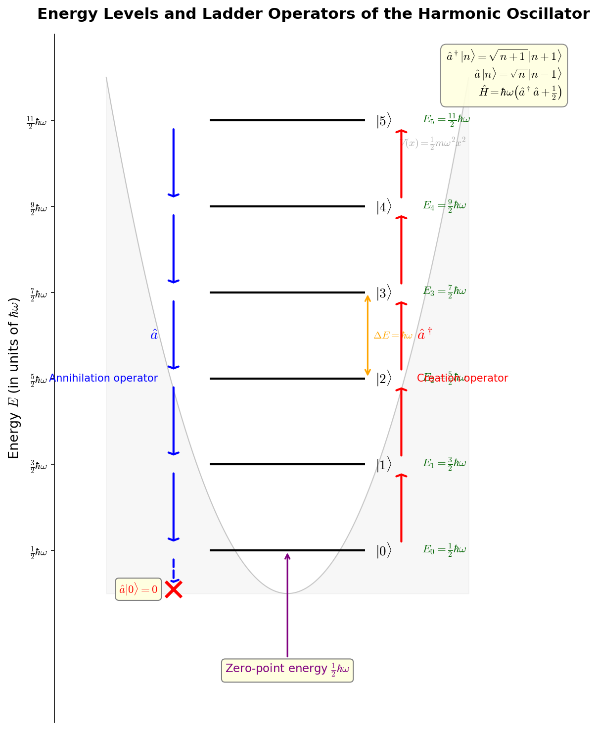
Fig. 7.4: Energy levels of the harmonic oscillator and ladder operators. The equally spaced energy levels \(E_n = \hbar\omega(n + 1/2)\) are drawn as a "ladder." \(\hat{a}^\dagger\) raises by one level and \(\hat{a}\) lowers by one level. Even in the ground state \(|0\rangle\), a zero-point energy of \(\hbar\omega/2\) remains.
⚪ Mei: The quantum number \(n\) is simultaneously "the label of the energy level" and "how many times \(\hat{a}^\dagger\) was applied." \(\hat{a}^\dagger\) raises by one level, \(\hat{a}\) lowers by one—this ladder structure is very easy to organize.
🔵 Kai: "Raise by one" and "lower by one" look like adding or removing something one at a time. If \(n\) is a "count of something," then \(\hat{a}^\dagger\) looks like it "adds one"... but one of what?
🟡 Lina: Good intuition. In fact, in the next chapter (quantum field theory), \(\hat{a}^\dagger\) and \(\hat{a}\) are reinterpreted as operators that "create" and "annihilate" one particle, respectively. \(n\) represents "the number of quanta"—this particle picture becomes the starting point of quantum field theory.
⚪ Mei: I see—right now \(n\) is "the label of the energy level," but in the next chapter it gets reinterpreted as "the number of particles." The operation of raising by one level with \(\hat{a}^\dagger\) corresponds to "creating one particle."
🔵 Kai: If it's "number of particles," that means we can handle situations where particles increase or decrease? That's a totally different world from the Schrödinger equation that tracks one particle's wave function... But wait—if particles are "born," what happens to energy conservation? You can't create something from nothing, right?
🟡 Lina: Good question. Energy conservation isn't violated—creating a particle requires energy commensurate with it. \(E = mc^2\) is precisely what tells us "how much is needed." For example, creating a particle-antiparticle pair of mass \(m\) requires at least \(2mc^2\) of energy supplied from outside. Energy is conserved while part of it is "converted" into mass. We'll revisit this in the last section, together with why a framework allowing particle number to change is necessary.
The Meaning of Zero-Point Energy \(\hbar\omega/2\)¶
🟡 Lina: The fact that even the ground state has \(E_0 = \hbar\omega/2 \neq 0\) is because a state with \(\Delta x = 0\), \(\Delta p = 0\) is forbidden by the uncertainty principle. In fact, in the ground state
—the equality holds, making it a minimum uncertainty state (Gaussian wave packet).
🔵 Kai: "Being unable to be completely at rest" is the essence of zero-point energy.
🟡 Lina: Yes. Moreover, this isn't a mathematical artifact—it's a real phenomenon confirmed by experiment, including helium's failure to solidify at atmospheric pressure, the Casimir effect, and molecular vibration spectra (details in Quantum Mechanics Ch. 9).
✅ Comprehension Check: What is the physical reason that the ground state energy of the harmonic oscillator is \(E_0 = \hbar\omega/2 \neq 0\) (zero-point energy)?
Answer
The uncertainty principle forbids simultaneously making position and momentum zero (\(\Delta x = 0\) and \(\Delta p = 0\)). The particle cannot be completely at rest, so even in the ground state it possesses a minimum amount of kinetic and potential energy. The ground state is a minimum uncertainty state (Gaussian wave packet) where the equality \(\Delta x \cdot \Delta p = \hbar/2\) holds.
Foreshadowing String Theory¶
🟡 Lina: Now for the part that connects directly to string theory. We'll treat it in detail in Ch. 14, but let me give you a preview. A string is a one-dimensional "thread," so describing its position requires two parameters—\(\tau\) representing the flow of time and \(\sigma\) representing position along the string (on a guitar string, the coordinate specifying somewhere from left end to right end). The spacetime coordinates of each point on the string are written \(X^\mu(\tau, \sigma)\). \(\mu\) labels the spacetime direction (\(\mu = 0\) for time, \(\mu = 1, 2, \ldots\) for space). Performing a Fourier expansion (expressing periodic vibration as a superposition of fundamental vibration, second harmonic, third harmonic, etc.) gives
(here we adopt the convention \(\sigma \in [0, 2\pi]\)). There are many symbols, but don't be intimidated—let's first grasp the big picture. The expression divides into two parts as shown by the braces above: the first half is "where the string as a whole is and how it moves (center-of-mass motion)," the second half is "vibrations on the string." In the vibration part, \(\alpha_n^\mu\) is the amplitude of the right-moving wave on the string, and \(\tilde{\alpha}_n^\mu\) (with tilde) is the amplitude of the left-moving wave—two kinds of waves exist independently. For now, it's enough to remember the structure: "the string's vibrations are described by a collection of Fourier coefficients \(\alpha_n^\mu\) (right-moving) and \(\tilde{\alpha}_n^\mu\) (left-moving)." The reason the sum \(\sum_{n \neq 0}\) includes negative \(n\), and details like the reality condition \(\alpha_{-n}^\mu = (\alpha_n^\mu)^*\), will be treated in Ch. 14.
🔵 Kai: The formula is big, but I can see it splits into "center of mass + vibrations." Could you explain each symbol in a bit more detail?
🟡 Lina: Of course. First, \(x_0^\mu\) is the center-of-mass position and \(p_0^\mu\) is the center-of-mass momentum—the part describing where the string as a whole is in space and which direction it's moving. The \(2\alpha'\) in \(2\alpha' p_0^\mu\tau\) is a "coefficient converting momentum to velocity"—what was \(1/m\) in particle mechanics \(x = x_0 + (p/m)t\) gets replaced by \(2\alpha'\) for the string (because tension replaces mass). \(\alpha'\) (alpha-prime) is a new parameter defined using the string tension \(T\) (introduced in Ch. 6) as \(\alpha' = 1/(2\pi T)\)—the more tightly the string is strung, the smaller \(\alpha'\) becomes. Since \(\sqrt{\alpha'}\) corresponds to the string length scale \(\ell_s\) (the typical size of the string), \(\alpha'\) is also the constant determining "how big the string is." For now, just think of it as "a constant representing the stiffness = size of the string."
🔵 Kai: Got it—\(x_0\) and \(p_0\) are center-of-mass position and momentum, \(\alpha'\) is the string's stiffness. So what about \(\tau\) and \(\sigma\)?
🟡 Lina: Picture a guitar string—\(\tau\) is the flow of time (the time coordinate on the two-dimensional surface the string sweeps out over time—called the worldsheet), and \(\sigma\) is position along the string (the coordinate from left end to right end). In addition to the center-of-mass motion (the \(x_0^\mu + p_0^\mu\tau\) part), the vibrations happening on the string are expressed as a superposition of waves (Fourier series). \(n = 1\) is the fundamental vibration, \(n = 2\) is the second harmonic, and so on. \(e^{-in(\tau - \sigma)}\) corresponds to a right-moving wave on the string, and \(e^{-in(\tau + \sigma)}\) to a left-moving wave. Recall from high school physics that \(\sin(\omega t - kx)\) is a rightward traveling wave—when \(t\) and \(x\) combine with opposite signs, the wave profile moves in the positive \(x\) direction as time advances. By the same reasoning, the combination \(\tau - \sigma\) represents a wave moving in the positive \(\sigma\) direction (rightward) (\(e^{i\theta} = \cos\theta + i\sin\theta\) by Euler's formula, so the complex exponential is a convenient way to write combinations of \(\cos\) and \(\sin\) representing oscillations/waves). Vibrations on a guitar string also propagate in both directions, right? So the first half \(x_0^\mu + p_0^\mu\tau\) is "translational motion of the entire string," the \(\sum\) in the second half is "vibrations on the string," and the vibrations split into right-movers \(\alpha_n^\mu\) and left-movers \(\tilde{\alpha}_n^\mu\)—that's the structure.
⚪ Mei: I see—center-of-mass motion and vibrations are cleanly separated, and the vibration part further splits independently into right-movers and left-movers—a very organized structure.
🟡 Lina: Yes. And here's the important point—this is still just classical Fourier coefficients, but when we apply the "promote to operators" procedure we just learned, what do you think happens to this independence? In fact, the structure "classically independent" is preserved even after quantization. Up to now, \(\alpha_n^\mu\) (right-moving wave amplitude) and \(\tilde{\alpha}_n^\mu\) (left-moving wave amplitude) are classical Fourier coefficients—just numerical values. Applying the quantization procedure learned in the previous section (the same spirit as \(E \to i\hbar\,\partial_t\), \(p \to -i\hbar\,\partial_x\)—the operation of promoting classical quantities to operators), the \(\alpha_n^\mu\) are "promoted" to operators satisfying commutation relations of essentially the same structure as \(\hat{a}, \hat{a}^\dagger\) we just learned:
(for positive integers \(m, n > 0\)). The \(m\) on the right-hand side is not mass—it's the same mode number as the subscript \(m\) on the left.
🔵 Kai: The mode number \(m\) appears directly on the right side. It's a bit different from the harmonic oscillator's \([\hat{a}, \hat{a}^\dagger] = 1\)...
🟡 Lina: Good observation. Let's check with a concrete example: if \(m = n = 3\), the right side is \(3\,\eta^{\mu\nu}\); if \(m = 2,\, n = 5\), then \(\delta_{25} = 0\) so the right side is zero. That is, thanks to \(\delta_{mn}\), modes with \(m \neq n\) have zero commutation relation (mutually independent), and only when \(m = n\) does the right side become \(m\,\eta^{\mu\nu}\). This extra \(m\) reflects the \(1/n\) factor multiplying each mode's coefficient in the Fourier expansion—meaning \(\alpha_n^\mu\) is the raw, "unnormalized" Fourier coefficient. If we immediately redefine \(\hat{a}_n^\mu \equiv \alpha_n^\mu/\sqrt{n}\), the \(m\) disappears and we recover the same form as the harmonic oscillator. Here \(\alpha_n^{\mu\dagger} \equiv \alpha_{-n}^\mu\) is defined—so the operator \(\alpha_n^\mu\) for positive \(n\) is the "annihilation" side, and \(\alpha_{-n}^\mu = \alpha_n^{\mu\dagger}\) corresponding to negative \(-n\) is the "creation" side. Here \(\alpha_n^{\mu\dagger}\) is the Hermitian conjugate of \(\alpha_n^\mu\)—in the Fourier expansion, if the coefficient \(\alpha_n^\mu\) for \(n > 0\) is the operator that "lowers (annihilates) a wave by one level," then \(\alpha_n^{\mu\dagger}\) is its partner that "excites (creates) by one level" (the same relationship as \(\hat{a}\) and \(\hat{a}^\dagger\) for the harmonic oscillator). Redefining \(\hat{a}_n^\mu \equiv \alpha_n^\mu/\sqrt{n}\) (\(n > 0\)), the commutation relation becomes
Let's verify: substituting \(\alpha_m^\mu = \sqrt{m}\,\hat{a}_m^\mu\) into the original commutation relation gives \(\sqrt{m}\cdot\sqrt{n}\,[\hat{a}_m^\mu, \hat{a}_n^{\nu\dagger}] = m\,\delta_{mn}\,\eta^{\mu\nu}\). Dividing both sides by \(\sqrt{m}\cdot\sqrt{n}\) gives \([\hat{a}_m^\mu, \hat{a}_n^{\nu\dagger}] = \frac{m}{\sqrt{mn}}\,\delta_{mn}\,\eta^{\mu\nu}\); since \(\delta_{mn}\) is multiplied on the right, when \(m \neq n\) the entire right side is zero—so we only need to consider \(m = n\). When \(m = n\), \(\sqrt{mn} = \sqrt{m \cdot m} = m\) so \(\frac{m}{\sqrt{mn}} = \frac{m}{m} = 1\). Thus \([\hat{a}_m^\mu, \hat{a}_n^{\nu\dagger}] = \delta_{mn}\,\eta^{\mu\nu}\) is obtained—the mode number coefficient cancels cleanly.
⚪ Mei: With a single redefinition the extra \(m\) vanishes, reducing to exactly the same form as the harmonic oscillator. Satisfying.
🟡 Lina: For the same spatial directions (\(\mu = \nu = i\)), \(\eta^{ii} = +1\), confirming isomorphism with the harmonic oscillator's \([\hat{a}, \hat{a}^\dagger] = 1\)—meaning each mode behaves as an independent harmonic oscillator. Here \(\delta_{mn}\) is the Kronecker delta (\(1\) when \(m = n\), \(0\) when \(m \neq n\)), and \(\eta^{\mu\nu}\) is the Minkowski metric from Ch. 5 (\(\eta^{\mu\nu} = \mathrm{diag}(-1, +1, +1, +1)\)). For spatial components (\(\mu = \nu = i\)), \(\eta^{ii} = +1\) gives the same positive sign as the harmonic oscillator's \([\hat{a}, \hat{a}^\dagger] = 1\). On the other hand, for the time component \(\eta^{00} = -1\) and the sign flips—this "negative norm state" problem is addressed in Ch. 14.
🔵 Kai: If each mode becomes an independent harmonic oscillator, does that mean pairs of \(\hat{a}, \hat{a}^\dagger\) appear for as many modes as there are?
🟡 Lina: Exactly. That is, quantizing the string = simultaneously quantizing infinitely many harmonic oscillators. For each mode number \(n = 1, 2, 3, \ldots\) and each spacetime direction \(\mu\), one pair "\(\hat{a}, \hat{a}^\dagger\)" emerges. Recall the vibrations of a guitar string—I've drawn from the fundamental vibration to higher vibrational modes in Fig. 7.5 "Vibrational modes of the string and Fourier expansion", so use it to build your intuition.
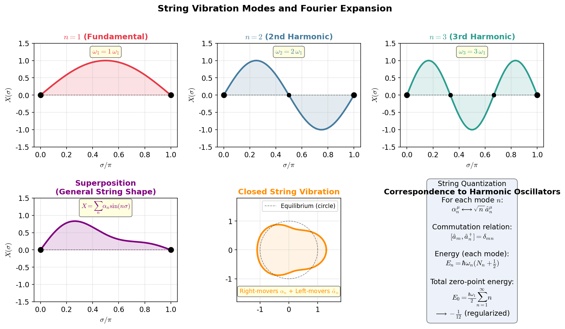
Fig. 7.5: Vibrational modes of the string and Fourier expansion. Top row: fundamental vibration \((n=1)\), second harmonic \((n=2)\), third harmonic \((n=3)\). Bottom left: a general string shape is a superposition of these. Bottom center: vibrations of a closed string (right-moving waves \(\alpha_n\) + left-moving waves \(\tilde{\alpha}_n\)). Bottom right: summary showing that quantization of each mode is isomorphic to the harmonic oscillator \([\hat{a}, \hat{a}^\dagger] = 1\).
✅ Comprehension Check: State in one sentence the relationship between string quantization and the harmonic oscillator. Why is it necessary to carefully study a single harmonic oscillator in this chapter?
Answer
Quantizing the string is equivalent to "simultaneously quantizing infinitely many harmonic oscillators." When the string's position is Fourier expanded, the coefficient of each vibrational mode behaves as an independent harmonic oscillator, each satisfying commutation relations isomorphic to \([\hat{a}, \hat{a}^\dagger] = 1\). Therefore, understanding the ladder operator structure of a single harmonic oscillator means that structure is used repeatedly—as many times as there are modes—in string theory.
⚪ Mei: So the structure of the single harmonic oscillator we're studying now is used repeatedly, as-is, in string theory.
🟡 Lina: Exactly. And the zero-point energy of the string is the sum of \(\hbar\omega_n/2\) from each mode:
For the string, just as with a guitar string, the frequencies are integer multiples of the fundamental \(\omega_n = n\,\omega_1\), so this becomes
—a divergent sum.
🔵 Kai: If infinity appears, doesn't it become physically meaningless...?
🟡 Lina: A natural question. Actually, summing \(1 + 2 + 3 + \cdots\) directly diverges, but using a mathematical prescription called zeta function regularization, one can consistently assign the finite value \(-1/12\) to this sum. The "zeta function" is the function \(\zeta(s) = \sum_{n=1}^\infty 1/n^s\) studied by mathematician Riemann (an infinite series converging for \(s > 1\)); formally "extending" it to \(s = -1\) gives \(\sum n = \zeta(-1) = -1/12\)—that's the origin of the name.
🔵 Kai: \(1 + 2 + 3 + \cdots = -1/12\)...!? Can we really trust that?
🟡 Lina: It does go against intuition. But while "replacing a divergent sum with a finite value" sounds like a magic trick, results obtained through this prescription are consistent with experiment and the internal consistency of the theory—so it's trusted as a physically meaningful procedure. The detailed mechanism is treated in Ch. 14, so for now just remember that "there exists a method to control the infinite sum of zero-point energies." And because this prescription works consistently, the stunning result critical dimension \(D = 26\) (bosonic string) is determined. The zero-point energy studied in this chapter directly connects to one of the deepest results in string theory. @exercise: Divergent sum of zero-point energies and critical dimension \(D = 26\) → Problem A-2. Divergent Sum of Zero-Point Energy and the Critical Dimension D = 26
🟡 Lina: And writing the excitation number of each mode \(n\) as \(N_n\), the state of the entire string is completely specified by the list "how many levels each mode is excited to" \(\{N_1, N_2, N_3, \ldots\}\). The perspective of reading \(N_n\) as "the number of quanta in mode \(n\)" is called the occupation number representation—specifying the state by how many quanta are in each mode. This occupation number representation demonstrates its true value in both the next chapter (quantum field theory) and string theory.
⚪ Mei: I see—since each mode is independent, the entire string state is determined just by listing the quantum numbers \(N_n\) per mode—a very easy-to-organize structure.
Table 7.2: Objects of quantization and the reappearance of "harmonic oscillator structure"
| Object | Commutation relation | Meaning of quantum number | Chapter |
|---|---|---|---|
| 1D harmonic oscillator | \([\hat{a}, \hat{a}^\dagger] = 1\) | \(n\) = energy level | This chapter |
| Free scalar field | \([\hat{a}_{\vec{k}}, \hat{a}_{\vec{k}'}^\dagger] = \delta(\vec{k}-\vec{k}')\) | \(n_{\vec{k}}\) = number of particles with momentum \(\vec{k}\) | Ch. 8 |
| String vibrational modes | \([\hat{a}_m^\mu, \hat{a}_n^{\nu\dagger}] = \delta_{mn}\eta^{\mu\nu}\) | \(N_n\) = excitation number of mode \(n\) | Ch. 14 |
The ladder operator pattern recurring throughout this chapter
- Derive \([\hat{a}, \hat{a}^\dagger] = 1\) from the canonical commutation relation \([\hat{x}, \hat{p}] = i\hbar\)
- The Hamiltonian is compressed to \(\hat{H} = \hbar\omega(\hat{a}^\dagger\hat{a} + 1/2)\)
- \(\hat{a}^\dagger\) and \(\hat{a}\) raise and lower energy one step at a time
- From the existence of a lowest energy state, quantum numbers \(n = 0, 1, 2, \ldots\) emerge naturally
- The ground state zero-point energy is a direct consequence of the uncertainty principle
This pattern is repeated in varying forms in Ch. 8 (field quantization), Ch. 14 (string quantization), and Ch. 17 (fermionic extension of the superstring). This is what we want to firmly establish here.
7.5 Summary of Key Points: Spin¶
🟡 Lina: Independent of motion in position space, particles possess spin—an intrinsic angular momentum. It's not classical rotation but a purely quantum mechanical degree of freedom.
🔵 Kai: The name says "rotation" but it's different from spinning?
🟡 Lina: Since the model treating electrons as "point particles" works best, a point "spinning" makes no sense. In the Stern-Gerlach experiment, a beam of silver atoms passing through a magnetic field splits into exactly 2 beams—if it were continuous rotation, it should spread into a fan shape, but only discrete values are allowed. It's a purely quantum mechanical degree of freedom that classical rotation cannot explain—that's what kind of thing it is. Details are in Quantum Mechanics Ch. 5 Introduction via the Stern-Gerlach experiment, Quantum Mechanics Ch. 17 Formulation using Pauli matrices, and Quantum Mechanics Ch. 18 Identical particles and statistics. Summarizing only the conclusions needed for Part III:
Table 7.3: Summary of basic spin properties
| Item | Content |
|---|---|
| Spin quantum number \(s\) | Takes values \(0, \tfrac{1}{2}, 1, \tfrac{3}{2}, 2, \ldots\) |
| Spin \(z\)-component | \(S_z = \hbar m_s\), with \(m_s = -s, -s+1, \ldots, s\) (\(2s+1\) values) |
| Commutation relations | \([\hat{S}_i, \hat{S}_j] = i\hbar\,\epsilon_{ijk}\,\hat{S}_k\) (see note below; isomorphic to orbital angular momentum) |
| Bosons (integer \(s\)) | Any number can occupy the same state. Photon (\(s = 1\)), graviton (\(s = 2\)), Higgs (\(s = 0\)) |
| Fermions (half-integer \(s\)) | Only 1 per state (Pauli exclusion principle). Electron, quark (\(s = 1/2\)) |
Meaning of \(\epsilon_{ijk}\) (totally antisymmetric symbol): The indices \(1, 2, 3\) correspond to the \(x, y, z\) directions respectively. \((i,j,k) = (1,2,3), (2,3,1), (3,1,2)\) gives \(+1\); \((1,3,2), (3,2,1), (2,1,3)\) gives \(-1\); repeated indices give \(0\). In other words, cyclic shifts of \((1,2,3)\) give \(+1\), swapping adjacent indices gives \(-1\). Example: \([\hat{S}_x, \hat{S}_y] = i\hbar\,\hat{S}_z\), \([\hat{S}_y, \hat{S}_x] = -i\hbar\,\hat{S}_z\).
⚪ Mei: "Why integer spin corresponds to bosons and half-integer spin to fermions"—that reason hasn't been explained yet, has it?
🟡 Lina: Right. This is first proven by the spin-statistics theorem of quantum field theory (Quantum Mechanics Ch. 18 or Quantum Field Theory Quantum Field Theory Ch. 5). For now, just accept the result. The distinction between bosons and fermions is the most important classification axis that appears repeatedly in this book. For example—
- Ch. 9 Particle classification in the Standard Model (bosons mediating forces / fermions making up matter)
- Ch. 15 Spectrum of the bosonic string (containing the graviton)
- Ch. 17 Superstring theory (extension to include fermions)
In all cases, "integer spin vs. half-integer spin" determines the skeletal internal structure. We'll leave the details of spin to Quantum Mechanics; for this book, keeping just the classification in Table 7.3 "Summary of basic spin properties" at hand is sufficient.
✅ Comprehension Check: Explain the difference between bosons and fermions from the perspective of spin quantum number and occupancy of identical states.
Answer
Bosons are particles with integer spin quantum number \(s\) (\(0, 1, 2, \ldots\)) that can occupy the same quantum state in any number (e.g., photons, gravitons). Fermions are particles with half-integer spin quantum number (\(1/2, 3/2, \ldots\)) that, by Pauli's exclusion principle, allow only one per quantum state (e.g., electrons, quarks). This distinction is proven by the spin-statistics theorem of quantum field theory.
7.6 The Remaining Question — The Collision Between Relativity and Quantum Theory¶
🟡 Lina: Quantum mechanics explains the microscopic world—atoms, molecules, chemical bonds, semiconductors, superfluidity—with astonishing precision. But it has one decisive flaw.
🔵 Kai: A flaw...? Even though it's that powerful?
🟡 Lina: It's incompatible with special relativity.
🔵 Kai: Wait, where is it incompatible?
🟡 Lina: Look at the time-dependent Schrödinger equation one more time:
The left side has a first-order time derivative; the spatial part on the right has a second-order derivative. As we confirmed in Ch. 5, special relativity demands that time and space be treated on equal footing through the Minkowski metric \(\eta_{\mu\nu}\). Therefore this equation changes form under Lorentz transformations—it is not relativistically covariant.
🔵 Kai: The derivative orders don't match on left and right.
Table 7.4: Incompatibility of the Schrödinger equation with special relativity
| Item | Schrödinger equation | Requirement of special relativity |
|---|---|---|
| Time derivative | 1st order (\(\partial/\partial t\)) | Treat time and space equally |
| Spatial derivative | 2nd order (\(\partial^2/\partial x^2\)) | Treat time and space equally |
| Lorentz transformation | Form changes (not covariant) | Requires form invariance |
| Energy relation | \(E = p^2/(2m) + V\) (non-relativistic) | \(E^2 = p^2c^2 + m^2c^4\) |
| Particle number | Fixed (assumed conserved) | Pair creation possible via \(E = mc^2\) |
🟡 Lina: Exactly. This structural flaw produces two serious consequences when one tries to force compatibility with relativity:
- Appearance of negative energy solutions — The square root of the relativistic energy-momentum relation \(E^2 = p^2c^2 + m^2c^4\) has an \(E < 0\) branch. Dirac interpreted this as antiparticles.
- Non-conservation of particle number — If energy exceeding \(E = mc^2\) is available, particle-antiparticle pairs can be created from the vacuum. The Schrödinger equation with fixed particle number cannot describe this.
⚪ Mei: So because relativity teaches "equivalence of energy and mass," particles can be born—yet the framework of quantum mechanics cannot handle processes where particle number changes—a fundamental incompatibility.
🔵 Kai: If particles increase and decrease, the method of tracking "one particle's wave function" like the Schrödinger equation won't work. So what do we track as the fundamental object?
🟡 Lina: Exactly. To reconcile relativity and quantum mechanics, we need a new framework that allows "particle number to change." That framework is quantum field theory, treated in Ch. 8. We promote the field itself to an operator and describe particles as excitations of the field. The \(\hat{a}^\dagger\) (creation operator) and \(\hat{a}\) (annihilation operator) learned in this chapter directly become the tools describing particle creation and annihilation—this correspondence is beautiful.
✅ Comprehension Check: What is the structural reason the Schrödinger equation is incompatible with special relativity? What two physical consequences arise from this?
Answer
The Schrödinger equation has a first-order time derivative and a second-order spatial derivative, so it changes form under Lorentz transformations that treat time and space equally. The consequences of this incompatibility are: (1) The square root of the relativistic energy-momentum relation produces negative energy solutions, requiring the existence of antiparticles. (2) Particle-antiparticle pairs are created at energies above \(E = mc^2\), so particle number is not conserved and cannot be described within a framework that tracks single-particle wave functions.
%%{init: {"theme": "default", "themeCSS": ".edgePath .path, .flowchart-link { stroke-width: 2px !important; }"}}%%
flowchart TD
    A["Schrödinger equation<br/>∂/∂t is 1st order, ∂²/∂x² is 2nd order"]
    B["Not Lorentz invariant"]
    C["Relativistic wave equations<br/>(Klein-Gordon, Dirac)"]
    D["Negative energy solutions<br/>→ antiparticles"]
    E["Non-conservation of particle number<br/>→ pair creation/annihilation"]
    F["Quantum field theory (Chapter 8)"]
    G["String theory (Chapter 13 onward)"]

    A --> B
    B --> C
    C --> D
    C --> E
    D --> F
    E --> F
    F --> G
Fig. 7.6: Path from the Schrödinger equation to quantum field theory and string theory
🔵 Kai: So the trunks of relativity and quantum theory collide head-on here for the first time. But "promoting the field itself to an operator"—that means doing a substitution like \(E \to i\hbar\,\partial_t\), but now for the field? Since a field has a value at each point in space, does that mean the object being substituted is infinite in number...?
🟡 Lina: Exactly. At each point in space there are quantities corresponding to "position and momentum," and commutation relations are imposed on each—so you're quantizing infinitely many degrees of freedom at once. And from that collision, the field picture transcending the particle picture is born, and beyond that the string picture awaits—this is the story of the latter half of this book.
📖 Connection to Quantum Mechanics: The Klein-Gordon equation, the Dirac equation, and Dirac's sea interpretation are treated in Quantum Mechanics Ch. 27. In Part III of this book, we reconstruct these in the next chapter from the angle of "the necessity of a theory with variable particle number = quantum field theory."
Preview of Next Chapter¶
The Schrödinger equation changes form under Lorentz transformations. The trunk of relativity (Chapters 5–6) and the trunk of quantum theory (this chapter) finally collide head-on here. In Ch. 8 title, we venture into the bold idea of promoting the field itself to an operator—quantum field theory—and build the framework to describe pair creation and annihilation. Let us witness the moment when the ladder operators \(\hat{a}, \hat{a}^\dagger\) acquired in this chapter are reinterpreted as particle annihilation and creation operators.
Exercises¶
📝 Exercises:
- Divergent sum of zero-point energies and critical dimension \(D = 26\) → Problem A-2. Divergent Sum of Zero-Point Energy and the Critical Dimension D = 26
References¶
- Quantum Mechanics Ch. 1 The 3 crises of classical physics and the Bohr model
- Quantum Mechanics Ch. 7 Wave function and Schrödinger equation
- Quantum Mechanics Ch. 8 Commutation relations, uncertainty principle, and atomic stability
- Quantum Mechanics Ch. 9 Stationary problems in 1D and algebraic solution of the harmonic oscillator
- Quantum Mechanics Ch. 15 Angular momentum algebra—generalization of ladder operators
- Quantum Mechanics Ch. 5, Quantum Mechanics Ch. 17, Quantum Mechanics Ch. 18 Spin
- Quantum Mechanics Ch. 27 Klein-Gordon and Dirac equations and the negative energy problem
- David Tong, Lectures on Quantum Field Theory, Ch.1 (Why quantum mechanics alone is insufficient)
- Carlo Rovelli, Reality Is Not What It Seems, Ch.6–7 (The birth and completion of quantum mechanics)
Feedback on this page
Let us know if something was unclear, incorrect, or could be improved.