Appendix B: Foundations of Linear Algebra and Hilbert Spaces
Story so far:
In Appendix A, we organized the fundamentals of complex numbers essential to quantum mechanics—arithmetic operations, polar form, Euler's formula, complex conjugation, and more. In this Appendix, we build the world of vectors and matrices whose "components" are complex numbers—linear algebra—and connect it to Hilbert spaces, the stage on which quantum mechanics is set.
Goals of this Appendix:
- Understand linear algebra, the mathematical language of quantum mechanics, as a natural extension of high school "vectors" and "matrices"
- Cover vector spaces, inner products, orthonormal bases, linear operators, eigenvalue problems, Hermitian matrices, unitary matrices, and tensor products, and grasp what changes when extending to infinite-dimensional Hilbert spaces
- These constitute the "grammar" of quantum mechanics—states, observables, time evolution, and composite systems are all described using the tools developed here
B.1 Vector Spaces—Anything That Allows "Addition" and "Scalar Multiplication" Is a Vector
🟡 Lina: In high school, vectors were "arrows." But in quantum mechanics, we use vectors in a much broader sense. Let me define "what a vector space is" as concretely as possible.
🔵 Kai: What do you mean by vectors that aren't arrows?
🟡 Lina: Good question. The bottom line is that anything that supports "addition" and "scalar multiplication" and satisfies several natural rules can be called a vector. Arrows qualify, ordered tuples of numbers qualify, and in fact, functions can be vectors too.
🟡 Lina: To be precise, a set \(V\) is a vector space if, for any elements (called vectors) \(\mathbf{u}, \mathbf{v}, \mathbf{w}\) of \(V\) and scalars \(c, c_1, c_2\) (real or complex numbers), the following 8 axioms are satisfied.
Table B.1: The 8 axioms of a vector space
| No. | Axiom | Meaning |
|---|---|---|
| 1 | \(\mathbf{u} + \mathbf{v} \in V\) | The result of addition stays in \(V\) (closure) |
| 2 | \(\mathbf{u} + \mathbf{v} = \mathbf{v} + \mathbf{u}\) | Order of addition can be swapped |
| 3 | \((\mathbf{u} + \mathbf{v}) + \mathbf{w} = \mathbf{u} + (\mathbf{v} + \mathbf{w})\) | Associativity of addition |
| 4 | \(\exists\, \mathbf{0}:\ \mathbf{u} + \mathbf{0} = \mathbf{u}\) | A zero vector exists |
| 5 | \(\exists\, (-\mathbf{u}):\ \mathbf{u} + (-\mathbf{u}) = \mathbf{0}\) | An additive inverse exists |
| 6 | \(c\mathbf{u} \in V\) | The result of scalar multiplication stays in \(V\) |
| 7 | \(c_1(c_2 \mathbf{u}) = (c_1 c_2)\mathbf{u}\), \(1 \cdot \mathbf{u} = \mathbf{u}\) | Associativity of scalar multiplication and scalar identity |
| 8 | \(c_1(\mathbf{u}+\mathbf{v}) = c_1\mathbf{u} + c_1\mathbf{v}\), \((c_1+c_2)\mathbf{u} = c_1\mathbf{u} + c_2\mathbf{u}\) | Distributive laws (two of them) |
🔵 Kai: Whoa, there are 8 of them?
⚪ Mei: But looking at each one individually, they're all things that were obvious for high school vectors. "You can swap the order of addition," "there's a zero vector," and so on.
🟡 Lina: Exactly. We're just making the obvious explicit. But the key point is that anything satisfying these axioms can be called a vector space. When the scalars are complex numbers \(\mathbb{C}\), we specifically call it a complex vector space. That's what we use in quantum mechanics.
🟡 Lina: Let me give three concrete examples.
Example 1: \(N\) complex numbers arranged in a column—\(\mathbb{C}^N\)
Addition is component-wise, scalar multiplication is component-wise. A natural extension of high school vectors.
Example 2: The case \(N = 2\)—\(\mathbb{C}^2\)
This appears as the state space for spin-1/2 in Ch. 5. It's 2-dimensional, but since the components are complex numbers, the effective "degrees of freedom" are 4.
🔵 Kai: Huh, just 2 components but 4 degrees of freedom.
🟡 Lina: Example 3: The set of square-integrable functions—\(L^2\)
"Square-integrable" means that when you integrate \(|f(x)|^2\) from \(-\infty\) to \(+\infty\), you get a finite value—in other words, the function approaches zero sufficiently rapidly at infinity. For example, \(f(x) = e^{-x^2}\) rapidly approaches zero at infinity, so it belongs to \(L^2\). On the other hand, \(f(x) = \sin x\) keeps oscillating at infinity. \(|\sin x|^2 = \sin^2 x\) takes values between 0 and 1 indefinitely, so as you extend the integration interval, the area accumulates without bound. More quantitatively, using \(\sin^2 x = (1 - \cos 2x)/2\) derived from the double-angle formula, we get \(\int_0^{2\pi} \sin^2 x\, dx = \pi\), so an area of \(\pi\) is added per period. This contribution repeats endlessly, so \(\int_{-\infty}^{\infty} |\sin x|^2\, dx = \infty\), and it doesn't belong to \(L^2\). With function addition \((f+g)(x) = f(x) + g(x)\) and scalar multiplication \((cf)(x) = c\,f(x)\), the 8 axioms are satisfied. Let me verify "closure under addition" in particular—that is, if \(f, g \in L^2\) then \(f + g \in L^2\).
The key is the following inequality:
Let me show the derivation in 3 steps.
Step 1 (Triangle inequality): Since the function values \(f(x)\) and \(g(x)\) at each point \(x\) are complex numbers, the triangle inequality for complex numbers \(|f(x)+g(x)| \leq |f(x)| + |g(x)|\) holds. This is the geometric property that "when adding two complex numbers as arrows, the roundabout length \(|f(x)| + |g(x)|\) is at least as large as the direct length \(|f(x)+g(x)|\)." Below, I'll omit that these are inequalities at each point \(x\) and write \(|f+g| \leq |f| + |g|\).
Step 2 (Squaring): Squaring both sides gives \(|f+g|^2 \leq (|f|+|g|)^2 = |f|^2 + 2|f||g| + |g|^2\).
Step 3 (Bounding the cross term): We use \(2|f||g| \leq |f|^2 + |g|^2\). This follows immediately from expanding \((|f|-|g|)^2 \geq 0\) to get \(|f|^2 - 2|f||g| + |g|^2 \geq 0\).
⚪ Mei: Just expanding \((|f|-|g|)^2 \geq 0\) gives the bound on the cross term. Simple.
🟡 Lina: Combining Steps 2 and 3 gives \(|f+g|^2 \leq 2(|f|^2 + |g|^2)\). Integrating both sides:
This shows \(f+g \in L^2\). This is the space where wave functions live.
🔵 Kai: Functions are vectors!?
🟡 Lina: Yes. They support "addition" and "scalar multiplication" and satisfy the axioms, so they form a perfectly valid vector space. However, there's a major difference: \(\mathbb{C}^N\) is finite-dimensional, while \(L^2\) is infinite-dimensional. In this Appendix, we'll mainly work in finite dimensions and summarize what changes in infinite dimensions at the end.
✅ Comprehension Check: Why can the set of functions \(L^2\) be regarded as a vector space?
Answer
Because function addition \((f+g)(x) = f(x) + g(x)\) and scalar multiplication \((cf)(x) = c\,f(x)\) are defined, and they satisfy the 8 axioms of a vector space. Not just arrows or tuples of numbers—functions can also be treated as vectors as long as "addition" and "scalar multiplication" are defined.
✅ Comprehension Check: What are the two most essential operations in the definition of a "vector space"?
Answer
Addition (vector addition) and scalar multiplication (multiplication of a vector by a constant). A set where these two operations are closed and satisfy the 8 axioms is a vector space.
Dimension and Basis
🟡 Lina: Within a vector space, the maximum number of linearly independent vectors is called the dimension.
🔵 Kai: What does linearly independent mean again?
🟡 Lina: Vectors \(\mathbf{v}_1, \mathbf{v}_2, \ldots, \mathbf{v}_n\) are linearly independent if
is satisfied only when \(c_1 = c_2 = \cdots = c_n = 0\). In other words, "no vector can be written as a linear combination of the others." Conversely, if even one vector can be expressed as a combination of the others, we call them "linearly dependent."
⚪ Mei: Linear independence means "none of them is redundant," and linear dependence means "one of them can be replaced by the others."
🟡 Lina: Exactly. In an \(N\)-dimensional vector space, if we choose a set of \(N\) linearly independent vectors \(\{\mathbf{e}_1, \mathbf{e}_2, \ldots, \mathbf{e}_N\}\), any vector \(\mathbf{v}\) in the space can be uniquely written as
We call \(\{\mathbf{e}_k\}\) a basis and \(v_k\) the components (expansion coefficients).
✅ Comprehension Check: What does "linearly independent" mean?
Answer
A set of vectors \(\mathbf{v}_1, \ldots, \mathbf{v}_n\) is linearly independent if the only set of scalars satisfying \(c_1 \mathbf{v}_1 + \cdots + c_n \mathbf{v}_n = \mathbf{0}\) is \(c_1 = c_2 = \cdots = c_n = 0\). That is, no vector can be written as a linear combination of the others.
📝 Exercises:
- Determine whether three vectors in \(\mathbb{C}^3\) are linearly independent → Problem B-8. Determining Linear Independence
B.2 Inner Product—Defining "Length" and "Angle" for Vectors in the Complex World
🟡 Lina: With just a vector space, there's no concept of "length" or "orthogonality." To define these, we introduce the inner product.
🟡 Lina: From here on, I'll introduce the Dirac notation, which is standard in quantum mechanics. Why do we need a new notation? Because from now on we'll frequently write "vectors," "inner products," and "operators acting on states," and with the notation \(\mathbf{v}\) or \(\mathbf{v} \cdot \mathbf{w}\), it's hard to see where complex conjugation applies or which side an operator acts on. Dirac notation makes all of this visible at a glance—it's a convenient "shorthand."
🔵 Kai: I see, so the position of the complex conjugate becomes clear from the notation itself.
🟡 Lina: We write a vector as \(|\psi\rangle\) and call it a ket. The \(\psi\) part is just a label (name) to distinguish the vector—it could be \(|v\rangle\) or \(|\alpha\rangle\) or anything—it's the same vector we wrote as \(\mathbf{v}\) in B.1, just with different notation. From now on, instead of bold \(\mathbf{v}\), we'll standardly use this Dirac notation \(|\psi\rangle\). And the "partner that goes on the left side" for computing inner products is written \(\langle\psi|\) and called a bra. In the \(\mathbb{C}^N\) case, if a ket is the column vector \(\begin{pmatrix} z_1 \\ \vdots \\ z_N \end{pmatrix}\), then the corresponding bra is the row vector \(\begin{pmatrix} z_1^* & \cdots & z_N^* \end{pmatrix}\) with complex conjugates of each component arranged horizontally. That is, the "ket → bra" conversion is the operation of "transposing the column vector to a row and taking the complex conjugate of each component." Placing a bra and ket together as \(\langle\psi|\psi'\rangle\) represents the inner product—the naming splits "bracket" into bra-c-ket.
🔵 Kai: So we just rewrite what was \(\mathbf{v}\) in B.1 as \(|v\rangle\)? And putting \(\langle\psi|\) and \(|\psi'\rangle\) together to form \(\langle\psi|\psi'\rangle\) makes a bracket—that's why it's called bra-ket. The complex conjugate going on the left side is built into the notation itself, so it's harder to make mistakes?
🟡 Lina: Exactly. Now let me move to the definition of the inner product. For two vectors \(|\psi\rangle\) and \(|\psi'\rangle\), a rule \(\langle\psi|\psi'\rangle\) that assigns a single complex number is called an inner product. However, it must satisfy the following 3 properties.
(1) Positive definiteness (non-negativity):
(2) Hermitian symmetry (conjugate symmetry):
(3) Linearity in the second argument:
🔵 Kai: Does "positive definiteness" in (1) basically mean "the inner product with yourself is always non-negative, and it's zero only when the vector itself is zero"?
🟡 Lina: Exactly. It would be problematic if "the square of a length" could be negative, right? That's why we impose the condition that "the inner product with yourself is always non-negative." And (2), "Hermitian symmetry"—
🔵 Kai: Does (2) mean that swapping left and right gives the complex conjugate?
🟡 Lina: Yes. For real vectors, \(\mathbf{a} \cdot \mathbf{b} = \mathbf{b} \cdot \mathbf{a}\) and swapping doesn't matter, but in the complex world, swapping introduces a complex conjugate. This is the decisive difference between real and complex spaces.
🔵 Kai: Hmm, if I combine (2) and (3), what happens when there's a constant on the left side (first argument)?
🟡 Lina: Good question. Let's derive it. Consider \(\langle c\psi|\phi\rangle\). First, using (2) Hermitian symmetry to swap left and right:
Next, using (3) linearity in the second argument: \(\langle\phi|c\psi\rangle = c\langle\phi|\psi\rangle\), so
In the last step I used (2) again. So for the first argument, it's antilinear—pulling a constant outside introduces a complex conjugate. The same logic works for a linear combination of two terms. Consider \(\langle c_1\psi_1 + c_2\psi_2|\psi\rangle\): first use Hermitian symmetry (B.7) to swap left and right to get \(\langle\psi|c_1\psi_1 + c_2\psi_2\rangle^*\), then use linearity in the second argument (B.8) to get \(\bigl(c_1\langle\psi|\psi_1\rangle + c_2\langle\psi|\psi_2\rangle\bigr)^*\), and taking the complex conjugate of each term:
This just uses \(\langle c_i\psi_i|\psi\rangle = c_i^*\langle\psi_i|\psi\rangle\) for each term. This comes up repeatedly in quantum mechanics calculations, so make sure to remember it.
⚪ Mei: On the right side, constants come out straightforwardly, but on the left side, they pick up a complex conjugate—left and right are treated asymmetrically.
✅ Comprehension Check: When a scalar \(c\) multiplies the first argument (bra side) of an inner product, what happens when you pull it outside?
Answer
It picks up a complex conjugate \(c^*\). That is, \(\langle c\psi|\phi\rangle = c^*\langle\psi|\phi\rangle\). This is called "antilinearity" in the first argument, and is asymmetric with the linearity of the second argument (where \(c\) comes out unchanged).
Concrete Example: Inner Product on \(\mathbb{C}^N\)
🟡 Lina: For \(\mathbb{C}^N\), the inner product is naturally defined. For two vectors
the inner product is
🔵 Kai: It's similar to the high school dot product \(\mathbf{a} \cdot \mathbf{b} = a_1 b_1 + a_2 b_2 + \cdots\), but the left side gets a complex conjugate \(z_k^*\).
🟡 Lina: Right. For real numbers, \(z_k^* = z_k\) so it coincides with the high school inner product. The complex conjugate becomes necessary when extending to complex numbers, in order to guarantee \(\langle\psi|\psi\rangle \geq 0\).
Each term \(|z_k|^2\) is non-negative, so the sum is non-negative. Without the complex conjugate, \(z_k^2\) could be negative or imaginary, making it useless as "the square of a length."
Norm, Orthogonality, and Normalization
🟡 Lina: Once the inner product is defined, three important concepts automatically follow.
Norm (length):
Orthogonality:
Normalization:
🔵 Kai: So what we called a "unit vector" in high school is a "normalized vector"?
🟡 Lina: Precisely. Any nonzero vector \(|\psi\rangle\) can be normalized by dividing:
🟡 Lina: And there's another important inequality. The Schwarz inequality:
This is the complex version of the Cauchy–Schwarz inequality you learned in high school. Equality holds only when \(|\psi\rangle\) and \(|\psi'\rangle\) are parallel (one is a scalar multiple of the other).
✅ Comprehension Check: Why does the definition of the inner product require a complex conjugate on the first argument?
Answer
To guarantee \(\langle\psi|\psi\rangle = \sum_k |z_k|^2 \geq 0\). Without the complex conjugate, \(\langle\psi|\psi\rangle\) could be negative or imaginary, making it meaningless as "the square of a length."
📝 Exercises:
- Compute the norm of the vector \(|\psi\rangle = \begin{pmatrix} 1+i \\ 2 \end{pmatrix}\) in \(\mathbb{C}^2\) and normalize it → Problem B-1. Norm Calculation of a Vector in \(\mathbb{C}^2\)
B.3 Orthonormal Basis and Completeness Relation—"Decomposing" Any Vector into Components
🟡 Lina: Among bases, the most convenient are orthonormal bases.
🟡 Lina: A basis \(\{|e_1\rangle, |e_2\rangle, \ldots, |e_N\rangle\}\) is orthonormal if
Here \(\delta_{jk}\) is the Kronecker delta:
🔵 Kai: So it's a basis with "length 1 and mutually orthogonal."
🟡 Lina: Exactly. With an orthonormal basis, computing components becomes very simple. Expanding an arbitrary vector \(|\psi\rangle\):
The expansion coefficients \(c_k\) are found simply by applying \(\langle e_j|\) from the left to both sides:
⚪ Mei: Thanks to orthonormality, only the \(k = j\) term in the sum survives.
🟡 Lina: Right. Therefore
Since this holds for any \(|\psi\rangle\), the expression in parentheses equals the identity operator \(\hat{1}\):
🔵 Kai: Oh, because it holds for any vector, it must be \(\hat{1}\).
🟡 Lina: This is called the completeness relation. It's one of the most frequently used identities in quantum mechanics. It's the mathematical expression of "any vector can be expanded in an orthonormal basis."
🔵 Kai: \(|e_k\rangle\langle e_k|\) is a ket and a bra placed next to each other, right? What is that?
🟡 Lina: Good question. \(|e_k\rangle\langle e_k|\) is called a projection operator, which "projects" a vector onto the \(|e_k\rangle\) direction. We'll cover this in more detail in the next section, but for now remember that "the completeness relation decomposes \(\hat{1}\) into a sum of projection operators."
✅ Comprehension Check: With an orthonormal basis, how do you find the expansion coefficient \(c_j\) of a vector \(|\psi\rangle\)?
Answer
\(c_j = \langle e_j|\psi\rangle\). Thanks to orthonormality \(\langle e_j|e_k\rangle = \delta_{jk}\), you simply apply \(\langle e_j|\) from the left to both sides of \(|\psi\rangle = \sum_k c_k |e_k\rangle\) to extract \(c_j\).
Gram–Schmidt Orthogonalization
🟡 Lina: Even if the given basis isn't orthonormal, you can convert it to an orthonormal basis using the Gram–Schmidt orthogonalization procedure. Here's how it works.
From linearly independent vectors \(\{|v_1\rangle, |v_2\rangle, \ldots, |v_N\rangle\}\), construct an orthonormal set \(\{|e_1\rangle, |e_2\rangle, \ldots, |e_N\rangle\}\):
Step 1: Normalize \(|v_1\rangle\).
Step 2: Subtract the component of \(|v_2\rangle\) along \(|e_1\rangle\), then normalize.
Step \(k\): Subtract from \(|v_k\rangle\) all components along the already-constructed \(|e_1\rangle, \ldots, |e_{k-1}\rangle\), then normalize.
🔵 Kai: So at each step you "subtract the projection onto the orthonormal vectors built so far." But could \(|w_k\rangle\) ever become the zero vector?
🟡 Lina: Good question. \(|w_k\rangle = \mathbf{0}\) happens only if \(|v_k\rangle\) can be written as a linear combination of the previous vectors \(|v_1\rangle, \ldots, |v_{k-1}\rangle\)—that is, when the original set of vectors is not linearly independent. If you start from a linearly independent set, \(|w_k\rangle \neq \mathbf{0}\) is guaranteed at each step.
⚪ Mei: This way, at each step the new vector is orthogonal to all previous ones, and normalization at the end gives norm 1.
✅ Comprehension Check: What is the physical meaning of the completeness relation \(\sum_k |e_k\rangle\langle e_k| = \hat{1}\)?
Answer
The orthonormal basis \(\{|e_k\rangle\}\) "spans" the entire space, and any vector can be completely expanded in this basis. There are no "leaks" in the expansion.
📝 Exercises:
- Perform Gram–Schmidt orthogonalization in \(\mathbb{C}^2\) → Problem M-1. Gram–Schmidt Orthogonalization
B.4 Linear Operators and Matrix Representations—Transforming Vectors into Other Vectors
🟡 Lina: Next up are linear operators. These are "transformation rules" that take a vector as input and produce another vector as output.
🟡 Lina: An operator \(\hat{A}\) is linear if, for any vectors \(|\psi_1\rangle, |\psi_2\rangle\) and complex numbers \(c_1, c_2\):
"A linear combination of inputs becomes a linear combination of outputs"—that's what linearity means.
🔵 Kai: Is the "hat" on \(\hat{A}\) to distinguish it from vectors?
🟡 Lina: Yes. Vectors are \(|\psi\rangle\), operators are \(\hat{A}\). Though when it's clear from context, the hat is sometimes omitted.
Matrix Representation
🟡 Lina: Once you choose an orthonormal basis \(\{|e_1\rangle, \ldots, |e_N\rangle\}\), a linear operator \(\hat{A}\) can be represented as an \(N \times N\) matrix.
Define the matrix elements of \(\hat{A}\) as
Then \(\hat{A}\) is represented by the matrix
The symbol \(\doteq\) means "is the matrix representation in this basis." We use \(\doteq\) rather than ordinary equality \(=\) because the same operator has different matrix entries if you change the basis—"the operator itself" and "its matrix representation in a particular basis" are different things. Some textbooks use \(=\) or \(\leftrightarrow\), but in this book we'll consistently use \(\doteq\).
🔵 Kai: I've never seen \(\doteq\) before. So it means "given this basis, this is the matrix"? Then the matrix changes if you change the basis?
🟡 Lina: It does. In high school, if you rotated the xyz coordinate system by 45°, the numerical components of the same vector would change, right? Likewise, changing the basis changes the numerical entries of the matrix.
🔵 Kai: Ah, is it like map projections? The Mercator and Mollweide projections make continents look different, but the Earth itself doesn't change.
🟡 Lina: Exactly. The operator itself is an abstract entity independent of the basis—the matrix is merely "its representation in a particular basis." We'll cover exactly how it changes in B.7 as "unitary transformations." This \(\doteq\) will be used throughout the main text whenever we write matrix representations, so remember it.
⚪ Mei: So the appearance of the matrix depends on the basis, but the abstract entity called the operator is unique.
✅ Comprehension Check: What is the relationship between the "matrix representation" of a linear operator and "the operator itself"?
Answer
The matrix representation is the operator's "representation" in a chosen orthonormal basis; changing the basis changes the matrix. However, the operator itself is an abstract entity independent of the basis. Just as a vector doesn't change when you change coordinate systems.
Operator Products and Commutation Relations
🟡 Lina: The product \(\hat{A}\hat{B}\) of two operators means "first apply \(\hat{B}\), then apply \(\hat{A}\)." In matrix representation, this corresponds to matrix multiplication.
🔵 Kai: How do you compute a matrix product?
🟡 Lina: Let's first build intuition with concrete numbers. For \(A = \begin{pmatrix} 1 & 2 \\ 0 & 3 \end{pmatrix}\) and \(B = \begin{pmatrix} 1 & 0 \\ 1 & 1 \end{pmatrix}\), let me compute each entry of \(AB\) step by step. The rule is: "the \((j, k)\) entry of the result is obtained by multiplying the \(j\)-th row of the left matrix with the \(k\)-th column of the right matrix, component by component, and summing." For example, the top-left entry is the dot product of \(A\)'s row 1 \((1, 2)\) with \(B\)'s column 1 \(\begin{pmatrix} 1 \\ 1 \end{pmatrix}\): \(1 \cdot 1 + 2 \cdot 1 = 3\). The \((1,2)\) entry is the dot product of \(A\)'s row 1 \((1, 2)\) with \(B\)'s column 2 \(\begin{pmatrix} 0 \\ 1 \end{pmatrix}\): \(1 \cdot 0 + 2 \cdot 1 = 2\).
🔵 Kai: Ah, I see the pattern. \((2,1)\) is \(A\)'s row 2 \((0, 3)\) dotted with \(B\)'s column 1 \(\begin{pmatrix} 1 \\ 1 \end{pmatrix}\): \(0 \cdot 1 + 3 \cdot 1 = 3\), and \((2,2)\) is \(A\)'s row 2 dotted with \(B\)'s column 2: \(0 \cdot 0 + 3 \cdot 1 = 3\). So \(AB = \begin{pmatrix} 3 & 2 \\ 3 & 3 \end{pmatrix}\).
🟡 Lina: Correct. For general \(2 \times 2\) matrices: \(\begin{pmatrix} a & b \\ c & d \end{pmatrix}\begin{pmatrix} e & f \\ g & h \end{pmatrix} = \begin{pmatrix} ae+bg & af+bh \\ ce+dg & cf+dh \end{pmatrix}\), and for \(N \times N\) matrices \(A\) and \(B\), the \((j, k)\) entry is \(\sum_{l=1}^N A_{jl} B_{lk}\).
🔵 Kai: I see, you compute the dot product of rows and columns at every position. But why this particular rule? It seems like it's handed down from above.
🟡 Lina: Good question. Actually this rule isn't handed down from above—it emerges naturally when you express the abstract concept of "operator product" in matrix form. Think about it—the operator \(\hat{A}\hat{B}\) means "first apply \(\hat{B}\), then apply \(\hat{A}\)." We want to compute this as the matrix element \(\langle e_j|\hat{A}\hat{B}|e_k\rangle\). But with \(\hat{A}\) and \(\hat{B}\) directly adjacent, we can't decompose them. So we use the completeness relation from B.3. We insert \(\hat{1} = \sum_l |e_l\rangle\langle e_l|\) between \(\hat{A}\) and \(\hat{B}\). Since \(\hat{1}\) is the identity operator—it doesn't change anything it acts on—\(\hat{A}\hat{B} = \hat{A}\,\hat{1}\,\hat{B}\). Just like \(a \times 1 \times b = ab\) in the world of numbers. "Inserting 1 in between doesn't change the value, but rewriting \(\hat{1}\) as \(\sum_l |e_l\rangle\langle e_l|\) lets us decompose it into a sum"—that's the essence of the technique of inserting the completeness relation. Let me actually do it:
This is exactly the general form of "dot product of the \(j\)-th row and \(k\)-th column." In other words, the rule for matrix multiplication emerges naturally from the completeness relation.
🔵 Kai: Ah, so the rule for matrix multiplication isn't arbitrary—it comes from the completeness relation! By summing over all the inserted \(|e_l\rangle\), the "dot product of row and column" naturally appears…. But wait. If the basis didn't span the entire space—that is, if the completeness relation didn't hold—then the \(\hat{1}\) we insert wouldn't be the true identity operator, so this whole derivation would break down, right?
🟡 Lina: Sharp observation. That's exactly right. The completeness relation is the expression of "the basis exhausts the space," so if that breaks down, the inserted \(\hat{1}\) isn't the true identity operator. That's why using an orthonormal complete set is an essential prerequisite.
⚪ Mei: So inserting \(\hat{1}\) doesn't change the value, but rewriting it as \(\sum_l |e_l\rangle\langle e_l|\) lets us decompose it into a sum—and that's why the rule for matrix multiplication naturally emerges.
🔵 Kai: By the way, do \(\hat{A}\hat{B}\) and \(\hat{B}\hat{A}\) give the same result? With regular multiplication \(3 \times 5 = 5 \times 3\), but with matrices it feels like the order changes the "path."
🟡 Lina: Good question. In general, \(\hat{A}\hat{B} \neq \hat{B}\hat{A}\). The order matters for operator products. The quantity that measures this "difference in order" is the commutator:
When \([\hat{A}, \hat{B}] = 0\), we say "\(\hat{A}\) and \(\hat{B}\) commute."
🔵 Kai: So with regular multiplication you can swap the order since \(ab = ba\), but with matrices and operators that's not always true. But I don't yet have an intuition for what it physically means when things don't commute.
🟡 Lina: Good sense. In quantum mechanics, pairs of non-commuting operators play an essential role. The uncertainty principle—"you can't simultaneously measure two physical quantities with perfect precision"—is derived precisely from commutation relations (we'll cover this in detail in Ch. 8).
✅ Comprehension Check: What does it mean for two operators \(\hat{A}, \hat{B}\) to "commute"?
Answer
\([\hat{A}, \hat{B}] = \hat{A}\hat{B} - \hat{B}\hat{A} = 0\), meaning the result doesn't change when you swap the order of application.
Hermitian Conjugate (Adjoint Operator)
🟡 Lina: Operators have an operation analogous to "flipping." Just as in the world of numbers there's complex conjugation \(z \to z^*\), in the world of operators there's also a "conjugation." This is the Hermitian conjugate.
🟡 Lina: For an operator \(\hat{A}\), the operator \(\hat{A}^\dagger\) satisfying
for any vectors \(|\psi\rangle, |\phi\rangle\) is called the Hermitian conjugate or adjoint of \(\hat{A}\). In words: "the inner product with \(\langle\phi|\) on the left, \(|\psi\rangle\) on the right, and \(\hat{A}^\dagger\) sandwiched between them" equals "the complex conjugate of the inner product with \(\langle\psi|\) on the left, \(|\phi\rangle\) on the right, and \(\hat{A}\) sandwiched between them"—in other words, instead of putting a dagger on the operator, you can swap the bra and ket and take the complex conjugate to get the same value.
🔵 Kai: Attaching the dagger \(\dagger\) swaps the left and right vectors and adds a complex conjugate—it has a similar structure to the Hermitian symmetry of the inner product (B.7).
🟡 Lina: In matrix representation, the Hermitian conjugate corresponds to "transposing and taking the complex conjugate":
⚪ Mei: Swap rows and columns (transpose), then take the complex conjugate of each entry.
🟡 Lina: Let me summarize the important properties of the Hermitian conjugate.
🔵 Kai: In the last equation, the order is reversed!
🟡 Lina: Yes. Just like how the order of putting on socks and shoes is reversed when taking them off. The Hermitian conjugate of a product reverses the order. This is used very frequently, so remember it.
✅ Comprehension Check: What is the Hermitian conjugate \((\hat{A}\hat{B})^\dagger\) of the product of operators \(\hat{A}\hat{B}\)?
Answer
\((\hat{A}\hat{B})^\dagger = \hat{B}^\dagger \hat{A}^\dagger\). The order reverses when taking the Hermitian conjugate of a product.
📝 Exercises:
- Find the Hermitian conjugate \(\hat{A}^\dagger\) of \(\hat{A} = \begin{pmatrix} 1 & 2+i \\ 3 & 4i \end{pmatrix}\) → Problem B-6. Calculating the Hermitian Conjugate
B.5 Eigenvalues and Eigenvectors—Finding the "Special Directions" of an Operator
🟡 Lina: When a linear operator (linear transformation) \(\hat{A}\) acts on a vector, generally both the direction and magnitude change. But for special vectors, the direction doesn't change—only the magnitude gets multiplied by the eigenvalue \(a\). In equation form:
Here \(a\) is called the eigenvalue and \(|a\rangle\) the eigenvector. Look at Fig. B.1 "Geometric meaning of eigenvectors under a linear transformation". When \(\hat{A}\) acts on a general vector \(|v\rangle\), both direction and magnitude change. But the eigenvector \(|a\rangle\) is special—its direction is preserved and only its magnitude changes by a factor of \(a\).
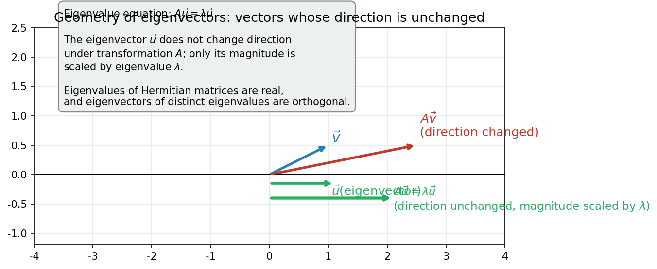
Fig. B.1: Geometric meaning of eigenvectors under a linear transformation. Under a linear transformation \(\hat{A}\), a general vector \(|v\rangle\) has both its direction and magnitude changed. However, an eigenvector \(|a\rangle\) preserves its direction, with only its magnitude changing by the eigenvalue factor \(a\).
🔵 Kai: Looking at Fig. B.1 "Geometric meaning of eigenvectors under a linear transformation", a general vector has both its direction and magnitude changed, but only the eigenvector keeps its direction and just stretches or shrinks. But if the eigenvalue \(a\) is negative, the direction reverses, right? Can we still say "the direction doesn't change"?
🟡 Lina: Sharp observation. Strictly speaking, if the eigenvalue is negative, the direction reverses—but we say "the direction doesn't change" in the sense that "it stays on the same line." A general vector gets thrown to a completely different direction, but an eigenvector stays on the original line. This property of "staying on the same line" is what's essential.
🟡 Lina: That's right. Applying \(\hat{A}\) just multiplies by \(a\). In quantum mechanics, eigenvalues correspond to "values obtained in measurements" and eigenvectors to "the state after measurement" (we'll cover this in detail in Ch. 12).
Finding Eigenvalues—The Characteristic Equation
🟡 Lina: The eigenvalue equation (B.36) can be rewritten as
This is a system of simultaneous linear equations with \(|a\rangle\) as the unknown, where the right-hand side is all zeros—this is called a homogeneous system of linear equations. \(|a\rangle = \mathbf{0}\) (all components zero) is always a solution, but the physically meaningful case is \(|a\rangle \neq \mathbf{0}\).
🔵 Kai: Is there a condition for a nonzero solution to exist?
🟡 Lina: Good question. There's an important theorem: a homogeneous system has a nonzero solution if and only if the determinant of the coefficient matrix is zero. Let me explain step by step. First, let me introduce the concept of an inverse matrix. In the world of numbers, there's a "partner" such that \(3 \times \frac{1}{3} = 1\), right? We call \(\frac{1}{3}\) the reciprocal of \(3\). The same applies to matrices: when a matrix \(M^{-1}\) exists satisfying \(M^{-1}M = MM^{-1} = \hat{1}\), we call \(M^{-1}\) the inverse matrix of \(M\). Here \(\hat{1}\) is the identity operator—the same one from the completeness relation in B.3—which in matrix representation is also written as the identity matrix \(I_N\). For \(2 \times 2\) it's \(\begin{pmatrix} 1 & 0 \\ 0 & 1 \end{pmatrix}\); for general \(N \times N\), it's the matrix with all diagonal entries equal to 1 and all others 0. It's the matrix that doesn't change any vector it acts on—that is, \(I_N \begin{pmatrix} v_1 \\ \vdots \\ v_N \end{pmatrix} = \begin{pmatrix} v_1 \\ \vdots \\ v_N \end{pmatrix}\).
🔵 Kai: So the inverse matrix is like "division for matrices"?
🟡 Lina: Yes, that's a good way to think about it. If the inverse matrix exists, then from \(M|a\rangle = \mathbf{0}\), multiplying both sides on the left by \(M^{-1}\) gives \(|a\rangle = M^{-1}\mathbf{0} = \mathbf{0}\)—only the trivial solution (why is \(M^{-1}\mathbf{0} = \mathbf{0}\)? Because in the definition of matrix multiplication \((AB)_{jk} = \sum_l A_{jl}B_{lk}\), all components of the zero vector are 0, so the dot product with any row is 0). In other words, if the inverse matrix exists, "only the trivial solution exists."
🔵 Kai: So for a nonzero eigenvector to exist, the inverse matrix must not exist.
🟡 Lina: Exactly. And the tool for determining whether "the inverse matrix doesn't exist" is the determinant. Let me explain what the determinant is. For a \(2 \times 2\) matrix \(M = \begin{pmatrix} a & b \\ c & d \end{pmatrix}\), the determinant is defined as
Geometrically, it equals the signed area of the parallelogram spanned by the two column vectors \(\begin{pmatrix} a \\ c \end{pmatrix}\) and \(\begin{pmatrix} b \\ d \end{pmatrix}\) of \(M\).
🔵 Kai: Does zero area mean the two vectors are pointing in the same direction?
🟡 Lina: Exactly. The two column vectors are parallel—one is a scalar multiple of the other. In this case, the matrix \(M\) crushes all vectors in the 2D plane onto a single line. Once crushed, you can't recover "where the original was," so the inverse matrix doesn't exist. And the direction that gets crushed—the direction that becomes zero when \(M\) is applied—exists, which is why \(M|a\rangle = \mathbf{0}\) allows a nonzero solution \(|a\rangle\).
⚪ Mei: "Zero area ⇔ crushing ⇔ no inverse"—everything connects through the geometric picture.
🟡 Lina: To summarize: determinant is zero ⇔ inverse matrix doesn't exist ⇔ nonzero solutions are allowed. Therefore, the condition for the eigenvalue equation \((\hat{A} - a\hat{1})|a\rangle = 0\) to have a nonzero solution is
In high school geometry, this corresponds to "the signed area of the parallelogram spanned by the two column vectors \(\begin{pmatrix} p \\ r \end{pmatrix}\) and \(\begin{pmatrix} q \\ s \end{pmatrix}\) of a matrix." Area zero = the two vectors are parallel = the matrix is degenerate.
For \(3 \times 3\), it's a bit longer, but let me explain the method of expanding along the first row. Just as the \(2 \times 2\) determinant corresponds to "the area of the parallelogram spanned by two column vectors," the \(3 \times 3\) determinant corresponds to "the volume of the parallelepiped spanned by three column vectors." If the volume is zero, the three vectors lie in the same plane—the matrix crushes 3D space into 2D—so by the same logic as the \(2 \times 2\) case, the inverse matrix doesn't exist. For the computation method: for each entry \(a, b, c\) in the first row, compute "the determinant of the \(2 \times 2\) submatrix obtained by removing the row and column that entry belongs to," and add them with alternating signs \(+, -, +\). Specifically:
- Contribution of \(a\): Remove \(a\)'s row (row 1) and column (column 1), leaving \(\begin{pmatrix} e & f \\ h & i \end{pmatrix}\) → \(+a(ei - fh)\)
- Contribution of \(b\): Remove \(b\)'s row (row 1) and column (column 2), leaving \(\begin{pmatrix} d & f \\ g & i \end{pmatrix}\) → \(-b(di - fg)\)
- Contribution of \(c\): Remove \(c\)'s row (row 1) and column (column 3), leaving \(\begin{pmatrix} d & e \\ g & h \end{pmatrix}\) → \(+c(dh - eg)\)
Putting it all together:
The signs alternate as \(+, -, +\) because the sign for the \((j,k)\) entry is determined by \((-1)^{j+k}\) (for row 1: \((-1)^{1+1} = +\), \((-1)^{1+2} = -\), \((-1)^{1+3} = +\)). This procedure is called cofactor expansion (it also appeared in Appendix A of General Relativity). For the scope of this book, being able to compute \(2 \times 2\) and \(3 \times 3\) determinants is sufficient.
🟡 Lina: We call (B.38) the characteristic equation.
🔵 Kai: Um, the reason the determinant must be zero is… if the determinant is nonzero, the inverse matrix exists, so \(|a\rangle = (\hat{A} - a\hat{1})^{-1} \mathbf{0} = \mathbf{0}\) is the only possibility, right? But can you always find values of \(a\) that make the determinant zero?
🟡 Lina: The first part is correct. If the inverse matrix exists, the solution is forced to be \(\mathbf{0}\). So for "a nonzero eigenvector to exist," the inverse must not exist—the determinant must be zero. The second question is also a good one. For an \(N \times N\) matrix, \(\det(\hat{A} - a\hat{1}) = 0\) is a degree-\(N\) polynomial equation in \(a\), so in the complex number domain, it always has \(N\) solutions (eigenvalues). This is a consequence of a mathematical theorem called the fundamental theorem of algebra—in high school you learned that "a quadratic equation always has two solutions in the complex number domain even when the discriminant is negative," right? This is the generalization to degree \(N\). The proof is advanced, but using just the conclusion is sufficient. So remember: "an \(N \times N\) matrix always has exactly \(N\) eigenvalues, counting multiplicity."
Concrete Example: Pauli Matrix \(\sigma_z\)
🟡 Lina: Let's practice with a 2-dimensional example. One of the Pauli matrices that appears in Ch. 5 and Ch. 17:
Find its eigenvalues and eigenvectors.
🔵 Kai: The characteristic equation is
So \(a = +1\) and \(a = -1\).
🔵 Kai: For \(a = +1\), solving \((\hat{\sigma}_z - \hat{1})|a\rangle = 0\):
So \(\eta = 0\). Normalizing gives \(|+\rangle = \begin{pmatrix} 1 \\ 0 \end{pmatrix}\). Doing the same for \(a = -1\)… \(\begin{pmatrix} 2 & 0 \\ 0 & 0 \end{pmatrix}\begin{pmatrix} \xi \\ \eta \end{pmatrix} = \begin{pmatrix} 0 \\ 0 \end{pmatrix}\), so \(\xi = 0\) and \(|-\rangle = \begin{pmatrix} 0 \\ 1 \end{pmatrix}\).
🔵 Kai: Ah, computing the inner product of the two eigenvectors: \(\langle +|-\rangle = 1 \cdot 0 + 0 \cdot 1 = 0\)—they're orthogonal. Do eigenvectors with different eigenvalues always have to be orthogonal?
🟡 Lina: Good observation. In fact, for Hermitian matrices, orthogonality can be proven. I'll prove it in the next section. And these \(|+\rangle\) and \(|-\rangle\) correspond to the "spin-up" and "spin-down" states of spin-1/2.
🔵 Kai: For non-Hermitian matrices, they might not be orthogonal?
🟡 Lina: That's right. For non-Hermitian matrices, eigenvalues can be complex, and there's no guarantee that eigenvectors are orthogonal. That's exactly why the condition of "being Hermitian" is physically important. Let's look at this in detail in the next section.
✅ Comprehension Check: How many eigenvalues does an \(N \times N\) matrix have at most?
Answer
\(N\), counting multiplicity. Because the characteristic equation is a degree-\(N\) polynomial in \(a\).
B.6 Hermitian Matrices—Why Measurement Values Are Real
🟡 Lina: The most important class of matrices in quantum mechanics is Hermitian matrices.
🟡 Lina: An operator \(\hat{A}\) is Hermitian (or self-adjoint) if
That is, taking the Hermitian conjugate returns the operator to itself. In terms of matrix elements:
Diagonal entries are real, and off-diagonal entries are complex conjugates of each other.
🔵 Kai: Why are Hermitian matrices important in quantum mechanics?
🟡 Lina: There are two decisive reasons.
Theorem 1: Eigenvalues of Hermitian Operators Are Real
🟡 Lina: Let's prove this. Given \(\hat{A}|a\rangle = a|a\rangle\), apply \(\langle a|\) from the left to both sides:
On the other hand, using the definition of the Hermitian conjugate (B.30) with \(|\psi\rangle = |\phi\rangle = |a\rangle\) (setting \(|\psi\rangle = |\phi\rangle = |a\rangle\) in both the left side \(\langle\phi|\hat{A}^\dagger|\psi\rangle\) and right side \(\langle\psi|\hat{A}|\phi\rangle^*\) of (B.30)):
Using Hermiticity \(\hat{A}^\dagger = \hat{A}\) on the left side:
Therefore \(\langle a|\hat{A}|a\rangle\) is real (it equals its own complex conjugate). From (B.42), \(\langle a|\hat{A}|a\rangle = a\langle a|a\rangle\); the left side is real and \(\langle a|a\rangle > 0\) is also real, so \(a\) must be real. \(\square\)
🔵 Kai: Wow, just using Hermiticity is enough to show the eigenvalues are real.
🟡 Lina: In other words, since measurement values must be real, operators representing observables must be Hermitian—this is the physical reason for requiring Hermiticity.
⚪ Mei: I see: "eigenvalues = measurement values," and Hermiticity guarantees the eigenvalues are real.
Theorem 2: Eigenvectors Belonging to Different Eigenvalues Are Orthogonal
🟡 Lina: Let \(\hat{A}|a\rangle = a|a\rangle\) and \(\hat{A}|a'\rangle = a'|a'\rangle\) with \(a \neq a'\).
On the other hand, let's take the Hermitian conjugate of both sides of \(\hat{A}|a'\rangle = a'|a'\rangle\). "Taking the Hermitian conjugate of an equation" means rewriting both sides into a form that can be "placed on the left side of an inner product"—that is, into bra form (also called "converting a ket equation to a bra equation"). Let me state the rule first: in general, the Hermitian conjugate of the equation \(\hat{X}|\alpha\rangle = c|\beta\rangle\) is \(\langle\alpha|\hat{X}^\dagger = c^*\langle\beta|\). What's happening is: the ket \(|\alpha\rangle\) becomes the bra \(\langle\alpha|\), the operator \(\hat{X}\) gets a dagger \(\dagger\), and the scalar \(c\) becomes the complex conjugate \(c^*\)—this is a combination of (B.33) and (B.35). Intuitively, you can think of it as the operator version of "swapping left and right in an inner product introduces a complex conjugate" (B.7).
🔵 Kai: Wait a moment. "Converting a ket equation to a bra equation"—what operation is that concretely? Is it like transposing both sides and taking the complex conjugate?
🟡 Lina: Good question. In matrix representation, that's exactly it—rewriting a column vector equation as a row vector equation means transposing and taking the complex conjugate. But in the abstract operator language, it can be verified as follows. Consider the inner product with an arbitrary vector \(|\gamma\rangle\): from \(\hat{X}|\alpha\rangle = c|\beta\rangle\), apply \(\langle\gamma|\) from the left to get \(\langle\gamma|\hat{X}|\alpha\rangle = c\langle\gamma|\beta\rangle\). By the definition of Hermitian conjugate (B.30), \(\langle\gamma|\hat{X}|\alpha\rangle = \langle\alpha|\hat{X}^\dagger|\gamma\rangle^*\), so taking the complex conjugate gives \(\langle\alpha|\hat{X}^\dagger|\gamma\rangle = c^*\langle\beta|\gamma\rangle\). Since this holds for arbitrary \(|\gamma\rangle\), we get \(\langle\alpha|\hat{X}^\dagger = c^*\langle\beta|\).
Applying this to \(\hat{A}|a'\rangle = a'|a'\rangle\) gives \(\langle a'|\hat{A}^\dagger = a'^*\langle a'|\). Using Hermiticity \(\hat{A}^\dagger = \hat{A}\) and Theorem 1 (\(a'\) is real so \(a'^* = a'\)):
Acting on \(|a\rangle\) from the right:
Subtracting (B.44) from (B.45):
Since \(a \neq a'\), we have \(\langle a'|a\rangle = 0\). \(\square\)
🔵 Kai: Different eigenvalues automatically mean orthogonal! But what if there are multiple vectors with the same eigenvalue? Are they orthogonal too?
🟡 Lina: Good question. Multiple eigenvectors with the same eigenvalue—called degeneracy—are not automatically orthogonal. But the Gram–Schmidt orthogonalization procedure can be used to orthogonalize them, so ultimately one can always construct an orthonormal basis from the eigenvectors of a Hermitian operator.
✅ Comprehension Check: In the proof that eigenvectors of a Hermitian operator belonging to different eigenvalues are orthogonal, what is the key step?
Answer
Compute \(\langle a'|\hat{A}|a\rangle\) in two ways (acting to the right gives \(a\langle a'|a\rangle\), acting to the left gives \(a'\langle a'|a\rangle\)), and taking the difference gives \((a - a')\langle a'|a\rangle = 0\). Since \(a \neq a'\), it follows that \(\langle a'|a\rangle = 0\) (orthogonality).
Theorem 3 (Diagonalization): Hermitian Matrices Can Be Diagonalized by Unitary Transformations
🟡 Lina: If we choose the orthonormal eigenvectors \(\{|a_1\rangle, |a_2\rangle, \ldots, |a_N\rangle\}\) of a Hermitian matrix \(\hat{A}\) as our basis, the matrix representation of \(\hat{A}\) becomes
The eigenvalues line up along the diagonal. This is called diagonalization.
🟡 Lina: In quantum mechanics, this theorem is often written in the form of a spectral decomposition:
This is the form of the completeness relation (B.21) with eigenvalues \(a_k\) attached as "weights" in front of \(|e_k\rangle\langle e_k|\).
⚪ Mei: So we've decomposed the operator into a sum of "eigenvalue × projection operator."
🟡 Lina: Exactly. This forms the mathematical foundation of measurement in quantum mechanics.
✅ Comprehension Check: What is the spectral decomposition of a Hermitian operator?
Answer
Writing a Hermitian operator \(\hat{A}\) as \(\hat{A} = \sum_k a_k |a_k\rangle\langle a_k|\). It's the representation as a sum of eigenvalues \(a_k\) and their corresponding projection operators \(|a_k\rangle\langle a_k|\), and forms the mathematical foundation of measurement theory in quantum mechanics.
Concrete Example: The Pauli Matrices Are All Hermitian
🟡 Lina: Let's verify this.
🔵 Kai: \(\hat{\sigma}_x\) is the same when transposed and has real entries, so \(\hat{\sigma}_x^\dagger = \hat{\sigma}_x\). For \(\hat{\sigma}_y\), transposing makes the \((1,2)\) entry \(i\) and the \((2,1)\) entry \(-i\), but then taking the complex conjugate returns it to the original. \(\hat{\sigma}_z\) is diagonal with real entries, so it's obvious. They're all Hermitian.
🟡 Lina: Perfect. The eigenvalues are all \(\pm 1\), which are real. This corresponds to the fact that the eigenvalues \(\pm\hbar/2\) of the spin angular momentum \(S_i = (\hbar/2)\sigma_i\) are real.
✅ Comprehension Check: What is the definition equation of Hermiticity used when proving that eigenvalues of a Hermitian operator are real?
Answer
\(\hat{A}^\dagger = \hat{A}\). This allows the left side of \(\langle a|\hat{A}|a\rangle = a\langle a|a\rangle\) to also be written as \(a^*\langle a|a\rangle\), from which \(a = a^*\) (real) is derived.
B.7 Unitary Matrices—Transformations That Preserve Probability
🟡 Lina: The next important class is unitary matrices.
That is, \(\hat{U}^\dagger = \hat{U}^{-1}\) (the inverse matrix equals the Hermitian conjugate).
🔵 Kai: Hermitian matrices have \(\hat{A}^\dagger = \hat{A}\), and unitary matrices have \(\hat{U}^\dagger = \hat{U}^{-1}\). Similar but different.
🟡 Lina: Good comparison. Hermitian means "equals itself," unitary means "equals its inverse." Their physical roles are different too. Hermitian operators represent observables, while unitary operators represent transformations of states (time evolution and basis changes).
Important Properties of Unitary Transformations
🟡 Lina: The reason unitary transformations are physically important is that they preserve inner products.
With \(|\psi'\rangle = \hat{U}|\psi\rangle\) and \(|\phi'\rangle = \hat{U}|\phi\rangle\):
⚪ Mei: If the inner product doesn't change, then the norm is also preserved. \(\langle\psi'|\psi'\rangle = \langle\psi|\psi\rangle\).
🟡 Lina: Exactly. So the normalization condition \(\langle\psi|\psi\rangle = 1\) is maintained after the transformation.
🔵 Kai: I understand that normalization is preserved, but what does that mean physically?
🟡 Lina: Good question. In quantum mechanics, \(|\langle\phi|\psi\rangle|^2\) is related to probability (we'll cover details in Ch. 5). The fact that the inner product is preserved means that unitary transformations are probability-preserving transformations.
Unitary Matrices as Basis Changes
🟡 Lina: The transformation from one orthonormal basis \(\{|e_k\rangle\}\) to another orthonormal basis \(\{|e'_k\rangle\}\) is given by a unitary matrix \(\hat{U}\):
Taking the Hermitian conjugate of (B.52):
The matrix elements of an operator \(\hat{A}\) in the new basis are then:
Here I substituted (B.53) and (B.52). In matrix language, this is a similarity transformation:
Here \(\hat{A}'\) denotes the matrix representation of operator \(\hat{A}\) in the new basis \(\{|e'_k\rangle\}\).
🔵 Kai: To view an operator in a different basis, you sandwich it between unitary matrices on both sides.
🟡 Lina: There are quantities that don't change under similarity transformations: the trace (sum of diagonal elements), the determinant, and the eigenvalues.
🔵 Kai: It's reassuring that eigenvalues don't depend on the basis. It would be a problem if measurement results changed depending on your choice of coordinate system.
🟡 Lina: Exactly. The results of physical measurements don't depend on the observer's "choice of basis"—that's the physical meaning of unitary transformations.
✅ Comprehension Check: Name three quantities of a matrix that are invariant under unitary (similarity) transformations.
Answer
Trace (sum of diagonal elements), determinant, and eigenvalues. These are invariants independent of the choice of basis, guaranteeing that physical measurement results don't depend on the observer's basis selection.
Concrete Example: Transformation from the \(S_z\) Basis to the \(S_x\) Basis
🟡 Lina: Let me preview an example from spin in Ch. 5. From the \(S_z\) eigenvectors \(|+\rangle = \begin{pmatrix} 1 \\ 0 \end{pmatrix}\), \(|-\rangle = \begin{pmatrix} 0 \\ 1 \end{pmatrix}\) to the \(S_x\) eigenvectors
the transformation matrix is
🔵 Kai: Let me check. All entries are real, so taking the complex conjugate doesn't change anything. And swapping rows and columns gives the same form, so… \(\hat{U}^\dagger = \hat{U}\)?
🟡 Lina: Yes. This matrix has real entries and is symmetric (unchanged under transposition), so \(\hat{U}^\dagger = \hat{U}\). Therefore the unitarity condition \(\hat{U}^\dagger \hat{U} = \hat{1}\) becomes equivalent to \(\hat{U}^2 = \hat{1}\). Computing explicitly: \(\frac{1}{2}\begin{pmatrix} 1 & 1 \\ 1 & -1 \end{pmatrix}\begin{pmatrix} 1 & 1 \\ 1 & -1 \end{pmatrix} = \frac{1}{2}\begin{pmatrix} 2 & 0 \\ 0 & 2 \end{pmatrix} = \hat{1}\). Indeed unitary.
⚪ Mei: Squaring gives the identity matrix back, so applying the transformation twice returns you to the original.
🟡 Lina: By the way, this matrix happens to be a special case that is both Hermitian and unitary. General unitary matrices usually have \(\hat{U}^\dagger \neq \hat{U}\), so don't think "unitary = Hermitian." And being both Hermitian and unitary means that applying it twice returns you to the original.
🔵 Kai: \(\hat{U}|+\rangle = \frac{1}{\sqrt{2}}\begin{pmatrix} 1 \\ 1 \end{pmatrix} = |+\rangle_x\) checks out too. But why does "arranging the new basis as column vectors" give the transformation matrix?
🟡 Lina: Good question. Recall the matrix-vector product. When you multiply the matrix \(\hat{U}\) by \(|e_1\rangle = \begin{pmatrix} 1 \\ 0 \end{pmatrix}\), the result is just the first column of \(\hat{U}\), right? Similarly, multiplying by \(|e_2\rangle = \begin{pmatrix} 0 \\ 1 \end{pmatrix}\) gives the second column. So the definition \(\hat{U}|e_k\rangle = |e'_k\rangle\) from (B.52) means "the \(k\)-th column of \(\hat{U}\) = the components of the \(k\)-th new basis vector \(|e'_k\rangle\)." That's why the new basis vectors appear as columns.
🔵 Kai: Ah, I see. Multiplying by \(\begin{pmatrix} 1 \\ 0 \end{pmatrix}\) "selects" only the first column, so the destination basis is stored in the columns.
✅ Comprehension Check: What does it mean for a unitary transformation to "preserve probability"?
Answer
A unitary transformation preserves inner products (\(\langle\phi'|\psi'\rangle = \langle\phi|\psi\rangle\)). In quantum mechanics, \(|\langle\phi|\psi\rangle|^2\) corresponds to transition probability, so probability doesn't change before and after a unitary transformation.
📝 Exercises:
- Compute \(\hat{U}^\dagger \hat{\sigma}_x \hat{U}\) using \(\hat{U}\) from equation (B.57) and confirm the result is the diagonal matrix \(\begin{pmatrix} 1 & 0 \\ 0 & -1 \end{pmatrix}\) (Hint: This \(\hat{U}\) satisfies \(\hat{U} = \hat{U}^\dagger = \hat{U}^{-1}\). Since the column vectors of \(\hat{U}\) are eigenvectors of \(\hat{\sigma}_x\), \(\hat{U}^\dagger \hat{\sigma}_x \hat{U}\) gives \(\hat{\sigma}_x\) expressed in the eigenbasis—that is, a matrix with eigenvalues \(+1, -1\) on the diagonal) → Problem A-1. Basis Transformation by Unitary Matrices and Transformation Rules for Matrix Representations
B.8 Tensor Product—Combining Two Systems
🟡 Lina: In quantum mechanics, we often deal with "composite systems" formed by combining two independent systems. For example, the spins of two electrons, or a particle's position and spin. The tool for this is the tensor product.
🔵 Kai: What's a tensor product?
🟡 Lina: Intuitively, it's the operation of pairing "the state of system 1" with "the state of system 2" to form a single state. For example, if you simultaneously consider the heads/tails of a coin (2 possibilities) and the face of a die (6 possibilities), the combinations are \(2 \times 6 = 12\), right? The tensor product formalizes this "combination" in the language of vector spaces.
⚪ Mei: The number of combinations is multiplicative.
🟡 Lina: Mathematically, let the vector space where system 1's states live (with inner product—we call this a Hilbert space, which I'll formally define in B.9; for now think of it as "a vector space with an inner product defined") be \(\mathcal{H}_1\) (dimension \(N_1\)). \(\mathcal{H}\) is the standard symbol for Hilbert space. Similarly, let system 2's space be \(\mathcal{H}_2\) (dimension \(N_2\)). The Hilbert space of the composite system is
and the dimension is \(N_1 \times N_2\). The symbol \(\otimes\) denotes the "tensor product."
🟡 Lina: When system 1 is in state \(|\psi\rangle \in \mathcal{H}_1\) and system 2 is in state \(|\phi\rangle \in \mathcal{H}_2\), the composite system's state is written as
This is also abbreviated as \(|\psi\rangle|\phi\rangle\) or \(|\psi, \phi\rangle\).
Computation Rules for Tensor Products
🟡 Lina: The tensor product follows these rules.
(1) Linearity:
(2) Inner product:
Compute the inner product of each system separately and multiply them.
Tensor Product of Matrices (Kronecker Product)
🟡 Lina: In matrix representation, the tensor product is expressed as the Kronecker product. The Kronecker product of an \(m \times n\) matrix \(A\) and a \(p \times q\) matrix \(B\) is an \(mp \times nq\) matrix:
🟡 Lina: Let's look at a concrete example. With \(\mathcal{H}_1 = \mathcal{H}_2 = \mathbb{C}^2\):
🔵 Kai: 2-dimensional × 2-dimensional = 4-dimensional.
⚪ Mei: Combining two spin-1/2 systems gives a 4-dimensional space.
Entangled States
🟡 Lina: Within the tensor product space, there exist vectors that cannot be written in the form \(|\psi\rangle \otimes |\phi\rangle\). For example:
🔵 Kai: Can't this be decomposed into the form \(|\psi\rangle \otimes |\phi\rangle\)?
🟡 Lina: It can't. Let's prove this by contradiction. Suppose \(|\Psi\rangle = (a|+\rangle + b|-\rangle) \otimes (c|+\rangle + d|-\rangle)\) could be written this way. Expanding:
Compare the coefficients with (B.65).
🔵 Kai: Let's see, the coefficient of \(|+\rangle|+\rangle\) is zero in (B.65), so \(ac = 0\). The coefficient of \(|+\rangle|-\rangle\) is \(1/\sqrt{2}\), so \(ad = 1/\sqrt{2}\). For \(|-\rangle|+\rangle\) it's \(-1/\sqrt{2}\), so \(bc = -1/\sqrt{2}\). And \(|-\rangle|-\rangle\) is zero, so \(bd = 0\).
🔵 Kai: Since \(ac = 0\), either \(a = 0\) or \(c = 0\). But if \(a = 0\), then \(ad = 0\) which contradicts \(1/\sqrt{2}\)… If \(c = 0\), then \(bc = 0\) which contradicts \(-1/\sqrt{2}\)… Wait, either way leads to a contradiction?
🟡 Lina: Exactly. Either case leads to a contradiction, so it cannot be written in tensor product form—it's an entangled state. "You cannot assign an independent state to each subsystem"—that's the essence of entanglement.
⚪ Mei: A proof by contradiction showing that "assuming it can be decomposed necessarily leads to a contradiction."
🟡 Lina: States that cannot be decomposed into tensor product form like this are called entangled states. We'll cover them in detail in Chapters 23–24, but they represent one of the most surprising features of quantum mechanics.
✅ Comprehension Check: What is an entangled state?
Answer
A state vector of a composite system that cannot be decomposed into a tensor product \(|\psi\rangle \otimes |\phi\rangle\) of state vectors of the individual subsystems. For example, \(\frac{1}{\sqrt{2}}(|+\rangle \otimes |-\rangle - |-\rangle \otimes |+\rangle)\) is an entangled state.
✅ Comprehension Check: What is the dimension of the tensor product space of two 2-dimensional Hilbert spaces?
Answer
\(2 \times 2 = 4\) dimensions.
📝 Exercises:
- Show that \(|\Psi\rangle = \frac{1}{\sqrt{2}}(|+\rangle \otimes |+\rangle + |-\rangle \otimes |-\rangle)\) is an entangled state → Problem A-2. Tensor Product Space and Construction of the Bell Basis
B.9 Extension to Infinite-Dimensional Hilbert Spaces—Functions Become Vectors Too
🟡 Lina: So far we've been working in finite-dimensional \(\mathbb{C}^N\), but from Ch. 7 onward, where we deal with wave functions, we'll need infinite-dimensional Hilbert spaces. Let me formally define it here: a Hilbert space is "a vector space with an inner product defined that is also complete."
🔵 Kai: What does "complete" mean?
🟡 Lina: Intuitively, it means "the destination of a sequence of points that get increasingly close actually lies within the space." For example, the sequence of rational numbers \(1, 1.4, 1.41, 1.414, \ldots\) approaches \(\sqrt{2}\), but \(\sqrt{2}\) is not a rational number, so the set of rational numbers is "not complete." The set of real numbers includes \(\sqrt{2}\), so it's complete. The same applies to vector spaces: "the limit of a sequence of vectors that keep getting closer actually belongs to the space" is what we call completeness. Finite-dimensional \(\mathbb{C}^N\) is automatically complete, so once we defined the inner product in B.2, it was already a Hilbert space. In infinite dimensions, "whether it's complete" becomes nontrivial, but \(L^2\) has been proven to be complete, so it's a Hilbert space.
⚪ Mei: In finite dimensions completeness is automatic, but in infinite dimensions it requires proof—that's the subtle point.
🟡 Lina: Finally, let me organize "what changes" when transitioning from finite to infinite dimensions.
The Function Space \(L^2\) Is a Hilbert Space
🟡 Lina: Let me re-formulate the space of square-integrable functions \(L^2\) from B.1 as a Hilbert space.
The inner product of two functions \(f(x)\) and \(g(x)\) is defined as
This satisfies all three properties (B.6)–(B.8).
🔵 Kai: The finite-dimensional \(\sum_k z_k^* z'_k\) is just replaced by \(\int f^* g\, dx\).
🟡 Lina: That intuition is correct. The sum \(\sum\) corresponds to the integral \(\int\), and the component \(z_k\) corresponds to the function value \(f(x)\). However, this "replacement" introduces several subtle issues.
Correspondence Table Between Finite and Infinite Dimensions
🟡 Lina: Let me summarize the correspondence in a table.
Table B.2: Correspondence between finite and infinite dimensions
| Finite-dimensional \(\mathbb{C}^N\) | Infinite-dimensional \(L^2\) |
|---|---|
| Vector \(\lvert\psi\rangle = \sum_k c_k \lvert e_k\rangle\) | Function \(f(x) = \sum_n c_n f_n(x)\) or \(\int c(k) f_k(x)\, dk\) |
| Component \(c_k = \langle e_k\lvert\psi\rangle\) | Expansion coefficient \(c_n = \langle f_n\lvert f\rangle = \int f_n^* f\, dx\) |
| Inner product \(\sum_k z_k^* z'_k\) | Inner product \(\int f^* g\, dx\) |
| Kronecker delta \(\delta_{jk}\) | Dirac delta function \(\delta(x - x')\) |
| Completeness \(\sum_k \lvert e_k\rangle\langle e_k\rvert = \hat{1}\) | Completeness \(\sum_n \lvert f_n\rangle\langle f_n\rvert = \hat{1}\) or \(\int \lvert x\rangle\langle x\rvert\, dx = \hat{1}\) |
| Matrix \(A_{jk}\) | Integral kernel \(A(x, x')\) |
Subtlety 1: Discrete and Continuous Spectra
🟡 Lina: In finite dimensions, eigenvalues are always discrete (isolated values), but in infinite dimensions, a continuous spectrum can appear.
🔵 Kai: What's a continuous spectrum?
🟡 Lina: For example, the eigenvalues of the momentum operator \(\hat{p} = -i\hbar\, d/dx\) for a free particle take any real value \(p\). They're not isolated but continuous. Writing out the eigenvalue equation \(\hat{p}\,f_p(x) = p\,f_p(x)\) gives \(-i\hbar\, df_p/dx = p\,f_p\), that is, \(df_p/dx = (ip/\hbar)\,f_p\). This is the question "what function, when differentiated, gives a constant multiple of itself?" In high school you learned that differentiating \(e^x\) gives \(e^x\) itself. In general, differentiating \(e^{\alpha x}\) gives \(\alpha e^{\alpha x}\)—a factor of \(\alpha\) times itself. And it can be proven that "the only function whose derivative is a constant multiple of itself" is the exponential function. So the solution to \(df_p/dx = (ip/\hbar)f_p\) must be \(f_p(x) \propto e^{ipx/\hbar}\).
🔵 Kai: Wait, so the eigenfunction is \(e^{ipx/\hbar}\) and \(p\) can be any real number? That's an infinitely extending wave, right?
🟡 Lina: Yes. The normalization constant must be chosen so that the delta function normalization (B.68) holds. The result is
This function cannot be normalized in the ordinary sense (\(\int |f_p|^2\, dx = \infty\)). Instead, we use delta function normalization with the Dirac delta function \(\delta(p - p')\). The delta function is, intuitively, "a special function that has an infinitely sharp peak only at \(x = 0\) and is zero elsewhere," satisfying \(\int_{-\infty}^{\infty} \delta(x)\, dx = 1\)—think of it as the continuous version of the Kronecker delta \(\delta_{jk}\). As an image, consider a rectangle of width \(\epsilon\) and height \(1/\epsilon\). The area is always 1, but as \(\epsilon \to 0\), the width collapses to zero and the height stretches to infinity—that limit is the delta function. \(\delta(p - p')\) is the version that "peaks only at \(p = p'\)."
The essential point is that the delta function is used "multiplied by another function inside an integral": \(\int f(x)\,\delta(x - a)\,dx = f(a)\)—that is, "the delta function picks out the value of the function at \(x = a\) from within the integral." This is the continuous version of the Kronecker delta \(\sum_k f_k\,\delta_{jk} = f_j\). The rigorous definition is covered in Appendix C, but for now understand it by analogy with the discrete case: "\(p = p'\) corresponds to 1, \(p \neq p'\) corresponds to 0." Delta function normalization is the condition written as
This is the continuous version corresponding to \(\langle e_j|e_k\rangle = \delta_{jk}\) for discrete bases. Although it's called "normalization," the fact that \(\delta(0) = \infty\) when \(p = p'\) may seem strange—but this is not normalization in the sense of "norm equals 1." Rather, it expresses that "eigenfunctions of different eigenvalues are orthogonal" and "the overlap between eigenfunctions of the same eigenvalue is consistently regulated by a certain convention." Just as \(\delta_{jk}\) in the discrete case meant "1 if \(j = k\), 0 if \(j \neq k\)," in the continuous case \(\delta(p - p')\) plays the same role. And the normalization constant \(1/\sqrt{2\pi\hbar}\) is the value chosen so that exactly this (B.68) holds. Why this particular value emerges will become naturally clear when you learn Fourier transforms in Appendix C.
🔵 Kai: Hmm, being told "with this constant, (B.68) holds" doesn't quite satisfy me unless I actually see the computation of \(\int f_{p'}^* f_p\, dx\) giving \(\delta(p - p')\)…
🟡 Lina: I completely understand that feeling. The actual computation requires Fourier transform formulas, which we'll develop in Appendix C. There we'll derive the identity "multiplying plane waves of different momenta and integrating over all space gives a delta function," and using that, you can verify (B.68). For now, think of it as "verification is deferred to Appendix C."
🔵 Kai: Got it. If it can be confirmed by calculation, I'm satisfied.
⚪ Mei: For discrete spectra it's the Kronecker delta \(\delta_{jk}\), for continuous spectra it's the Dirac delta \(\delta(p - p')\). The same pattern as sums \(\sum\) being replaced by integrals \(\int\).
Subtlety 2: Completeness of Eigenfunction Systems
🟡 Lina: In finite dimensions, it can be proven as a theorem that eigenvectors of a Hermitian matrix form a complete set. But in infinite dimensions, this generally cannot be proven.
🔵 Kai: Why can't it be proven in infinite dimensions?
🟡 Lina: Intuitively, in finite dimensions the characteristic equation becomes a degree-\(N\) polynomial in \(a\), right? In the complex number domain, a degree-\(N\) polynomial always has \(N\) roots—this is a mathematical theorem called the "fundamental theorem of algebra." Think of it as the generalization to degree \(N\) of the high school fact that "a quadratic equation always has two solutions from the quadratic formula." For Hermitian matrices, it's further guaranteed that "the eigenvectors form an orthonormal complete set" (as we saw in Theorem 3 of B.6). So for finite-dimensional Hermitian matrices, completeness holds automatically.
🔵 Kai: I see, in finite dimensions "a degree-\(N\) equation has \(N\) solutions" ensures everything is found.
🟡 Lina: But in infinite dimensions, the very concept of "what degree polynomial" disappears, and there are issues with the domain of operators, so whether the eigenvectors span the entire space must be investigated individually for each operator. For "well-behaved" operators that appear in physics, it often holds, but it's not guaranteed as a general theorem.
🔵 Kai: So what do we do?
🟡 Lina: In quantum mechanics, we adopt as a postulate (axiom) that the eigenfunctions of Hermitian operators corresponding to observables form a complete set. This is not something to be proven mathematically, but an assumption accepted as the starting point of the physical model.
⚪ Mei: What could be proven as a theorem in finite dimensions must be postulated in infinite dimensions—that shows how much harder infinite dimensions are to handle.
✅ Comprehension Check: In infinite-dimensional Hilbert space, how is the completeness of eigenfunctions of Hermitian operators guaranteed?
Answer
Unlike the finite-dimensional case, it generally cannot be proven mathematically. In quantum mechanics, it is adopted as a postulate (axiom) that "eigenfunctions of Hermitian operators corresponding to observables form a complete set."
Subtlety 3: Domain of Operators
🟡 Lina: In infinite dimensions, an operator may not be able to "act on all vectors." For example, the differential operator \(\hat{p} = -i\hbar\, d/dx\) cannot act on functions that aren't differentiable. The set of vectors on which an operator can act is called its domain.
🔵 Kai: Didn't we have to worry about this in finite dimensions?
🟡 Lina: In finite dimensions, a matrix can act on every vector, so domain issues don't arise. But in infinite dimensions, when determining "whether an operator is Hermitian," the domain must be carefully specified. Strictly speaking, self-adjoint and Hermitian are different concepts in infinite dimensions, and the physically correct one is self-adjoint.
🔵 Kai: So which one does this book use?
🟡 Lina: Like many physics textbooks, in Quantum Mechanics we won't distinguish between "Hermitian" and "self-adjoint" as long as it doesn't cause problems in standard physics calculations. But keep in mind that such subtleties exist.
Summary: What You Learned in Finite Dimensions Also Works in Infinite Dimensions
🟡 Lina: What I want you to feel reassured about is that the concepts learned in finite dimensions—inner products, orthonormal bases, completeness relations, Hermitian operators, unitary operators—can essentially be used in the same form in infinite dimensions. The differences are:
- Sums \(\sum\) may be replaced by integrals \(\int\)
- For continuous spectra, delta function normalization is used
- Care must be taken with the domain of operators
If you keep these 3 points in mind, you'll be able to smoothly enter the wave function discussions from Ch. 7 onward.
🔵 Kai: If there are only 3 things to watch out for, I think I can manage.
✅ Comprehension Check: What are the biggest differences between finite-dimensional and infinite-dimensional Hilbert spaces? Name three.
Answer
(1) Not just discrete spectra but also continuous spectra can appear. (2) Eigenfunctions of continuous spectra cannot be normalized in the ordinary sense; delta function normalization using the Dirac delta function is used. (3) Care must be taken with the domain of operators, and the distinction between "Hermitian" and "self-adjoint" can arise.
Summary of This Appendix
🟡 Lina: Let me organize the content of this Appendix in terms of its correspondence with quantum mechanics.
Table B.3: Summary of mathematical concepts and their quantum mechanics correspondence
| Mathematical Concept | Role in Quantum Mechanics | Chapters Where It Appears |
|---|---|---|
| Complex vector space | Space where quantum states live | Ch. 4– |
| Inner product \(\langle\phi\lvert\psi\rangle\) | Probability amplitude | Ch. 4– |
| Orthonormal basis | Measurement basis | Ch. 5– |
| Completeness relation | State expansion, probabilities sum to 1 | Ch. 5– |
| Hermitian operator | Observables (position, momentum, energy, etc.) | Ch. 8, Ch. 11– |
| Eigenvalues/eigenvectors | Measurement values / post-measurement states | Ch. 5, Ch. 12 |
| Unitary operator | Time evolution, basis changes | Ch. 6, Ch. 13 |
| Tensor product | State space of composite systems | Ch. 18, Ch. 23–Ch. 24 |
🔵 Kai: Everything is connected.
🟡 Lina: Yes. Linear algebra is the "grammar" of quantum mechanics. Refer back to this Appendix as you read through the main text.
Preview of Next Chapter
🟡 Lina: In Appendix C, we'll cover Fourier analysis and the \(\delta\) function. In this Appendix I said "sums \(\sum\) get replaced by integrals \(\int\)"—the concrete mechanism for that is the Fourier transform. We'll develop the tools essential for eigenfunction expansions with continuous spectra and for bridging the momentum and position representations.
🔵 Kai: Will we learn the true nature of the delta function?
🟡 Lina: Yes. The delta function is "not an ordinary function," but it can be naturally understood in the language of Fourier transforms. Look forward to it.
Practice Problems
📝 Exercises:
- Norm and normalization of a vector in \(\mathbb{C}^2\) → Problem B-1. Norm Calculation of a Vector in \(\mathbb{C}^2\)
- Computing the Hermitian conjugate → Problem B-6. Calculating the Hermitian Conjugate
- Determining linear independence → Problem B-8. Determining Linear Independence
- Gram–Schmidt orthogonalization → Problem M-1. Gram–Schmidt Orthogonalization
- Diagonalization by unitary transformation → Problem A-1. Basis Transformation by Unitary Matrices and Transformation Rules for Matrix Representations
- Proof of an entangled state → Problem A-2. Tensor Product Space and Construction of the Bell Basis
References
- J. J. Sakurai, J. Napolitano, Modern Quantum Mechanics (3rd ed.), Cambridge University Press — The mathematical framework section of Ch.1. Referenced for Dirac notation, operators, eigenvalue problems, and basis change formulations.
- D. J. Griffiths, D. F. Schroeter, Introduction to Quantum Mechanics (3rd ed.), Cambridge University Press — Ch.3 (formalism): referenced for the definition of Hilbert space, proofs of Hermitian operator theorems, and treatment of continuous spectra.
- 清水明『新版 量子論の基礎——その本質のやさしい理解のために』サイエンス社 — Ch.3: referenced for the construction of complex Hilbert spaces, inner product axioms, Pauli matrix eigenvalue problems, and the concept of rays.
Feedback on this page
Let us know if something was unclear, incorrect, or could be improved.