Chapter 2: Review of Special Relativity and Lorentz Invariance
Story so far:
In Ch. 1, we confirmed that when trying to simultaneously satisfy quantum mechanics and special relativity, particle creation and annihilation become unavoidable, and that a new framework called "quantum field theory" is needed to describe this. We revisited the difficulties of the Klein-Gordon equation and Dirac equation foreshadowed in Quantum Mechanics Ch. 27, and built a bridge to the worldview that "particles are vibrational modes of fields."
Goals of this chapter
- Review the mathematical tools of special relativity (Lorentz transformations, Minkowski metric, 4-vectors, raising and lowering indices, Einstein summation convention) and newly acquire three perspectives particularly important for quantum field theory—(i) the sign convention \((+,-,-,-)\), (ii) classification of the Lorentz group and the Poincaré group, (iii) the practical skill of determining Lorentz covariance just by checking "index balance"
- This prepares the foundation for writing down Lagrangians and deriving field equations in subsequent chapters
2.1 A Quick Tour of the Mathematical Skeleton of Special Relativity
🟡 Lina: In Ch. 1, I mentioned that quantum field theory is "a theory that fuses quantum mechanics and special relativity." Today our goal is to organize the mathematical skeleton of special relativity into a form usable in quantum field theory.
🔵 Kai: We already covered special relativity and the mathematics of Minkowski spacetime in General Relativity Ch. 3 and General Relativity Ch. 4, didn't we? Won't this overlap?
🟡 Lina: Sharp question. The core physical content is the same, so in this chapter I'll take General Relativity Chapters 3–4 as prerequisites and quickly confirm only the results. Instead, I'll spend time on perspectives newly needed for quantum field theory—the classification of the Lorentz group, the Poincaré group, and the practical skill of determining covariance through "index balance."
⚪ Mei: So people who've already studied General Relativity Chapters 3–4 can just glance at the results in this section and move on.
🟡 Lina: Exactly. Let me summarize the key points in a table.
Mathematical skeleton of special relativity (summary of General Relativity Chapters 3–4)
Lorentz transformation (\(x\)-direction boost) — General Relativity Ch. 3
Using rapidity \(\varphi\) (\(\tanh\varphi = v\)), this can be written as a "hyperbolic rotation" in the same form as a rotation—see General Relativity Ch. 3.
4-vectors and indices — General Relativity Ch. 4
Greek indices \(\mu, \nu, \ldots\) run over \(0, 1, 2, 3\) (spacetime); Latin indices \(i, j, \ldots\) run over \(1, 2, 3\) (space only).
Einstein summation convention — When the same index appears once upstairs and once downstairs, sum from \(0\) to \(3\). The \(\sum\) is omitted.
Raising and lowering indices — Lower indices with the metric tensor \(\eta_{\mu\nu}\); raise them with the inverse metric \(\eta^{\mu\nu}\).
4-momentum and mass-shell condition — General Relativity Ch. 4
🔵 Kai: What about natural units \(c = \hbar = 1\)?
🟡 Lina: We introduced \(c = 1\) in General Relativity Ch. 4. In quantum field theory, since we're also fusing quantum mechanics, we additionally set \(\hbar = 1\)—this is called "natural units of particle physics." For the detailed conventions, refer to the "Related unit systems" note at the end of General Relativity General Relativity Ch. 4.
Adding \(\hbar = 1\) makes energy, mass, and frequency all have the same dimension. Why frequency too? Because \(E = \hbar\omega\) with \(\hbar = 1\) gives \(E = \omega\)—meaning frequency can be measured directly in units of energy. Similarly, \(E = mc^2\) with \(c = 1\) gives \(E = m\), so mass also has the same dimension as energy.
🔵 Kai: Mass and frequency both have the same dimension as energy... so you can write the electron mass in MeV?
🟡 Lina: Exactly. For example, the electron mass \(m_e \approx 0.511\,\text{MeV}\) can be treated as "energy itself" without writing \(c\) or \(\hbar\). What about length and time? Well, \(\hbar = 1\) means \([\text{Energy}] \times [\text{Time}] = 1\) (dimensionless), so \([\text{Time}] = [\text{Energy}]^{-1}\). Furthermore, \(c = 1\) means \([\text{Length}] = [\text{Time}]\), so ultimately \([\text{Length}] = [\text{Time}] = [\text{Energy}]^{-1}\). In other words, higher energy corresponds to shorter distances and shorter times—this is why it's said in particle physics that "high-energy experiments probe short-distance physics." I've summarized how the dimensions of various physical quantities change in Table 2.1 "Unification of dimensions in natural units (\(c = \hbar = 1\))".
⚪ Mei: Since length is the inverse of energy, raising the energy means you can see smaller scales—that's why accelerators go to high energies.
Table 2.1: Unification of dimensions in natural units (\(c = \hbar = 1\))
| Physical quantity | Dimension in SI units | Dimension in natural units | Example |
|---|---|---|---|
| Energy | \(\text{kg}\cdot\text{m}^2/\text{s}^2\) | \([\text{Energy}]\) | \(E = 0.511\,\text{MeV}\) |
| Mass | \(\text{kg}\) | \([\text{Energy}]\) | \(m_e = 0.511\,\text{MeV}\) |
| Momentum | \(\text{kg}\cdot\text{m}/\text{s}\) | \([\text{Energy}]\) | \(p = 1\,\text{GeV}\) |
| Length | \(\text{m}\) | \([\text{Energy}]^{-1}\) | \(1\,\text{GeV}^{-1} \approx 0.2\,\text{fm}\) (\(1\,\text{fm} = 10^{-15}\,\text{m}\); a scale smaller than the proton radius \(\approx 0.8\,\text{fm}\)) |
| Time | \(\text{s}\) | \([\text{Energy}]^{-1}\) | \(1\,\text{GeV}^{-1} \approx 6.6 \times 10^{-25}\,\text{s}\) |
✅ Comprehension Check: In the natural units adopted in quantum field theory, which constants are set to 1? And as a result, what dimension does mass have?
Answer
Both \(c = 1\) and \(\hbar = 1\) are set (natural units of particle physics). As a result, mass, energy, and frequency all have the same dimension, and for example the electron mass can be expressed directly in energy units as \(m_e \approx 0.511\,\text{MeV}\).
2.2 The Difference in Sign Conventions—QFT Style vs. GR Style
🟡 Lina: Here, let me clear up a point that causes the most confusion when first learning quantum field theory—the sign convention for the metric tensor. I've summarized the overall picture of the two conventions in Fig. 2.1 "Difference in sign conventions (QFT style vs", so take a look first.
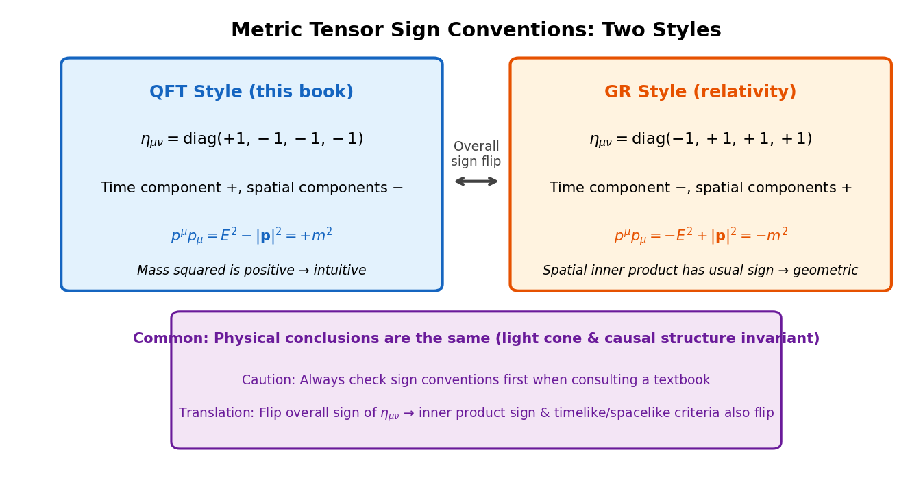
Fig. 2.1: Difference in sign conventions (QFT style vs. GR style). There are two sign conventions for the metric tensor: QFT style \((+,-,-,-)\) and GR style \((-,+,+,+)\). The physical conclusions are the same, but intermediate expressions differ in sign, so you must always check when consulting textbooks.
🔵 Kai: Sign conventions... In General Relativity General Relativity Ch. 4, we had \(\eta_{\mu\nu} = \text{diag}(-1, +1, +1, +1)\), right?
🟡 Lina: Yes. That's the GR style sign convention (mostly-plus, \((-,+,+,+)\)). However, in particle physics and quantum field theory textbooks, the opposite convention
—the QFT style (mostly-minus, \((+,-,-,-)\))—is standard. This book also adopts the QFT style.
⚪ Mei: Why are there two conventions?
🟡 Lina: Historical reasons. Both give the same physical conclusions, but several signs in intermediate expressions flip. Let me make a correspondence table.
Correspondence table between GR style \((-,+,+,+)\) and QFT style \((+,-,-,-)\)
| Quantity | GR style | QFT style (this book) |
|---|---|---|
| Metric | \(\eta_{\mu\nu} = \text{diag}(-1,+1,+1,+1)\) | \(\eta_{\mu\nu} = \text{diag}(+1,-1,-1,-1)\) |
| Spacetime interval | \(ds^2 = -dt^2 + d\mathbf{x}^2\) | \(ds^2 = dt^2 - d\mathbf{x}^2\) |
| Inner product of 4-momentum | \(p_\mu p^\mu = -m^2\) | \(p_\mu p^\mu = +m^2\) |
| Norm of 4-velocity (\(U^\mu = dx^\mu/d\tau\); see General Relativity General Relativity Ch. 4) | \(U_\mu U^\mu = -1\) | \(U_\mu U^\mu = +1\) |
| Timelike vector \(V\) | \(V_\mu V^\mu < 0\) | \(V_\mu V^\mu > 0\) |
| Spacelike vector \(V\) | \(V_\mu V^\mu > 0\) | \(V_\mu V^\mu < 0\) |
| Null (lightlike) vector | \(V_\mu V^\mu = 0\) | \(V_\mu V^\mu = 0\) (same) |
To translate formulas from General Relativity Chapters 3–4 to QFT style, flip the overall sign of \(\eta_{\mu\nu}\). This causes the sign of inner products and the "timelike/spacelike" convention to swap.
🔵 Kai: So \(p^\mu p_\mu = m^2\) with a positive sign is the QFT convention. Indeed, "mass squared is positive" is more intuitive...
🟡 Lina: Exactly. The QFT style has the advantage that "the time component is positive" and "the mass-shell condition \(p^\mu p_\mu = m^2\) is directly positive." On the other hand, the GR style has the advantage that "the spatial part of the metric is \(\eta_{ij} = +\delta_{ij}\), so the inner product of spatial vectors directly matches the \(\mathbf{A}\cdot\mathbf{B}\) you learned in high school." It's a matter of taste, so get into the habit of checking the sign convention first when consulting other textbooks—if you neglect this, the signs in intermediate expressions won't match and you'll get confused.
⚪ Mei: This book uses QFT style. When referring to General Relativity Chapters 3–4, watch the signs. Got it.
🟡 Lina: Exactly. Let me rewrite the formulas explicitly in QFT style.
Lowering the index gives
The time component stays the same, and the spatial components flip sign (opposite to GR style). The inner product of 4-vectors is
The mass-shell condition for 4-momentum is
✅ Comprehension Check: Under the QFT convention \(\eta_{\mu\nu} = \text{diag}(+1,-1,-1,-1)\), find \(A_\mu\) for the 4-vector \(A^\mu = (3, 1, 2, 0)\). Also compute \(A^\mu A_\mu\).
Answer
\(A_\mu = \eta_{\mu\nu} A^\nu = (3, -1, -2, 0)\) (time component unchanged, spatial components flip sign).
\(A^\mu A_\mu = A^0 A_0 + A^1 A_1 + A^2 A_2 + A^3 A_3 = 3 \cdot 3 + 1 \cdot (-1) + 2 \cdot (-2) + 0 \cdot 0 = 9 - 1 - 4 = 4\).
Since \(A^\mu A_\mu > 0\), this is a timelike vector in the QFT sign convention.
📝 Exercises:
- Raising/lowering indices, inner products, contractions → Problem B-1. Raising and Lowering Indices, Problem B-2. Inner Product of 4-Vectors, Problem B-3. Expanding the Einstein Summation Convention
2.3 Structure of the Lorentz Group
🟡 Lina: Now that we've organized the sign conventions, let's enter territory that is specific to quantum field theory. Up to here, the content overlapped with GR Ch.3–4, but from here on we're in new territory. We'll examine what structure the totality of Lorentz transformations possesses. In quantum field theory, it's this group structure that determines "what kinds of fields are allowed" and "what kinds of particles can exist."
General Definition of the Lorentz Transformation Matrix
🟡 Lina: A general Lorentz transformation acting on a 4-vector \(x^\mu\) is written as
\(\Lambda^\mu{}_\nu\) is a \(4 \times 4\) matrix called the Lorentz transformation matrix. Its defining property is "preserving the invariant interval"—for any \(x^\mu\), \(\eta_{\mu\nu}\, x'^\mu\, x'^\nu = \eta_{\mu\nu}\, x^\mu\, x^\nu\).
Let's work this out. Substituting \(x'^\mu = \Lambda^\mu{}_\alpha\, x^\alpha\) into the invariant interval condition gives
Since this must equal \(\eta_{\alpha\beta}\, x^\alpha\, x^\beta\) for any \(x^\alpha\), the contents of the parentheses themselves must be equal:
🔵 Kai: Since it "holds for any \(x\)," the parts that don't contain \(x\) must be equal to each other.
🟡 Lina: Exactly. In matrix form (defining the components of the matrix as \((\Lambda)^\mu{}_\nu = \Lambda^\mu{}_\nu\)),
Here \(\Lambda^T\) is the transpose matrix—rows and columns swapped (in ordinary matrix language, \((A^T)_{ij} = A_{ji}\), meaning the element in row \(i\), column \(j\) of the transpose equals the element in row \(j\), column \(i\) of the original matrix). Let me verify that (2.8) says the same thing as (2.7).
Let's confirm this concretely with a \(2 \times 2\) example. If we write the "row \(i\), column \(j\)" component of a matrix \(M\) as \(M^i{}_j\), then \(M = \begin{pmatrix} M^1{}_1 & M^1{}_2 \\ M^2{}_1 & M^2{}_2 \end{pmatrix}\). Note carefully—the superscript and subscript on \(M^i{}_j\) are just a convenient way to distinguish "row number and column number" and are separate from the contravariant/covariant distinction of tensors. However, for the Lorentz transformation matrix \(\Lambda^\mu{}_\nu\), since \(\Lambda\) is a matrix that "maps a contravariant vector \(x^\mu\) to another contravariant vector \(x'^\mu\)," the first index \(\mu\) (corresponding to the row number) is contravariant, and the second index \(\nu\) (corresponding to the column number) is covariant—so the matrix row/column distinction and the tensor contravariant/covariant distinction naturally coincide. That's why this notation works directly. The transpose \(M^T\) swaps rows and columns, so the "row \(i\), column \(j\)" component of \(M^T\) is the "row \(j\), column \(i\)" component of \(M\)—that is, \((M^T)^i{}_j = M^j{}_i\). Therefore \(M^T = \begin{pmatrix} M^1{}_1 & M^2{}_1 \\ M^1{}_2 & M^2{}_2 \end{pmatrix}\).
🔵 Kai: Ah, the diagonal components stay the same, and the off-diagonal components swap.
🟡 Lina: Right. Let's apply this to the \(4 \times 4\) Lorentz transformation matrix. The "row \(\mu\), column \(\nu\)" component of \(\Lambda\) is \(\Lambda^\mu{}_\nu\). Applying the transpose formula \((M^T)^i{}_j = M^j{}_i\), we get \((\Lambda^T)^\alpha{}_\mu = \Lambda^\mu{}_\alpha\)—meaning the "row \(\alpha\), column \(\mu\)" element of the transpose \(\Lambda^T\) is the "row \(\mu\), column \(\alpha\)" component \(\Lambda^\mu{}_\alpha\) of \(\Lambda\).
⚪ Mei: So, just like the \(2 \times 2\) example, swapping rows and columns gives \((\Lambda^T)^\alpha{}_\mu = \Lambda^\mu{}_\alpha\)—the row and column numbers are exchanged.
🔵 Kai: And then we use this to compute the components of the matrix product \(\Lambda^T \eta\, \Lambda\). How do you write the product of three matrices?
🟡 Lina: The same way as the ordinary matrix product \((AB)_{ij} = \sum_k A_{ik} B_{kj}\)—you contract over adjacent indices. For a product of three matrices \(ABC\), you can write it all at once as \((ABC)_{ij} = \sum_k \sum_l A_{ik} B_{kl} C_{lj}\)—whether you first compute \(AB\) and then multiply by \(C\), or multiply \(A\) by \(BC\), you get the same result.
Using this: the row \(\alpha\), column \(\beta\) component of \((\Lambda^T \eta\, \Lambda)\) is, by the definition of matrix multiplication, \(\sum_{\mu}\sum_{\nu}(\Lambda^T)^\alpha{}_\mu\, \eta_{\mu\nu}\, \Lambda^\nu{}_\beta\)—where we're writing the "row \(\mu\), column \(\nu\)" component of the matrix \(\eta\) as \(\eta_{\mu\nu}\) (simply expressing the matrix row/column numbers using tensor index notation). Substituting \((\Lambda^T)^\alpha{}_\mu = \Lambda^\mu{}_\alpha\) gives \(\sum_{\mu}\sum_{\nu}\Lambda^\mu{}_\alpha\, \eta_{\mu\nu}\, \Lambda^\nu{}_\beta\)—suppressing the \(\sum\) by Einstein's summation convention, this becomes \(\Lambda^\mu{}_\alpha\, \eta_{\mu\nu}\, \Lambda^\nu{}_\beta\). Setting this equal to \(\eta_{\alpha\beta}\) is precisely (2.7).
🔵 Kai: This is similar to how rotations satisfy \(R^T R = \mathbf{1}\). The identity matrix is just replaced by the metric \(\eta\).
🟡 Lina: Exactly. Rotations preserve \(\delta_{ij}\); Lorentz transformations preserve \(\eta_{\mu\nu}\). The structure is parallel. The "hyperbolic rotation" from General Relativity Ch. 3 is precisely this structure.
The Four Connected Components of the Lorentz Group
🟡 Lina: Now let's take the determinant of both sides of (2.8). I'll use two important properties of determinants. The first is "the determinant of a product of matrices equals the product of their determinants"—that is, \(\det(ABC) = \det A \cdot \det B \cdot \det C\). Intuitively, the determinant represents "by what factor a transformation stretches or shrinks volume," so the volume change factor for two successive transformations is the product of each transformation's volume change factor. You can verify this for the \(2 \times 2\) case: for \(A = \begin{pmatrix} a & b \\ c & d \end{pmatrix}\), \(\det A = ad - bc\), and indeed \(\det(AB) = \det A \cdot \det B\) can be confirmed by direct calculation (see also the cofactor expansion in General Relativity @chapter:gr/appendix_a). The second property is "the determinant is unchanged by transposition" (\(\det\Lambda^T = \det\Lambda\))—this can be proven from the fact that cofactor expansion (General Relativity @chapter:gr/appendix_a) gives the same value whether expanded along rows or columns. Intuitively, for the \(2 \times 2\) case: \(\det\begin{pmatrix} a & b \\ c & d \end{pmatrix} = ad - bc\), and the transpose gives \(\det\begin{pmatrix} a & c \\ b & d \end{pmatrix} = ad - cb = ad - bc\)—indeed the same. The general case works similarly.
🔵 Kai: I see—the product of volume change factors, and invariance under transposition—we use these two properties.
🟡 Lina: Using these two properties, the left side becomes \(\det(\Lambda^T \eta\, \Lambda) = \det\Lambda^T \cdot \det\eta \cdot \det\Lambda = (\det\Lambda)^2\, \det\eta\). The right side is \(\det\eta\). Since \(\det\eta = \det(\text{diag}(+1,-1,-1,-1)) = (+1)(-1)(-1)(-1) = -1 \neq 0\), dividing both sides by \(\det\eta\) gives
⚪ Mei: \(\det\Lambda\) can only be \(+1\) or \(-1\)—no intermediate values are possible.
🟡 Lina: Also, since (2.7) holds for any \(\alpha, \beta\), let's substitute \(\alpha = \beta = 0\) in particular:
Let me expand the left side using the QFT-style metric \(\eta_{\mu\nu} = \text{diag}(+1,-1,-1,-1)\). Since \(\mu\) and \(\nu\) each independently run from 0 to 3, there are nominally \(4 \times 4 = 16\) terms. But since \(\eta_{\mu\nu}\) is diagonal, \(\eta_{\mu\nu} = 0\) when \(\mu \neq \nu\)—so only the 4 terms with \(\mu = \nu\) survive:
Substituting \(\eta_{00} = +1\), \(\eta_{11} = \eta_{22} = \eta_{33} = -1\):
Rearranging:
(Equality holds when \(\Lambda^i{}_0 = 0\) (\(i = 1, 2, 3\))—that is, when all spatial-row components of the zeroth column of the transformation matrix vanish. The identity transformation and pure time reversal fall into this case.) A real number satisfying \(x^2 \geq 1\) must have \(|x| \geq 1\), meaning \(x \geq 1\) or \(x \leq -1\) (if \(|x| < 1\) then \(x^2 < 1\), a contradiction—think of the graph of \(y = x^2\) and the region where \(y \geq 1\)). Therefore \(\Lambda^0{}_0 \geq 1\) or \(\Lambda^0{}_0 \leq -1\). For example, the identity transformation (do nothing, \(\Lambda^\mu{}_\nu = \delta^\mu{}_\nu\)) has \(\Lambda^0{}_0 = 1\) (\(\det\Lambda = +1\)), and pure time reversal (\(t \to -t\), space unchanged, i.e., \(\Lambda = \text{diag}(-1, 1, 1, 1)\)) has \(\Lambda^0{}_0 = -1\) (the determinant of a diagonal matrix is the product of its diagonal elements, so \(\det\Lambda = (-1)(1)(1)(1) = -1\)).
✅ Comprehension Check: What are the two criteria used to classify the Lorentz transformation matrix \(\Lambda\) into four connected components? What values can each take?
Answer
(1) Whether \(\det\Lambda = +1\) or \(-1\), and (2) whether \(\Lambda^0{}_0 \geq 1\) or \(\Lambda^0{}_0 \leq -1\). The combinations of these divide the Lorentz group into four connected components. Since these values cannot jump under continuous parameter changes, it is impossible to continuously move between different connected components.
🔵 Kai: So the combinations of \(\det\Lambda = +1 / -1\) and \(\Lambda^0{}_0 \geq 1 / \leq -1\) split the Lorentz group into four parts. But what does "split" mean concretely? Why can't they mix?
🟡 Lina: Good question. Let me introduce the term connected component. A connected component is the collection of all transformations that can be reached by continuously and gradually varying the parameters (rotation angles, boost velocities). Why can't \(\det\Lambda\) or \(\Lambda^0{}_0\) jump midway? Because if you change the parameters gradually, the components of \(\Lambda\) also change gradually—meaning \(\det\Lambda\) and \(\Lambda^0{}_0\) are continuous functions, so to go from \(+1\) to \(-1\) you'd have to pass through \(0\) along the way. But every \(\Lambda\) along the path is also a Lorentz transformation matrix (satisfying condition (2.8)), so by (2.9), \(\det\Lambda = 0\) is impossible, and by (2.10), \(|\Lambda^0{}_0| < 1\) is also impossible. So jumping is impossible. Think of it as four islands separated by ocean—within the same island you can walk anywhere (= continuously vary parameters), but you can't swim to another island.
🔵 Kai: Ah, because you can't pass through "forbidden values" even by continuous changes, you can never reach a different island.
🟡 Lina: Let me explain the naming convention first. "Proper" means \(\det\Lambda = +1\) (preserves spatial orientation), and "orthochronous" means \(\Lambda^0{}_0 \geq 1\) (preserves the direction of time). "Improper" and "non-orthochronous" are their respective negations. With this naming convention in mind, look at Table 2.2 "The four connected components of the Lorentz group".
Table 2.2: The four connected components of the Lorentz group
| Connected component | Condition | Transformations included |
|---|---|---|
| Proper orthochronous \(L_+^\uparrow\) | \(\det\Lambda = +1\) and \(\Lambda^0{}_0 \geq 1\) | Ordinary rotations and boosts |
| Improper orthochronous \(L_-^\uparrow\) | \(\det\Lambda = -1\) and \(\Lambda^0{}_0 \geq 1\) | Includes parity \(P\) |
| Proper non-orthochronous \(L_+^\downarrow\) | \(\det\Lambda = +1\) and \(\Lambda^0{}_0 \leq -1\) | Includes \(PT\) (parity × time reversal) |
| Improper non-orthochronous \(L_-^\downarrow\) | \(\det\Lambda = -1\) and \(\Lambda^0{}_0 \leq -1\) | Includes time reversal \(T\) |
The overall picture is summarized in Fig. 2.2 "Structure of the Lorentz group and Poincaré group". This figure also shows the Poincaré group—obtained by adding spacetime translations (1 in the time direction + 3 in spatial directions = 4 parameters) to Lorentz transformations, for a total of 10 parameters—but we'll cover that in detail in 2.4 "The Poincaré Group—Lorentz Transformations + Spacetime Translations".
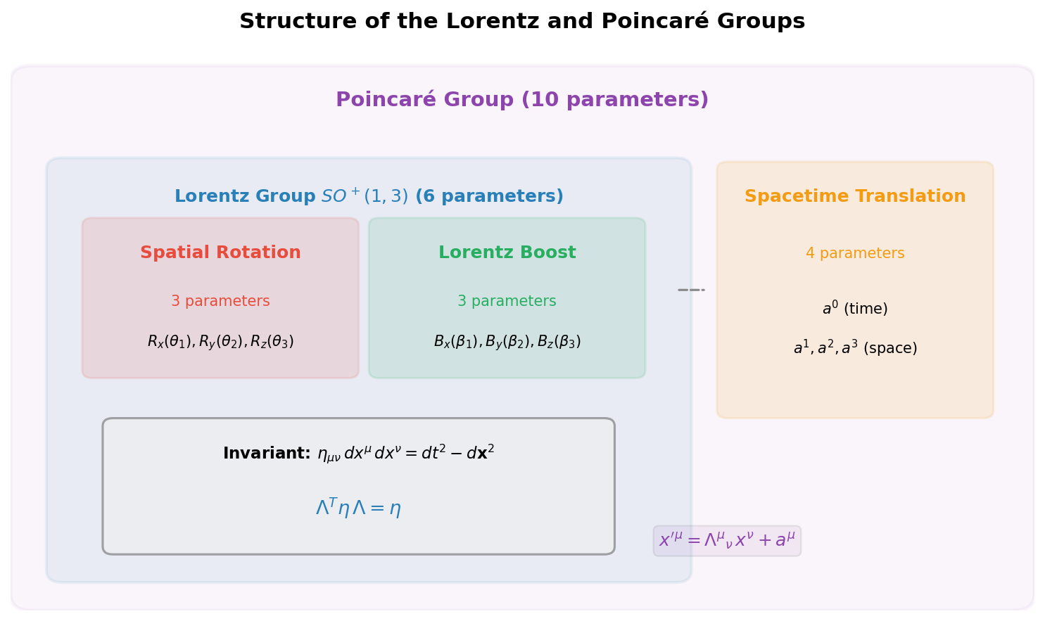
Fig. 2.2: Structure of the Lorentz group and Poincaré group. The Lorentz group splits into four connected components, and the proper orthochronous Lorentz group \(SO^+(1,3)\) is a continuous group with 3 rotations + 3 boosts = 6 parameters. The Poincaré group (10 parameters), obtained by adding 4 spacetime translation parameters, is explained in detail in 2.4 "The Poincaré Group—Lorentz Transformations + Spacetime Translations".
🟡 Lina: The most important for quantum field theory is the proper orthochronous Lorentz group \(SO^+(1,3)\) (\(L_+^\uparrow\))—the set of transformations that preserve both spatial orientation and the direction of time. Breaking down the notation: \(S\) stands for special (\(\det\Lambda = +1\)), \(O\) stands for a generalization of orthogonal—whereas the ordinary rotation group satisfies \(R^T R = \mathbf{1}\) (preserves the Euclidean metric \(\delta_{ij}\)), here we extend to \(\Lambda^T \eta\, \Lambda = \eta\) (preserves the Minkowski metric \(\eta_{\mu\nu}\))—\(+\) stands for orthochronous (preserves time direction), and \((1,3)\) indicates 1 time dimension and 3 space dimensions. \(SO^+(1,3)\) has 3 rotation parameters + 3 boost parameters = 6 parameters, and is a group with continuously varying parameters (a continuous group).
🔵 Kai: A "continuous group" is one like the rotation group where you can gradually change the angle, right? Does it have a special name?
🟡 Lina: It does. The definition of a group—closure, associativity, identity, inverse (the 4 conditions)—was covered in General Relativity General Relativity Ch. 4. In mathematics, among these, a group whose parameters can be varied continuously is called a Lie group. Concretely, when you change the rotation angle \(\theta\), the components of the rotation matrix \(\cos\theta\) and \(\sin\theta\) return finite values no matter how many times you differentiate with respect to \(\theta\), right? A Lie group is one where "when you change the transformation parameters, the matrix components change smoothly (can be differentiated any number of times)." For this chapter, you can think of it as essentially meaning "a group whose parameters can be continuously and gradually varied." Just remember the name—in references you'll frequently encounter the statement "the Lorentz group is a Lie group," and this terminology will also appear when we treat infinitesimal transformations in later chapters.
⚪ Mei: So in the same sense that the rotation group allows continuous variation of angles, the Lorentz group also allows continuous variation of parameters—that's why it's a Lie group.
🟡 Lina: Exactly. By the way, transformations with \(\det\Lambda = -1\) correspond to parity (spatial inversion) \(P\), and those with \(\Lambda^0{}_0 \leq -1\) correspond to time reversal \(T\). These cannot be continuously connected to \(SO^+(1,3)\)—they are discrete transformations.
🔵 Kai: Ah, the discrete symmetries we covered in Quantum Mechanics Quantum Mechanics Ch. 26! Parity violation, CP violation, and so on. But why are discrete transformations treated separately? What's fundamentally different from continuous transformations?
🟡 Lina: Using the "island" metaphor from before—continuous transformations are like walking around on the same island, while discrete transformations are like jumping to a different island—since you can't reach them by gradually varying parameters, you have no choice but to treat them as "separate things." And in quantum field theory, "whether \(P\) or \(T\) symmetry is violated" becomes an experimentally crucial question—P violation in weak interactions (1956, Lee-Yang) and CP violation (1964, Cronin-Fitch) are examples. We'll cover these in detail in later chapters.
⚪ Mei: So continuous transformations can move within the same connected component by varying parameters, but discrete transformations cross between connected components and can't be reached continuously—that's why they need to be treated as separate symmetries physically.
✅ Comprehension Check: How many continuous parameters does the proper orthochronous Lorentz group \(SO^+(1,3)\) have in total? Show the breakdown.
Answer
6 parameters. 3 spatial rotations (around the \(x, y, z\) axes) + 3 Lorentz boosts (in the \(x, y, z\) directions).
2.4 The Poincaré Group—Lorentz Transformations + Spacetime Translations
🟡 Lina: What's truly important in physics is not just the Lorentz group alone, but the group obtained by adding spacetime translations to it.
\(a^\mu\) is a constant 4-vector (the translation amount). The group formed by all such transformations is called the Poincaré group.
🔵 Kai: Translations have 4 parameters (\(a^0, a^1, a^2, a^3\)), and Lorentz transformations have 6 parameters, so together that's 10 parameters.
🟡 Lina: Exactly. And the fundamental requirement of quantum field theory is:
The equations of quantum field theory must not change form under transformations of the Poincaré group.
This requirement constrains the structure of the theory to a remarkable degree. Conversely, the starting difficulty from Quantum Mechanics Ch. 27—that "the Schrödinger equation is not Lorentz covariant"—can be avoided by requiring Poincaré invariance from the outset. In Quantum Mechanics Ch. 27, we noticed that "the existing equation isn't Lorentz covariant" and then groped toward the Klein-Gordon and Dirac equations, but in quantum field theory we use Poincaré invariance as a design principle from the start to construct equations—the order is reversed.
⚪ Mei: Instead of fixing things after the fact, you start from symmetry from the beginning.
🟡 Lina: In fact, Wigner (1939) took this perspective to its logical conclusion and converted the question "what is a particle in quantum field theory?" into a mathematical question.
🔵 Kai: You can get an answer to what a particle is using mathematics?
🟡 Lina: You can. The idea goes like this—if nature possesses Poincaré symmetry, then quantum mechanical states must "behave properly" under Poincaré transformations. That is, there must be definite rules for how quantum states change when you rotate or boost.
Let's first build intuition with a concrete example. When you rotate a vector \((v_x, v_y)\) in a 2D plane by angle \(\theta\),
Here we're associating a concrete matrix with the abstract operation of "rotation," right?
🔵 Kai: Yes, for each rotation angle there's exactly one matrix.
🟡 Lina: Right. Moreover, "rotating by \(30°\) then rotating by \(45°\)" gives the same result as "rotating by \(75°\)"—the property that the result of performing two transformations in succession matches the product of the corresponding matrices is preserved. A correspondence that preserves this property is called a representation. To put it more simply, a representation is "an assignment of one matrix to each element of the group (here, each rotation angle) such that the group multiplication (composition of transformations) is reproduced by matrix multiplication."
🔵 Kai: I see—you're having matrices act as "proxies" for the rotation operation. But what happens for operations other than rotations—for instance, what's the matrix for a scalar quantity?
🟡 Lina: Good question. Even for the same "rotation," if the object it acts on is different, the size and content of the matrix change. If acting on a 3D vector, it's a \(3 \times 3\) matrix; if acting on a scalar (just a number), it "does nothing" (the \(1 \times 1\) identity matrix). A scalar quantity like temperature doesn't change under rotation, so the corresponding "matrix" is just the number \(1\)—this is also a perfectly valid representation. In other words, for the same group, there can be multiple representations of different sizes.
⚪ Mei: The same group has different representations depending on "what it acts on"—\(2 \times 2\) for 2D plane vectors, \(3 \times 3\) for 3D vectors, \(1 \times 1\) for scalars.
🟡 Lina: Exactly. Let me also give you an intuitive sense of what "irreducible" means. Among representations, some "can actually be decomposed into a collection of smaller representations." Let me give a concrete example. Consider rotations in 3D space, and suppose we group together four quantities—temperature \(T\) and velocity vector \((v_x, v_y, v_z)\)—treating them as a 4-component vector. Under rotation, the 3 velocity components mix with each other, but temperature is a scalar so it doesn't change. That is, if we write the rotation matrix as \(4 \times 4\):
The upper-left \(1 \times 1\) block (temperature) and lower-right \(3 \times 3\) block (velocity) move independently without mixing, right? When a large matrix has this form—"an upper-left small square matrix and a lower-right small square matrix, with everything else (upper-right and lower-left) being zero"—we call it block diagonal. In this example, the \(4 \times 4\) representation decomposes into \(1 \times 1\) (scalar) and \(3 \times 3\) (vector)—this is a reducible representation. Conversely, the \(3 \times 3\) rotation matrix cannot be further split into smaller blocks no matter how you change the basis (i.e., no matter how you rotate the coordinate axes)—this is an irreducible representation, "the smallest indivisible unit." In chemistry terms, it's like decomposing molecules into atoms that can't be broken down further.
🔵 Kai: I see—like decomposing molecules into atoms. Irreducible = the smallest unit that can't be broken apart further.
🟡 Lina: And in quantum mechanics, the state of a physical system is represented by a "state vector" (see Quantum Mechanics). So with the same idea, we look for ways to express each Poincaré transformation (rotation, boost, translation) as a concrete operation "that changes quantum states in this way"—since if an observer rotates, the quantum state should change accordingly. And among these, "the smallest unit that cannot be decomposed further"—that is, the minimal set of states that mix with each other under any transformation—is called an irreducible representation. The key point here is that we're looking for "the minimal mixing set" under the entire Poincaré group including not just rotations but also boosts and translations—why this connects to the two labels of mass and spin will be explained after we see Wigner's result.
The answer Wigner found is surprisingly simple—let me state the conclusion first, then explain why. The result is summarized in Fig. 2.3 "Wigner's classification: correspondence between irreducible representations of the Poincaré group and particles".
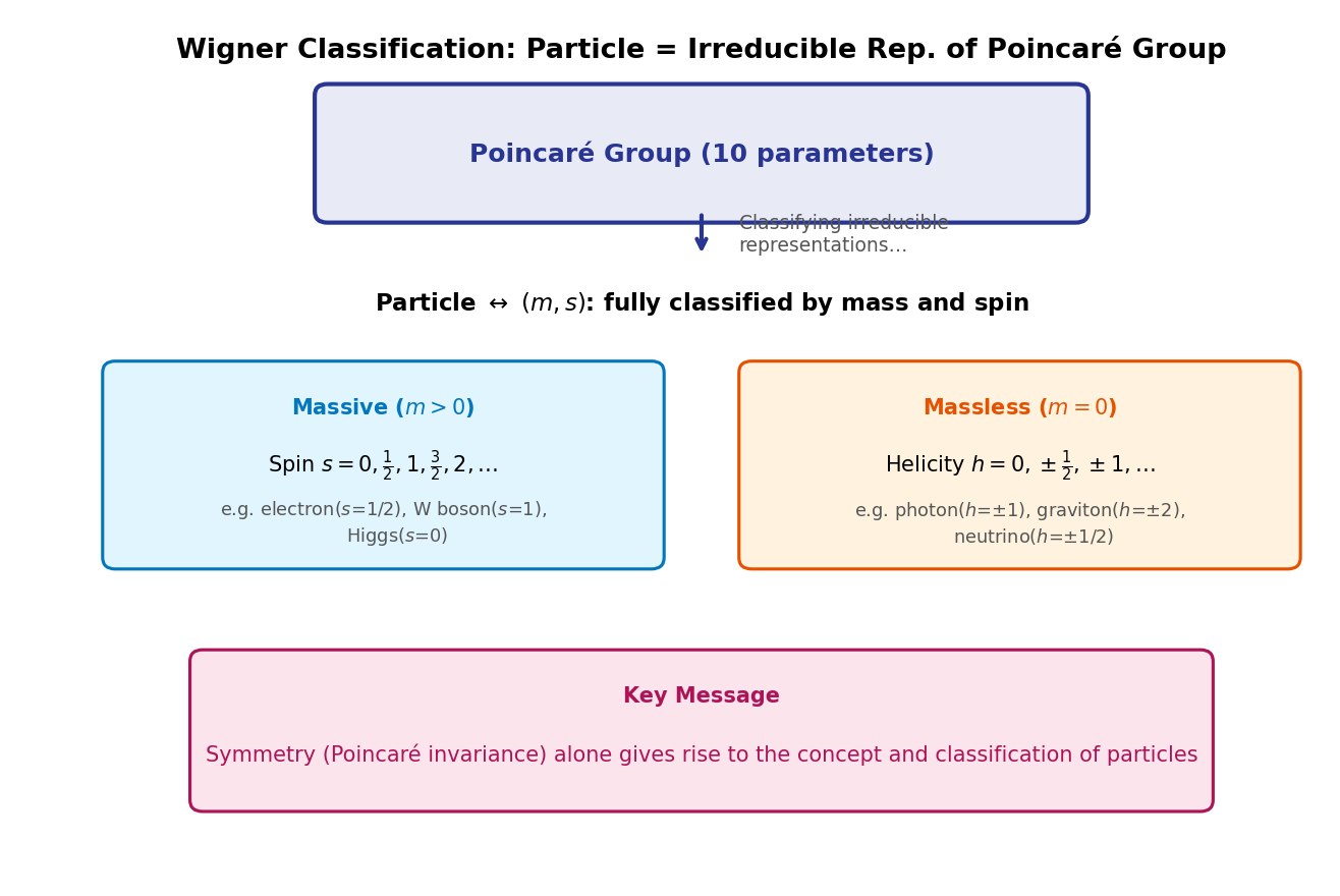
Fig. 2.3: Wigner's classification: correspondence between irreducible representations of the Poincaré group and particles. Particles are completely classified by just two labels (mass \(m\), spin \(s\)). The concept and classification of particles are derived from Poincaré symmetry alone.
Particle = irreducible representation of the Poincaré group (the smallest representation that cannot be decomposed further) = classified by labels (mass, spin)
The properties of a one-particle state are completely determined by just two numbers \((m, s)\). This is the result known as Wigner's classification. I'll explain "why just two suffice" shortly, in response to Kai's question. Specifically:
- \(m > 0\): spin \(s = 0, 1/2, 1, 3/2, \ldots\)
- \(m = 0\): helicity \(h = 0, \pm 1/2, \pm 1, \ldots\)
⚪ Mei: For the massless case it's "helicity" instead of "spin." What's the difference?
🟡 Lina: Helicity is the projection of spin onto the direction of motion—it represents "whether the spin points along or against the direction of travel." For a massive particle, an observer can overtake it, which reverses the "direction of motion," so helicity depends on the observer. But a massless particle travels at the speed of light and no one can overtake it—so helicity becomes an observer-independent invariant and can serve as a classification label instead of spin.
The detailed treatment is in Appendix B, but keep in mind the profound fact that "the concept of particles emerges from Poincaré symmetry alone."
✅ Comprehension Check: According to Wigner's classification, what labels classify particles in quantum field theory? And from which symmetry is this classification derived?
Answer
Particles are classified by two labels: (mass \(m\), spin \(s\)). This classification is derived from examining the irreducible representations of the Poincaré group. That is, the concept and classification of particles emerge from Poincaré symmetry (the symmetry of Lorentz transformations + spacetime translations) alone.
🔵 Kai: That's amazing... But I have two questions. First, I still don't quite get "irreducible representation." "The smallest unit that can't be decomposed further"—what does that look like concretely? Also, why are particles completely determined by just two quantities, mass and spin? It seems like there should be more quantum numbers needed...
🟡 Lina: Good questions. To build intuition for "irreducible," let me start with a simple example using just the rotation group. Consider a spin-\(1/2\) electron. There are two states: "spin up" and "spin down." When you rotate space, these two states mix with each other—in quantum mechanical language, they become superpositions. What was "spin up" becomes "a little bit up + a little bit down" as a superposition state. But no matter how you combine rotations, you never go outside these two states—a third state is never needed. So this set of two states is "the smallest indivisible unit" for the rotation group—an irreducible representation.
🔵 Kai: I see—the two states mix under rotation but remain closed within those two—that's "irreducible."
🟡 Lina: Right. But that's just an example for the rotation group alone. For the Poincaré group we must also include boosts and translations. Adding translations changes the momentum \(\mathbf{p}\), and boosts also change the momentum—so states with different momenta mix with each other.
🔵 Kai: Then won't states with all possible momenta get all mixed together, making classification impossible?
🟡 Lina: Good concern. But recall the mass-shell condition \(E^2 - |\mathbf{p}|^2 = m^2\). Under boosts and translations, \(E\) and \(\mathbf{p}\) change, but the combination \(m^2 = E^2 - |\mathbf{p}|^2\) is a Lorentz invariant and doesn't change. So "the collection of states with the same mass \(m\)" is closed under transformations. Furthermore, within that collection, the magnitude of spin \(s\) is also an invariant—boosts can change the direction of spin, but the magnitude of spin (\(s = 0, 1/2, 1, \ldots\)) doesn't change. As a result, "the collection of states with the same mass and same spin" forms one irreducible representation—that's why particles are classified by \((m, s)\).
🔵 Kai: So just by marrying relativity and quantum theory, you can determine what a particle is... But what about electric charge? Electrons and positrons have the same mass and spin but they're different particles, right?
🟡 Lina: Good point. Internal quantum numbers like electric charge or color charge come from symmetries separate from the Poincaré group (gauge symmetries). Wigner's classification tells us "the labels of particles determined by spacetime symmetry alone"—internal quantum numbers are additional information on top of that. We'll cover gauge symmetries in detail in later chapters.
🟡 Lina: Let me organize the argument so far. The logic of Wigner's classification is: (1) quantum states mix under Poincaré transformations → (2) mass \(m\) is a Lorentz invariant, so "states with the same \(m\)" are closed → (3) within those, behavior under rotations is determined by spin \(s\) → (4) ultimately \((m, s)\) becomes the label of the irreducible representation.
⚪ Mei: First you divide broadly by mass, then subdivide by spin—a two-stage classification.
🔵 Kai: So does that mean particles with spin \(3/2\) or \(2\) can exist in principle?
🟡 Lina: In principle, yes. In fact, spin-\(3/2\) particles (\(\Delta\) baryons, etc.) and spin-\(2\) particles (gravitons—if they exist) are known. As representations of the Poincaré group, any spin is allowed, but which ones are realized in nature is determined by the details of interactions—that's a topic for later chapters.
✅ Comprehension Check: Show that the number of parameters of the Poincaré group is 10, giving the breakdown by type of transformation.
Answer
3 spatial rotations (around the \(x, y, z\) axes) + 3 Lorentz boosts (in the \(x, y, z\) directions) + 4 spacetime translations (in the \(t, x, y, z\) directions) = 10 parameters total.
2.5 Lorentz Covariance and "Index Balance"
🟡 Lina: Now that we can see the Poincaré group—the symmetry that governs quantum field theory—let's come down to the practical matter of how to use it in everyday calculations. This is the technique of determining whether an equation is Lorentz covariant just by looking at the index positions. Once you master this, the hundreds of equations in subsequent chapters become dramatically easier to read.
Tensor Rank and Transformation Rules
🟡 Lina: We classify physical quantities by "how they transform under Lorentz transformations." This is a recap of what was done in General Relativity Ch. 4—summarized in Table 2.3 "Classification by tensor rank and transformation rules".
Table 2.3: Classification by tensor rank and transformation rules
| Name | Number of indices | Behavior under Lorentz transformation | Example |
|---|---|---|---|
| Scalar | 0 | Unchanged | Mass \(m\), invariant interval \(s^2\) |
| Vector | 1 | \(V^\mu \to \Lambda^\mu{}_\nu\, V^\nu\) | Position \(x^\mu\), momentum \(p^\mu\) |
| Rank-2 tensor | 2 | \(T^{\mu\nu} \to \Lambda^\mu{}_\alpha\, \Lambda^\nu{}_\beta\, T^{\alpha\beta}\) | Electromagnetic field \(F^{\mu\nu}\) |
A rank-\(n\) tensor gets \(n\) factors of \(\Lambda\)—this is the tensor transformation rule.
🔵 Kai: The more indices, the more complicated the transformation, but the pattern is the same. The number of \(\Lambda\)'s matches the number of indices.
The Requirement of Lorentz Covariance
🟡 Lina: Let me state the most important principle in quantum field theory in practical terms.
Field equations must be Lorentz covariant.
Concretely: The position and number of indices on both sides must match.
🔵 Kai: Both sides need to be the same kind of tensor, right?
🟡 Lina: Exactly. For example, if an equation has the form
then both sides are vectors. Under a Lorentz transformation, the same \(\Lambda^\mu{}_\nu\) acts on both sides, so if \(A^\nu = B^\nu\) holds, then \(A'^\mu = B'^\mu\) automatically holds too. The form of the equation is the same in every inertial frame. Conversely, if the left side were a vector and the right side a scalar, then under a Lorentz transformation only the left side would change while the right side wouldn't—such an equation would be physically meaningless.
⚪ Mei: In other words, an equation whose index types don't match breaks down the moment you change inertial frames.
🟡 Lina: In quantum field theory calculations, every time you write an equation you check whether "the number and position of indices match on both sides." This is index balance.
🔵 Kai: Index notation isn't just shorthand—it's a mechanism that automatically guarantees Lorentz covariance.
🟡 Lina: Precisely. This is the main reason for using index notation in quantum field theory. The key points of the judgment rules are summarized in Fig. 2.4 "Determining Lorentz covariance by index balance". The point is that indices paired up-and-down (contracted indices) disappear, and if the position and number of the remaining free indices match on both sides, the expression is Lorentz covariant—that's the basic judgment rule.
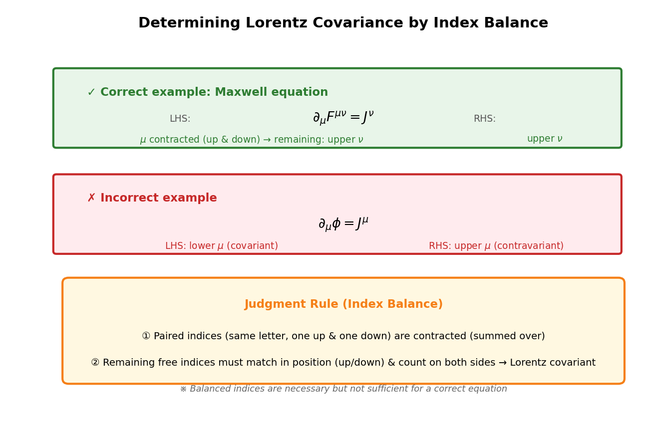
Fig. 2.4: Determining Lorentz covariance by index balance. Indices paired up and down are contracted and disappear; if the position and number of remaining free indices match on both sides, the expression is Lorentz covariant. Note that this is a necessary condition, not a sufficient one.
The d'Alembertian and the Klein-Gordon Equation
🟡 Lina: Let's do a concrete example. First, I'll define the differential operator as a 4-vector.
🔵 Kai: Wait, \(\partial_\mu\) has the index downstairs (covariant vector). Why is that?
🟡 Lina: Because it's a derivative with respect to \(x^\mu\) (upstairs). Let's see this explicitly. The Lorentz transformation is \(x'^\mu = \Lambda^\mu{}_{\nu}\, x^\nu\). Writing the inverse transformation—which recovers \(x\) from \(x'\)—as \(\Lambda^{-1}\), we have \(x^\nu = (\Lambda^{-1})^\nu{}_{\mu}\, x'^\mu\) (meaning that applying \(\Lambda\) then \(\Lambda^{-1}\) returns to the original). Here we use the multivariable chain rule. The single-variable chain rule you learned in high school is \(\frac{df}{dx} = \frac{df}{du}\frac{du}{dx}\). In the multivariable case, since \(f\) depends on \(x'^\mu\) through the 4 variables \(x^0, x^1, x^2, x^3\), you sum up contributions from all paths: \(\frac{\partial f}{\partial x'^\mu} = \frac{\partial x^0}{\partial x'^\mu}\frac{\partial f}{\partial x^0} + \frac{\partial x^1}{\partial x'^\mu}\frac{\partial f}{\partial x^1} + \cdots = \sum_\nu \frac{\partial x^\nu}{\partial x'^\mu}\frac{\partial f}{\partial x^\nu}\). This is the multivariable chain rule. The \(\frac{\partial}{\partial x^\mu}\) used here is the partial derivative—the operation of differentiating with respect to one variable while holding the others fixed (introduced in General Relativity General Relativity Ch. 4). The multivariable chain rule is the natural extension of partial derivatives.
🔵 Kai: You extend the single-variable chain rule to 4 variables and sum everything up.
🟡 Lina: Right. Now, \(x^\nu = (\Lambda^{-1})^\nu{}_{\mu}\, x'^\mu\) is a linear function of \(x'^\mu\) (\((\Lambda^{-1})^\nu{}_{\mu}\) is a constant), so differentiating with respect to \(x'^\mu\) gives \(\frac{\partial x^\nu}{\partial x'^\mu} = (\Lambda^{-1})^\nu{}_{\mu}\) (just like differentiating \(ax\) with respect to \(x\) gives \(a\)). Substituting this into the chain rule and treating \(f\) as an unspecified function to get an operator relation: \(\frac{\partial}{\partial x'^\mu} = (\Lambda^{-1})^\nu{}_{\mu}\frac{\partial}{\partial x^\nu}\) (with summation over \(\nu\)). So \(\partial_\mu\) gets acted on by the inverse matrix \(\Lambda^{-1}\), not \(\Lambda\). As we learned in General Relativity General Relativity Ch. 4, a contravariant vector (upper index) \(V^\mu\) transforms as \(V'^\mu = \Lambda^\mu{}_\nu V^\nu\) with \(\Lambda\), while a covariant vector (lower index) \(W_\mu\) transforms as \(W'_\mu = (\Lambda^{-1})^\nu{}_\mu W_\nu\) with \(\Lambda^{-1}\). \(\partial_\mu\) follows precisely this covariant vector transformation rule.
⚪ Mei: I see—\(\partial_\mu\) transforms with \(\Lambda^{-1}\), so it carries a lower index—it's a covariant vector.
🟡 Lina: Exactly. Intuitively, if you make the coordinate grid finer, coordinate values get larger but derivatives get smaller—the "inverse" of the transformation acts.
To raise the index we use the inverse metric \(\eta^{\mu\nu}\). For the Minkowski metric, \(\eta^{\mu\nu}\) is the inverse matrix of \(\eta_{\mu\nu}\). The inverse of a diagonal matrix is obtained by taking the reciprocal of each diagonal element (\(\text{diag}(a,b,c,d)^{-1} = \text{diag}(1/a, 1/b, 1/c, 1/d)\)), so \(1/(+1) = +1\), \(1/(-1) = -1\), giving \(\eta^{\mu\nu} = \text{diag}(+1,-1,-1,-1)\)—numerically the same as \(\eta_{\mu\nu}\). Using this:
The signs of the spatial derivatives flip (opposite to GR style). Using this, I'll define the d'Alembertian.
🔵 Kai: When you raise the index, the spatial components get a minus sign. In QFT style, the time component stays positive.
🟡 Lina: Summing over \(\mu = 0, 1, 2, 3\) by the contraction rule:
From (2.12) and (2.13), \(\partial^0 = \partial_0 = \frac{\partial}{\partial t}\), \(\partial^i = -\frac{\partial}{\partial x^i}\), \(\partial_i = \frac{\partial}{\partial x^i}\), so substituting each term:
That is, for the spatial components, the minus sign of \(\partial^i\) (from (2.13)) multiplied by the plus sign of \(\partial_i\) (from (2.12)) gives each spatial term a minus sign.
⚪ Mei: Time has a positive second derivative, space has negative second derivatives—exactly the same sign structure as the "spacetime interval \(ds^2 = dt^2 - d\mathbf{x}^2\)."
🟡 Lina: Note: In the General Relativity part of this book, General Relativity Ch. 19, we used the GR-style metric \((-,+,+,+)\) and defined \(\Box = \eta^{\mu\nu}\partial_\mu\partial_\nu\) (since \(\partial^\mu\partial_\mu = \eta^{\mu\nu}\partial_\mu\partial_\nu\), this means the same thing). In GR style, \(\eta^{00} = -1\), so \(\Box = -\partial^2/\partial t^2 + \nabla^2\). In this chapter's QFT style \((+,-,-,-)\), \(\eta^{00} = +1\), so the same definition \(\Box = \partial^\mu\partial_\mu\) gives \(\Box = \partial^2/\partial t^2 - \nabla^2\)—the sign is opposite. The same symbol \(\Box\) has different content depending on the metric sign convention—be careful. Also, some textbooks define \(\Box \equiv -\eta^{\mu\nu}\partial_\mu\partial_\nu\) (in GR style) by including a minus sign in the definition itself, so that \(\Box = \partial^2/\partial t^2 - \nabla^2\) regardless of which metric convention is used. Always check the sign convention when consulting other textbooks.
🔵 Kai: \(\partial^\mu \partial_\mu\) has the same index contracted up and down. Does that make it a scalar?
🟡 Lina: Exactly. Contracting the same index up and down makes it disappear, producing a Lorentz scalar—the same mechanism as \(A^\mu B_\mu\) being a scalar. So \(\Box = \partial^\mu \partial_\mu\) is automatically a Lorentz scalar operator. A scalar operator acting on a scalar field \(\phi\) produces a result that's still a scalar—since no indices are added or removed.
⚪ Mei: So the operator \(\Box\) with all indices contracted away is a scalar operator, and acting on a scalar field \(\phi\) doesn't add any indices—therefore \(\Box\phi\) is also a scalar. You can determine the transformation property just by counting indices.
🟡 Lina: Exactly. The Klein-Gordon equation is
🔵 Kai: In Quantum Mechanics Ch. 27 it was written as
Is that the same as (2.15) here? Where did \(c\) and \(\hbar\) go...?
🟡 Lina: Try substituting natural units \(c = \hbar = 1\).
🔵 Kai: Let's see, putting \(c = 1\) makes \(1/c^2 = 1\) so the first term becomes \(\frac{\partial^2 \phi}{\partial t^2}\), and putting \(\hbar = 1\) makes \(m^2 c^2/\hbar^2 = m^2\) so... \(\frac{\partial^2 \phi}{\partial t^2} - \nabla^2 \phi + m^2 \phi = 0\). Oh, that's exactly \((\Box + m^2)\phi = 0\)!
⚪ Mei: Just switching to natural units makes that long equation this compact.
🟡 Lina: That's the power of natural units + index notation. Looking at (2.15), both sides are scalars (\(\Box\) and \(m^2\) are scalar operators, \(\phi\) is a scalar field, and 0 is a scalar). The index balance is satisfied → automatically Lorentz covariant—you can judge this at a glance.
Practice: Checking Index Balance
🟡 Lina: Let's look at several equations and determine Lorentz covariance by checking index balance.
Example 1: Maxwell's equations
Left side: \(\partial_\mu\) has lower \(\mu\), \(F^{\mu\nu}\) has upper \(\mu, \nu\). \(\mu\) is contracted up-down and disappears, leaving one upper \(\nu\). Right side: \(J^\nu\) also has one upper \(\nu\). → Both sides are the same kind of 4-vector → Lorentz covariant ✓
Example 2: An incorrect equation
Left side: one lower \(\mu\) (covariant vector). Right side: one upper \(\mu\) (contravariant vector). → Index positions don't match → Not Lorentz covariant ✗
🔵 Kai: Wow, you can determine it just by looking at whether indices are up or down! But if the index balance is satisfied, does that necessarily mean it's a correct physical equation? There could be equations with balanced indices that are physically wrong, right?
🟡 Lina: Sharp. Index balance is a necessary condition but not a sufficient one. An equation with unbalanced indices is definitely wrong. But even if the balance holds, if the coefficients or signs are wrong, it's not physically correct. Think of index balance as "a filter that catches obvious mistakes."
✅ Comprehension Check: Is having balanced indices a sufficient condition or a necessary condition for an equation to be Lorentz covariant? Briefly explain why.
Answer
It is a necessary condition but not a sufficient one. If index balance fails, the equation is definitely not Lorentz covariant, but even with balanced indices, the equation may not be physically correct if coefficients or signs are wrong. Index balance functions as "a filter that catches obvious mistakes."
🟡 Lina: Right. Hundreds of equations will appear from now on, but just by checking "are the indices balanced?" you can prevent many calculation errors. It's a technique you'll use for the rest of your life in quantum field theory.
✅ Comprehension Check: Determine whether the following equation is Lorentz covariant by checking index balance: \(T^{\mu\nu} = \partial^\mu \phi\, \partial^\nu \phi - \eta^{\mu\nu}\left(\frac{1}{2}\partial_\alpha \phi\, \partial^\alpha \phi - \frac{1}{2}m^2 \phi^2\right)\)
Answer
Left side: two upper free indices \(\mu, \nu\) → rank-2 contravariant tensor. Right side, first term: \(\partial^\mu \phi\) has upper \(\mu\), \(\partial^\nu \phi\) has upper \(\nu\) → the product is a rank-2 tensor with upper \(\mu, \nu\). Right side, second term: \(\eta^{\mu\nu}\) has upper \(\mu, \nu\); inside the parentheses, \(\alpha\) is contracted up-down making it a scalar, and \(\phi^2\) is also a scalar → overall has upper \(\mu, \nu\) as a rank-2 tensor. Both sides have upper \(\mu, \nu\) as rank-2 contravariant tensors, so it is Lorentz covariant ✓.
📝 Exercises:
- Conditions on Lorentz transformation matrices, transformation of the electromagnetic field tensor → Problem M-1. Derivation of the Condition on the Lorentz Transformation Matrix, Problem A-1. Transformation Rules for Contravariant and Covariant Tensors, and Application to the Electromagnetic Field Tensor
2.6 Three Requirements for Quantum Field Theory
🟡 Lina: At the end of this chapter, let's organize the three requirements that form the foundation of quantum field theory. The overall picture is illustrated in Fig. 2.5 "The three requirements of quantum field theory and the spin-statistics theorem".
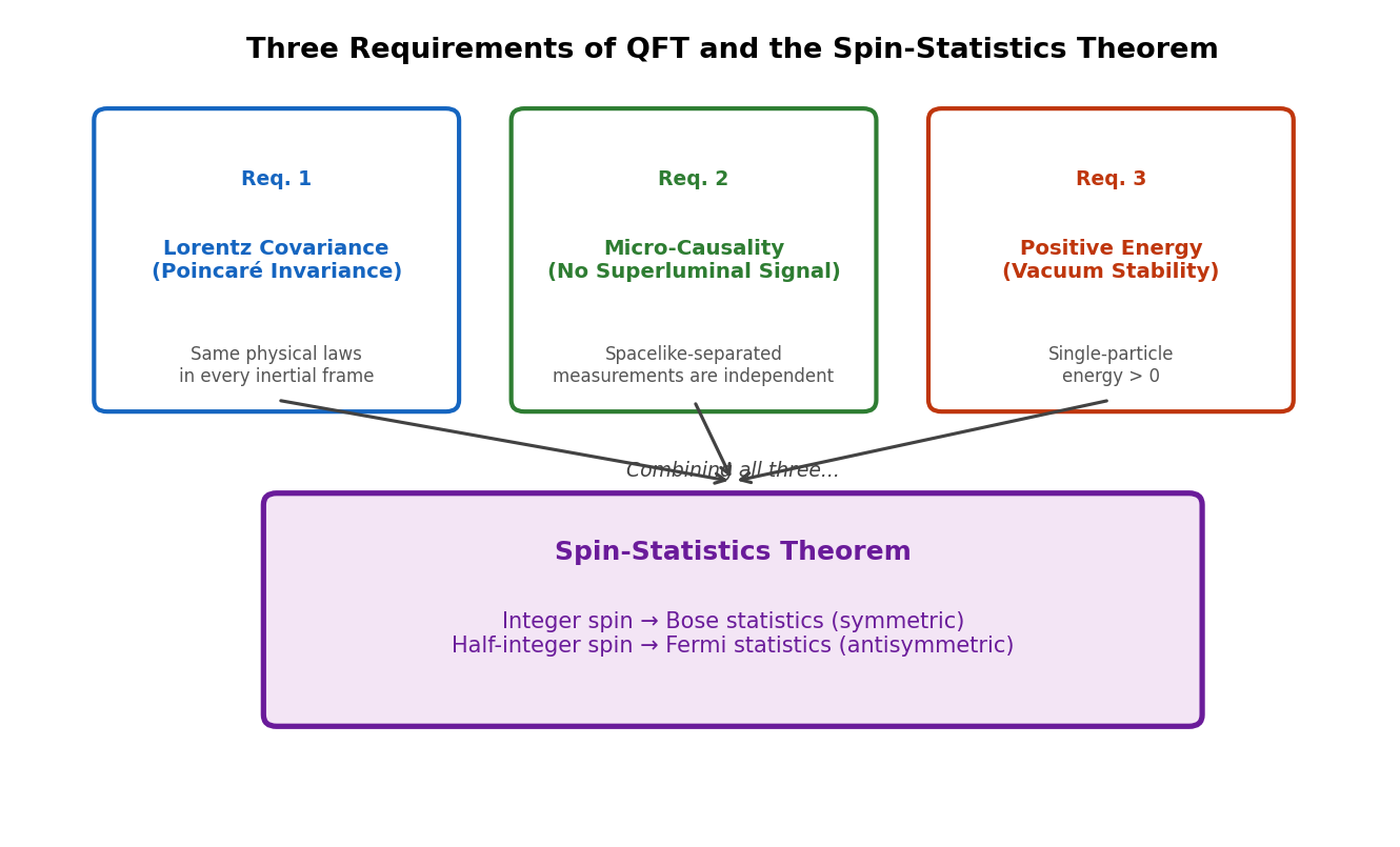
Fig. 2.5: The three requirements of quantum field theory and the spin-statistics theorem. Combining the three requirements of Lorentz covariance, microcausality, and positive energy leads to the spin-statistics theorem (integer spin → Bose statistics, half-integer spin → Fermi statistics).
- Lorentz covariance (Poincaré invariance): The field equations don't change form under Poincaré group transformations
- Causality (microcausality): Information cannot travel faster than light. Measurement results at two points outside each other's light cone—that is, two points so far apart that even light cannot travel from one to the other (see General Relativity General Relativity Ch. 3)—must be independent of each other. Intuitively, this means "experiments performed simultaneously at two sufficiently separated locations cannot influence each other." The precise formulation of this in the mathematics of quantum theory will be introduced in a later chapter
- Positive energy: The energy of physical one-particle states is positive (the vacuum is stable)
🔵 Kai: For the causality part, "measurement results at points outside the light cone are independent of each other"—could you be a bit more concrete about what that means?
🟡 Lina: For example, suppose you perform an experiment in Tokyo right now, and another experiment is performed in the Andromeda galaxy—if the two events are spacelike separated (even light can't get from one to the other), then the Tokyo experiment cannot possibly influence the Andromeda experiment. No matter what operation you perform in Tokyo, the statistics of the Andromeda experiment (which values appear with what frequency) don't change at all. And vice versa. That's the intuitive meaning of causality.
⚪ Mei: Even with quantum entanglement (Quantum Mechanics Quantum Mechanics Ch. 23), only correlations are visible and no information can be sent—the same spirit.
🟡 Lina: You might think "But wait, with quantum entanglement (Quantum Mechanics Quantum Mechanics Ch. 23), weren't there correlations between distant particles?" But as we confirmed then, looking at one side's data alone it appears random—correlations only become visible when you compare both datasets together. So you can't change the other side's statistics by operating on one side (no-signaling). Causality is preserved in this sense. The precise formulation in quantum theory—specifically, the condition that "field operators at spacelike separated points commute"—will be introduced in a later chapter.
🔵 Kai: I see. So do these three requirements determine the form of the theory pretty tightly?
🟡 Lina: To a remarkable degree. From Lorentz covariance (more precisely, Poincaré invariance) alone, Wigner's classification discussed in 2.4 "The Poincaré Group—Lorentz Transformations + Spacetime Translations" emerges—"fields are classified by (mass, spin)." Furthermore, combining causality with positive energy allows one to prove the spin-statistics theorem:
Integer-spin fields → Bose statistics; half-integer-spin fields → Fermi statistics
🔵 Kai: Wait—the distinction between bosons and fermions comes out of just three requirements?!
✅ Comprehension Check: From which three requirements of quantum field theory is the spin-statistics theorem derived? Also, briefly explain what this theorem states.
Answer
It is derived from the three requirements of (1) Lorentz covariance (Poincaré invariance), (2) causality (microcausality), and (3) positive energy (vacuum stability). The theorem states that "integer-spin fields obey Bose statistics and half-integer-spin fields obey Fermi statistics." The distinction between bosons and fermions, which was assumed axiomatically in quantum mechanics, can be proven from these three principles in quantum field theory.
⚪ Mei: So in quantum mechanics, "electrons are fermions, photons are bosons" was assumed axiomatically, but in quantum field theory it's derivable from those three requirements.
🟡 Lina: Yes. This is one of the most dramatic examples of "symmetry determines physics." Starting from the next chapter, we'll use this Lorentz covariance as a weapon to study classical field theory—Lagrangians and Noether's theorem.
🔵 Kai: The spin-statistics theorem comes from just three requirements... But honestly, I can't yet imagine what the proof looks like.
🟡 Lina: The proof requires the tool of field commutation relations, so we'll revisit it in a later chapter after learning that. Look forward to it.
🔵 Kai: I'm looking forward to it. ...Oh, can I go back to the discussion in 2.5 "Lorentz Covariance and "Index Balance""? You said earlier that index balance is "a necessary condition but not sufficient." Isn't that similar to dimensional analysis? The same feeling as "even if the dimensions match, the equation isn't necessarily correct."
🟡 Lina: Good intuition. Exactly—just as dimensional analysis catches obvious mistakes through "unit balance," index checking catches mistakes through "Lorentz transformation balance." Both are necessary-condition filters, not sufficient conditions. Your analogy is precise.
🔵 Kai: So even if an equation passes both filters, it could still be wrong—what's the ultimate basis for judging it "correct"?
🟡 Lina: There are two. One is agreement with experiment—ultimately nature holds the answer. The other is logical derivation from the action principle—being able to trace back to principles explaining "why this equation." Filters are just tools for "catching obvious mistakes"; the guarantee of correctness lies elsewhere—and that's the role of the Lagrangian, which we'll learn in the next chapter. In other words, you use the index check to eliminate "obviously wrong" expressions, then from what remains you use the action principle to select "the correct one"—it's a two-stage process.
⚪ Mei: Use filters to drop "the bad ones," then use principles to select "the right one"—a two-stage mechanism.
🔵 Kai: I see. So in the next chapter on Lagrangians, you start from a scalar quantity with balanced indices and derive equations from there?
🟡 Lina: Exactly right. The Lagrangian must be a scalar—the index balance we learned today becomes the design guideline when constructing Lagrangians in the next chapter. Using the tools acquired in this chapter—the QFT sign convention, the structure of the Lorentz group and Poincaré group, and covariance checking via index balance—in the next chapter we'll finally move to the side of "deriving" field equations.
🔵 Kai: Deriving equations from symmetry—until now we started with equations and checked their symmetry, but now it reverses. I'm excited.
Preview of the Next Chapter
Ch. 3 Classical Field Theory — Lagrangians and Noether's Theorem
In the next chapter, we learn a systematic method for deriving Lorentz-covariant field equations. The keys are the Lagrangian (action principle) and Noether's theorem—the profound theorem that "every continuous symmetry implies a conserved quantity." We'll see how the Klein-Gordon field and electromagnetic field equations are both derived from a single Lagrangian.
References
- Quantum Field Theory and the Standard Model (Schwartz) Chapter 2, "Lorentz invariance and second quantization"
- Quantum Field Theory for the Gifted Amateur (Lancaster & Blundell) Chapter 10, "Transformations"
- Sakamoto Masato, Quantum Field Theory — Focusing on Invariance and Free Fields Chapter 1, "Invitation to quantum field theory"; Chapter 14, "Poincaré algebra and classification of one-particle states"
- Quantum Field Theory (David Tong lecture notes) Chapter 1, "Classical Field Theory" (introductory part)
- Wigner, E. P. "On Unitary Representations of the Inhomogeneous Lorentz Group," Ann. Math. 40, 149 (1939) (original paper on Wigner's classification)
- Lee, T. D. and Yang, C. N. "Question of Parity Conservation in Weak Interactions," Phys. Rev. 104, 254 (1956)
- Christenson, J. H., Cronin, J. W., Fitch, V. L. and Turlay, R. "Evidence for the \(2\pi\) Decay of the \(K_2^0\) Meson," Phys. Rev. Lett. 13, 138 (1964)
Feedback on this page
Let us know if something was unclear, incorrect, or could be improved.