Chapter 1: Why Quantum Field Theory Is Needed — Continuing from Quantum Mechanics Ch. 27

← Welcome to This JourneyCh. 2 Review of Special Relat… →

Story so far:

In Quantum Mechanics Ch. 27, we discovered that the Schrödinger equation contradicts special relativity, derived the Klein-Gordon and Dirac equations, saw the prediction of antiparticles, and gained the perspective that quantum field theory (QFT) is needed to describe "phenomena where the number of particles changes."

Goals of This Chapter

• Understand "why a single-particle wave function is insufficient" from 3 independent arguments, and establish the Quantum Field Theory worldview that "particles are excitations of fields"
• Introduce the concept of Fock space and gain an overview of the entire Quantum Field Theory

---

1.1　The Endpoint of Quantum Mechanics Ch. 27 — Confirming Our Starting Point

🟡 Lina: Welcome back. In the final chapter of quantum mechanics, Quantum Mechanics Ch. 27, we made it quite far. Let's briefly review where we ended up.

🔵 Kai: Um, since the Schrödinger equation doesn't work with relativity, we used the relativistic energy relation \(E^2 = p^2c^2 + m^2c^4\) to construct the Klein-Gordon equation, right?

⚪ Mei: And the Klein-Gordon equation had the problem that "the probability density can become negative." To solve this, Dirac created a first-order equation, from which the existence of antiparticles was predicted.

🟡 Lina: Exactly. And finally, Quantum Mechanics Ch. 27 ended with the perspective that "to describe phenomena where particle number changes, we need to quantize the field itself rather than working with wave functions." Today, we'll flesh out that perspective more concretely, using equations.

🔵 Kai: "Quantize the field" — honestly, I still don't quite get it...

🟡 Lina: Don't worry. By the end of this chapter, "why we must do this" should click into place. First, let's trace through the difficulties of the Klein-Gordon equation more carefully with equations than we did in Quantum Mechanics Ch. 27.

---

1.2　Difficulties of the Klein-Gordon Equation — Breakdown of the Probability Interpretation

Review of the Equation

🟡 Lina: Let me write down the Klein-Gordon equation that we derived in Quantum Mechanics Ch. 27. Using natural units \(\hbar = c = 1\):

\[ \frac{\partial^2 \phi}{\partial t^2} - \nabla^2 \phi + m^2 \phi = 0 \tag{1.1} \]

Writing \(c\) and \(\hbar\) explicitly:

\[ \frac{1}{c^2}\frac{\partial^2 \phi}{\partial t^2} - \nabla^2 \phi + \frac{m^2 c^2}{\hbar^2}\phi = 0 \tag{1.2} \]

🔵 Kai: This was obtained by replacing both sides of \(E^2 = p^2c^2 + m^2c^4\) with operators, right?

🟡 Lina: That's right. And as we confirmed in Quantum Mechanics Ch. 27, since time and space are treated symmetrically through second-order derivatives, Lorentz covariance is satisfied. But Lorentz covariance is a necessary condition, not a sufficient one.

🔵 Kai: Not sufficient — meaning there are other conditions that need to be satisfied?

🟡 Lina: Yes. In the Schrödinger equation, the probability density \(\rho = |\psi|^2\) was guaranteed to always be non-negative, right? We need to check whether the same holds for the Klein-Gordon equation. Let's calculate it.

The Continuity Equation and Probability Density

🟡 Lina: For probability to be conserved in quantum mechanics, the probability density \(\rho\) and probability current density \(\mathbf{j}\) must satisfy the continuity equation:

\[ \frac{\partial \rho}{\partial t} + \nabla \cdot \mathbf{j} = 0 \tag{1.3} \]

We confirmed in Quantum Mechanics Ch. 7 that this holds with \(\rho = |\psi|^2\) for the Schrödinger equation. Let's try the same thing for the Klein-Gordon equation.

🟡 Lina: We multiply Eq. (1.1) from the left by \(\phi^*\), and multiply the complex conjugate of Eq. (1.1) from the left by \(\phi\), then take their difference. Let me work through this explicitly.

The complex conjugate of Eq. (1.1) is:

\[ \frac{\partial^2 \phi^*}{\partial t^2} - \nabla^2 \phi^* + m^2 \phi^* = 0 \tag{1.4} \]

Computing "\(\phi^*\) × Eq. (1.1)" \(-\) "\(\phi\) × Eq. (1.4)":

\[ \phi^* \frac{\partial^2 \phi}{\partial t^2} - \phi \frac{\partial^2 \phi^*}{\partial t^2} - \phi^* \nabla^2 \phi + \phi \nabla^2 \phi^* = 0 \]

🔵 Kai: The \(m^2\) terms cancel since \(\phi^* m^2 \phi - \phi m^2 \phi^* = 0\), right?

🟡 Lina: Exactly. Let's organize the remaining terms. Writing the difference again:

\[ \phi^* \frac{\partial^2 \phi}{\partial t^2} - \phi \frac{\partial^2 \phi^*}{\partial t^2} - \phi^* \nabla^2 \phi + \phi \nabla^2 \phi^* = 0 \]

The time derivative part:

\[ \phi^* \frac{\partial^2 \phi}{\partial t^2} - \phi \frac{\partial^2 \phi^*}{\partial t^2} = \frac{\partial}{\partial t}\left(\phi^* \frac{\partial \phi}{\partial t} - \phi \frac{\partial \phi^*}{\partial t}\right) \]

The spatial derivative part (paying attention to signs):

\[ -\phi^* \nabla^2 \phi + \phi \nabla^2 \phi^* = -(\phi^* \nabla^2 \phi - \phi \nabla^2 \phi^*) = -\nabla \cdot \left(\phi^* \nabla \phi - \phi \nabla \phi^*\right) \]

(The last equality can be verified by expanding \(\nabla \cdot (\phi^* \nabla \phi) = (\nabla \phi^*) \cdot (\nabla \phi) + \phi^* \nabla^2 \phi\), doing the same for the other term, and subtracting — the \((\nabla \phi^*) \cdot (\nabla \phi)\) terms cancel, confirming \(\phi^* \nabla^2 \phi - \phi \nabla^2 \phi^* = \nabla \cdot (\phi^* \nabla \phi - \phi \nabla \phi^*)\).)

⚪ Mei: Both use the product rule of differentiation in reverse.

🔵 Kai: Um, for example, for the time derivative part: \(\frac{\partial}{\partial t}\left(\phi^* \frac{\partial \phi}{\partial t}\right) = \frac{\partial \phi^*}{\partial t}\frac{\partial \phi}{\partial t} + \phi^* \frac{\partial^2 \phi}{\partial t^2}\), and expanding the other one similarly and subtracting... indeed the \(\frac{\partial \phi^*}{\partial t}\frac{\partial \phi}{\partial t}\) terms cancel and we get back the left side. But why do we do this operation? "Multiply by \(\phi^*\) and subtract" seems like it comes out of nowhere...

🟡 Lina: Good question. This is actually the exact same technique we used to show probability conservation for the Schrödinger equation (recall Quantum Mechanics Ch. 7). Back then, we also computed \(\psi^*\) × equation \(-\) \(\psi\) × complex conjugate equation to derive the continuity equation, right? "When you want to find a conserved quantity, multiply by the complex conjugate and subtract" is a standard trick. The spatial derivative part has exactly the same structure.

🟡 Lina: Putting it together:

\[ \frac{\partial}{\partial t}\left(\phi^* \frac{\partial \phi}{\partial t} - \phi \frac{\partial \phi^*}{\partial t}\right) - \nabla \cdot \left(\phi^* \nabla \phi - \phi \nabla \phi^*\right) = 0 \]

We want to organize this into the form of the continuity equation \(\frac{\partial \rho}{\partial t} + \nabla \cdot \mathbf{j} = 0\). First, let's multiply the whole thing by \(\frac{i}{2m}\). Why \(i\) is needed: \(\phi^* \frac{\partial \phi}{\partial t} - \phi \frac{\partial \phi^*}{\partial t}\) is actually purely imaginary (for any complex number \(z\), \(z - z^*\) is always purely imaginary, right? It has the same structure). So we need to multiply by \(i\) to make it real. The result is:

\[ \frac{\partial}{\partial t}\underbrace{\left[\frac{i}{2m}\left(\phi^* \frac{\partial \phi}{\partial t} - \phi \frac{\partial \phi^*}{\partial t}\right)\right]}_{\equiv\,\rho} - \nabla \cdot \left[\frac{i}{2m}\left(\phi^* \nabla \phi - \phi \nabla \phi^*\right)\right] = 0 \]

🔵 Kai: Ah, the content of the brackets under the time derivative becomes \(\rho\), and we read off \(\mathbf{j}\) from the spatial derivative term.

🟡 Lina: Exactly. Now compare with the continuity equation \(\frac{\partial \rho}{\partial t} + \nabla \cdot \mathbf{j} = 0\). It's natural to define the content of the brackets under the time derivative as \(\rho\) (that's what the \(\underbrace{\cdots}_{\equiv\,\rho}\) in the equation indicates). The spatial derivative term has the form \(-\nabla \cdot (\cdots)\), so to get \(+\nabla \cdot \mathbf{j}\), we just need to define \(\mathbf{j} = -\frac{i}{2m}(\phi^* \nabla \phi - \phi \nabla \phi^*)\). We're just absorbing the minus sign into the definition of \(\mathbf{j}\).

🔵 Kai: Um, I'm getting a bit confused with the signs... Looking at the equation after multiplying by \(\frac{i}{2m}\), the spatial derivative term is \(-\frac{i}{2m}\nabla \cdot (\phi^* \nabla \phi - \phi \nabla \phi^*)\), right? The continuity equation has \(+\nabla \cdot \mathbf{j}\), so if we define \(\mathbf{j} = -\frac{i}{2m}(\phi^* \nabla \phi - \phi \nabla \phi^*)\), it all works out?

🟡 Lina: Exactly. So the full equation after multiplying by \(\frac{i}{2m}\) is:

\[ \frac{\partial \rho}{\partial t} \underbrace{- \frac{i}{2m}\nabla \cdot (\phi^* \nabla \phi - \phi \nabla \phi^*)}_{= +\nabla \cdot \mathbf{j}} = 0 \]

So by defining \(\mathbf{j} = -\frac{i}{2m}(\phi^* \nabla \phi - \phi \nabla \phi^*)\), it fits perfectly into the continuity equation form.

🔵 Kai: OK, so we absorb the minus sign from the original equation into the definition of \(\mathbf{j}\) to get the \(+\nabla \cdot \mathbf{j}\) form. But why \(\frac{i}{2m}\)? It seems to come out of nowhere...

🟡 Lina: Good question. Note that here we're using natural units \(\hbar = c = 1\), which is why the coefficient is \(\frac{i}{2m}\). If we write \(\hbar\) and \(c\) explicitly, the coefficient for \(\rho\) becomes \(\frac{i\hbar}{2mc^2}\) (while for \(\mathbf{j}\) it's \(-\frac{i\hbar}{2m}\) — note that \(\rho\) has an extra factor of \(c^2\) in the denominator compared to \(\mathbf{j}\). This difference comes from the \(1/c^2\) multiplying the time derivative in Eq. (1.2) — if you perform the same procedure "\(\phi^*\) × Eq. (1.2)" \(-\) "\(\phi\) × complex conjugate" you'll find the time derivative terms carry an extra \(1/c^2\), which puts \(c^2\) in the denominator of \(\rho\)'s coefficient). Let me elaborate on why \(i\) is needed. For a complex number \(z = a + bi\), we have \(z - z^* = (a+bi) - (a-bi) = 2bi\), which is purely imaginary. Now consider the quantity \(\phi^* \frac{\partial \phi}{\partial t}\) — its complex conjugate is \((\phi^* \frac{\partial \phi}{\partial t})^* = \phi \frac{\partial \phi^*}{\partial t}\) (taking the conjugate turns \(\phi^* \to \phi\) and \(\frac{\partial \phi}{\partial t} \to \frac{\partial \phi^*}{\partial t}\)). So \(\phi^* \frac{\partial \phi}{\partial t} - \phi \frac{\partial \phi^*}{\partial t}\) has the form "\(z - z^*\)" and is always purely imaginary. Multiplying by \(i\) gives \(i \times (\text{purely imaginary}) = i \times 2bi = -2b\), which is real. Since probability density must be real, \(i\) is necessary.

⚪ Mei: The general property "\(z - z^*\) is purely imaginary" is what's at work here.

🟡 Lina: Next, the \(\frac{1}{2m}\) part. This coefficient is chosen so that "in the limit where the particle's speed is much less than light (the non-relativistic limit), \(\rho\) exactly matches the Schrödinger equation's probability density \(|\psi|^2\)" (in units where \(\hbar = 1\)). Let me verify this concretely.

🔵 Kai: "Matches in the non-relativistic limit" — how do we verify that?

🟡 Lina: First, let's recall something from quantum mechanics. A stationary state with energy \(E\) has the time factor \(e^{-iEt}\) (remember from Quantum Mechanics Ch. 7 where we wrote \(\Psi(x,t) = \psi(x)e^{-iEt/\hbar}\)? In natural units \(\hbar = 1\) this becomes \(e^{-iEt}\)). Now, the total energy of a relativistic particle is \(E = \sqrt{|\mathbf{p}|^2 + m^2}\), and if the particle is nearly at rest, then \(|\mathbf{p}| \ll m\) so \(E \approx m\) (in natural units \(c = 1\), \(E = mc^2\) becomes \(E = m\)). This means the wave function of a nearly stationary particle always contains a very rapid oscillation \(e^{-imt}\).

🔵 Kai: "Rapid oscillation" — how rapid is it?

🟡 Lina: For an electron, the frequency is \(m_e c^2/\hbar \approx 7.8 \times 10^{20}\) Hz — over a million times the frequency of visible light. But this rapid oscillation exists even when the particle is at rest; it's a "background oscillation." What's physically interesting is the deviation from it. So we write \(\phi = e^{-imt}\psi\) to separate out the fast oscillation \(e^{-imt}\) and extract only the slowly varying part \(\psi\). The Schrödinger equation describes precisely this \(\psi\).

🔵 Kai: I see, so we separate the fast oscillation from the rest energy and look only at the slowly changing remainder.

🟡 Lina: If the time variation of \(\psi\) is negligibly slow compared to \(m\) — specifically \(|\dot{\psi}| \ll m|\psi|\) (in natural units \(\hbar = c = 1\), \(m\) has dimensions of angular frequency, so this means "the rate of change of \(\psi\) is much slower than the background oscillation frequency \(m\) of \(e^{-imt}\)") — then we can approximate \(\partial\phi/\partial t = (-im\psi + \dot{\psi})e^{-imt} \approx -im\phi\). We've neglected the \(\dot{\psi}\) term compared to \(-im\psi\). Substituting this into the expression for \(\rho\) gives \(\rho = \frac{i}{2m}(\phi^*(-im)\phi - \phi(im)\phi^*) = \frac{i}{2m}(-2im)|\phi|^2 = |\phi|^2\). And since \(\phi = e^{-imt}\psi\), we have \(|\phi|^2 = |e^{-imt}|^2|\psi|^2 = |\psi|^2\) (since \(e^{-imt}\) is a complex number with absolute value 1, \(|e^{-imt}| = 1\)). It properly reduces to the Schrödinger equation's probability density.

⚪ Mei: I see, "reproducing the correct limit" serves as the guiding principle for determining the coefficient.

🟡 Lina: Exactly. Now let's summarize the results so far. Here are the continuity equation after multiplying by \(\frac{i}{2m}\), and the definitions of \(\rho\) and \(\mathbf{j}\) read off from it:

\[ \frac{\partial \rho}{\partial t} + \nabla \cdot \mathbf{j} = 0 \tag{1.5} \]

where

\[ \rho = \frac{i}{2m}\left(\phi^* \frac{\partial \phi}{\partial t} - \phi \frac{\partial \phi^*}{\partial t}\right) \tag{1.6} \]

\[ \mathbf{j} = -\frac{i}{2m}\left(\phi^* \nabla \phi - \phi \nabla \phi^*\right) \tag{1.7} \]

🔵 Kai: Ah, \(\mathbf{j}\) has the same form as the probability current density from the Schrödinger equation! But \(\rho\) is...

🟡 Lina: Yes. This is the crucial difference. In the Schrödinger equation, \(\rho = |\psi|^2\) was always non-negative. But the Klein-Gordon equation's \(\rho\) has the form of Eq. (1.6), which contains time derivatives.

Verification with Plane Wave Solutions

🟡 Lina: Let's substitute a concrete plane wave solution to verify. The plane wave solution of the Klein-Gordon equation is:

\[ \phi(\mathbf{x}, t) = A\, e^{i(\mathbf{p} \cdot \mathbf{x} - Et)} \tag{1.8} \]

Substituting into Eq. (1.1):

\[ (-E^2 + |\mathbf{p}|^2 + m^2) \cdot A\, e^{i(\mathbf{p} \cdot \mathbf{x} - Et)} = 0 \]

Therefore the dispersion relation:

\[ E^2 = |\mathbf{p}|^2 + m^2 \tag{1.9} \]

🔵 Kai: Since \(E^2 = |\mathbf{p}|^2 + m^2\), we have \(E = \pm\sqrt{|\mathbf{p}|^2 + m^2}\), so negative energy solutions also exist!

🟡 Lina: Correct. This is the problem we also touched on in Quantum Mechanics Ch. 27. Now, let's substitute this plane wave solution into the expression for \(\rho\), Eq. (1.6).

\[ \frac{\partial \phi}{\partial t} = -iE \cdot \phi, \qquad \frac{\partial \phi^*}{\partial t} = iE \cdot \phi^* \]

Therefore:

\[ \rho = \frac{i}{2m}\left(\phi^*(-iE)\phi - \phi(iE)\phi^*\right) = \frac{i}{2m}\left(-iE|\phi|^2 - iE|\phi|^2\right) \]

\[ \rho = \frac{i}{2m} \cdot (-2iE)|\phi|^2 = \frac{E}{m}|A|^2 \tag{1.10} \]

🔵 Kai: \(\rho = \frac{E}{m}|A|^2\)... wait, if \(E\) is negative, doesn't \(\rho\) become negative too?

🟡 Lina: Exactly. If \(E > 0\) then \(\rho > 0\), but for \(E < 0\) solutions, \(\rho < 0\).

🔵 Kai: Negative probability... "the probability of finding the particle there is negative"? That's physically meaningless, right?

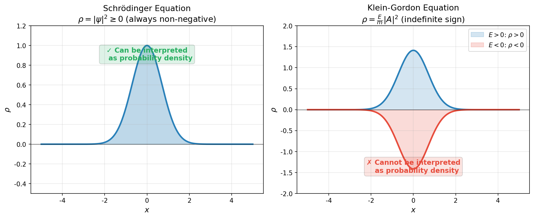
Fig. 1.1: The probability density problem of the Klein-Gordon equation. Left — For the Schrödinger equation, the probability density \(\rho = |\psi|^2 \geq 0\) is always non-negative. Right — For the Klein-Gordon equation, \(\rho = (E/m)|A|^2\), which can become \(\rho < 0\) for \(E < 0\) solutions.

🟡 Lina: Exactly. This is the fatal problem of the Klein-Gordon equation. The probability density can become negative, which means \(\rho\) cannot be interpreted as a probability density. I've summarized the contrast with the Schrödinger equation in Fig. 1.1 "The probability density problem of the Klein-Gordon equation. Left". The table below also compares the probability density properties of each equation.

Table 1.1: Comparison of probability densities in the Schrödinger and Klein-Gordon equations

	Schrödinger Equation	Klein-Gordon Equation
Order of time derivative	1st order	2nd order
Probability density \(\rho\)	$	\psi
Problem for \(E < 0\)	Negative energy solutions don't exist	\(\rho < 0\) → probability interpretation breaks down
Lorentz covariance	Not satisfied	Satisfied

🔵 Kai: So is the Klein-Gordon equation useless?

🟡 Lina: It can't be used as a single-particle wave function. But as we'll see later, when reinterpreted within the framework of quantum field theory, \(\rho\) takes on meaning not as a probability density but as a charge density. Negative \(\rho\) corresponds to negative charge — that is, antiparticles. But that's a story for later. For now, just remember that "within the framework of single-particle quantum mechanics, the Klein-Gordon equation breaks down."

✅ Comprehension Check: What is the fundamental reason why the "probability density" \(\rho\) of the Klein-Gordon equation can become negative?

Answer

Because the Klein-Gordon equation is second-order in time, the expression for \(\rho\) contains the time derivative \(\partial\phi/\partial t\). As a result, the sign of \(\rho\) depends on the sign of the energy \(E\), and for \(E < 0\) solutions, \(\rho < 0\). This contrasts with the Schrödinger equation (first-order in time), where \(\rho = |\psi|^2 \geq 0\) is automatically guaranteed.

📝 Exercises:

• Calculation of the Klein-Gordon probability density → Problem M-1. Lorentz Covariance of the Probability Current Density for the Klein-Gordon Equation

---

1.3　The Dirac Equation and Antiparticles — A Genius Idea to Return to First Order

🟡 Lina: Let's organize the problems with the Klein-Gordon equation — there were two:

1. The probability density can become negative — in Eq. (1.10), \(\rho < 0\) when \(E < 0\)
2. The physical interpretation of negative energy solutions is unclear — Eq. (1.9) admits \(E = -\sqrt{|\mathbf{p}|^2 + m^2}\), but what is "a particle with negative energy"?

Dirac attributed these problems to "the time derivative being second order" and attempted to construct a relativistic equation that is first-order in time.

🔵 Kai: But to maintain Lorentz covariance, time and space need to be treated on equal footing, right? If time is first-order, then space must also be first-order...

🟡 Lina: Sharp. That's precisely Dirac's genius insight. He sought an equation of the form:

\[ i\frac{\partial \psi}{\partial t} = \left(-i\boldsymbol{\alpha} \cdot \nabla + \beta m\right)\psi \tag{1.11} \]

Here \(\boldsymbol{\alpha} = (\alpha^1, \alpha^2, \alpha^3)\) and \(\beta\) are unknown objects. It turns out that if these are ordinary numbers (scalars), the relativistic dispersion relation \(E^2 = |\mathbf{p}|^2 + m^2\) cannot be reproduced.

⚪ Mei: A similar discussion came up in Quantum Mechanics Ch. 27.

🟡 Lina: Yes. We only stated the conclusion back then, but let's look at it more carefully now. I'll show that \(\boldsymbol{\alpha}\) and \(\beta\) cannot be ordinary numbers (scalars) if we want to reproduce the relativistic dispersion relation. Writing the right side of Eq. (1.11) as \(\hat{H} = \boldsymbol{\alpha} \cdot \mathbf{p} + \beta m\) (\(\mathbf{p} = -i\nabla\)), for energy eigenstates \(\hat{H}\psi = E\psi\) holds. Applying \(\hat{H}\) from the left once more gives \(\hat{H}^2\psi = \hat{H}(E\psi) = E(\hat{H}\psi) = E^2\psi\) (since \(E\) is just a number, it commutes with \(\hat{H}\)). So \(\hat{H}^2\psi = E^2\psi\) must hold, and to reproduce the dispersion relation \(E^2 = |\mathbf{p}|^2 + m^2\), we need \(\hat{H}^2\) to equal \((|\mathbf{p}|^2 + m^2)\,I\) (\(I\) is the identity matrix. Since \(\hat{H}\) is a matrix, the right side must also be a matrix for the equality to hold. The important point is that when \(\hat{H}^2\) acts on any plane wave \(e^{i\mathbf{p}\cdot\mathbf{x}}\), the result must be \((|\mathbf{p}|^2 + m^2)\,I\) times that plane wave — meaning as operators, \(\hat{H}^2 = (\hat{\mathbf{p}}^2 + m^2)\,I\) must hold. Below, we consider the action on plane waves and replace \(\hat{\mathbf{p}}\) with its eigenvalue \(\mathbf{p}\)). Let's compute \(\hat{H}^2\).

🔵 Kai: Squaring \(\hat{H}\) means multiplying \(\hat{H}\) by itself, right?

🟡 Lina: We square \(\hat{H} = \alpha^1 p_1 + \alpha^2 p_2 + \alpha^3 p_3 + \beta m\). With 4 terms it looks complicated at first, but let's build intuition with a simpler example. If there are only 2 terms, say \((A + B)^2\), then it's \(A^2 + AB + BA + B^2\) (note \(AB \neq BA\) for matrices). For 3 terms, \((A + B + C)^2 = A^2 + B^2 + C^2 + (AB + BA) + (AC + CA) + (BC + CB)\) — it separates into "squares of the same thing" and "products of different pairs (in both orders)." The 4-term case has the same structure, picking up products of all pairs. Organizing gives 4 types:

1. Products of the same thing: \(\alpha^1 p_1 \cdot \alpha^1 p_1 = (\alpha^1)^2 p_1^2\), etc. → \(\sum_i (\alpha^i)^2 p_i^2\)
2. Products of different \(\alpha\)'s: both \(\alpha^1 p_1 \cdot \alpha^2 p_2\) and \(\alpha^2 p_2 \cdot \alpha^1 p_1\) appear → \(\sum_{i<j}(\alpha^i \alpha^j + \alpha^j \alpha^i)p_i p_j\)
3. Products of \(\alpha\) and \(\beta\): \(\alpha^i p_i \cdot \beta m\) and \(\beta m \cdot \alpha^i p_i\) → \(\sum_i(\alpha^i \beta + \beta \alpha^i)m\,p_i\)
4. Product of \(\beta\) with itself: \(\beta m \cdot \beta m = \beta^2 m^2\)

Summarizing:

\[ \hat{H}^2 = \underbrace{\sum_i (\alpha^i)^2 p_i^2}_{\text{same-index terms}} + \underbrace{\sum_{i<j}(\alpha^i \alpha^j + \alpha^j \alpha^i)p_i p_j}_{i \neq j \text{ cross terms}} + \sum_i(\alpha^i \beta + \beta \alpha^i)m\,p_i + \beta^2 m^2 \]

Here \(\sum_{i<j}\) means "pick each pair of \(i\) and \(j\) exactly once without repetition" (for 3 dimensions: \((i,j) = (1,2), (1,3), (2,3)\), giving 3 terms). And \(\alpha^i \alpha^j + \alpha^j \alpha^i\) appears with products in both orders because \(\alpha^i\) are matrices, so \(\alpha^i \alpha^j \neq \alpha^j \alpha^i\) in general (the order of products cannot generally be swapped).

⚪ Mei: Because they're matrices, the order of products matters and \(AB + BA\) can't be simplified — this leads to anticommutation relations.

🟡 Lina: Let's see this concretely. When expanding \((A + B)^2\), taking \(A\) from the first \((A + B)\) and \(B\) from the second gives \(AB\). Taking \(B\) from the first and \(A\) from the second gives \(BA\). For ordinary numbers, \(AB = BA\) so \(AB + BA = 2AB\) can be combined, but for matrices this doesn't work, so \(AB + BA\) must be kept as is. The 4-term case is the same — there are 2 orderings for picking \(\alpha^i p_i\) and \(\alpha^j p_j\), giving \(\alpha^i \alpha^j p_i p_j + \alpha^j \alpha^i p_j p_i = (\alpha^i \alpha^j + \alpha^j \alpha^i)p_i p_j\).

🔵 Kai: Ah right, matrix multiplication changes the result when you swap the order. We saw examples where \(AB \neq BA\) when we used matrices in quantum mechanics. But can we swap \(\alpha^i\) and \(p_i\)? Is \(\alpha^i p_i\) the same as \(p_i \alpha^i\)?

🟡 Lina: Good check. \(\alpha^i\) are constant matrices that don't depend on space, and \(p_i = -i\partial/\partial x^i\) is a differential operator with respect to spatial coordinates. Differentiation acts on "the function to its right," but since \(\alpha^i\) is a constant, differentiating it gives nothing. So \(p_i \alpha^i = \alpha^i p_i\) and they can be freely interchanged (alternatively, as I mentioned, if we act on plane waves and replace \(p_i\) with its eigenvalue — just a number — then a number and a matrix trivially commute). On the other hand, \(\alpha^i\)'s are matrices so their order matters — \(\alpha^i \alpha^j \neq \alpha^j \alpha^i\) holds in general.

🟡 Lina: More specifically, from \(\sum_i \alpha^i p_i\), taking the \(i\)-th term \(\alpha^i p_i\) and the \(j\)-th term \(\alpha^j p_j\) (\(i \neq j\)) and multiplying gives \(\alpha^i p_i \cdot \alpha^j p_j\) and \(\alpha^j p_j \cdot \alpha^i p_i\) in two orderings. As we just confirmed, \(p_i\) and \(\alpha\) can be freely interchanged, so these become \(\alpha^i \alpha^j p_i p_j\) and \(\alpha^j \alpha^i p_i p_j\), and adding gives \((\alpha^i \alpha^j + \alpha^j \alpha^i) p_i p_j\).

For this to equal \(|\mathbf{p}|^2 + m^2\), we need:

• For \(\sum_i (\alpha^i)^2 p_i^2 = I\,|\mathbf{p}|^2\): \((\alpha^i)^2 = I\) (identity matrix. \(I \cdot |\mathbf{p}|^2\) means "multiply every component by \(|\mathbf{p}|^2\)")
• For the \(i \neq j\) cross terms \((\alpha^i \alpha^j + \alpha^j \alpha^i)p_i p_j\) to all vanish: \(\alpha^i \alpha^j + \alpha^j \alpha^i = 0\) (\(i \neq j\))
• For the \(\alpha\)-\(\beta\) cross terms \((\alpha^i \beta + \beta \alpha^i)m\,p_i\) to vanish: \(\alpha^i \beta + \beta \alpha^i = 0\) (this must hold for arbitrary momentum \(p_i\), so the coefficient matrix itself must be zero)
• For \(\beta^2 m^2 = m^2\): \(\beta^2 = I\)

🔵 Kai: "Setting the unwanted terms to zero" — collecting all those conditions gives anticommutation relations!

🟡 Lina: Writing them all together:

\[ \{\alpha^i, \alpha^j\} = 2\delta^{ij}I, \qquad \{\alpha^i, \beta\} = 0, \qquad \beta^2 = I \tag{1.12} \]

Here \(\{A, B\} \equiv AB + BA\) is the anticommutator, and \(I\) is the identity matrix (physics textbooks often omit \(I\) and write just \(1\), but don't forget that \(\alpha^i\) and \(\beta\) are matrices). The first condition combines \((\alpha^i)^2 = I\) when \(i = j\) and \(\alpha^i \alpha^j + \alpha^j \alpha^i = 0\) when \(i \neq j\) into a single equation. These conditions were also derived in Quantum Mechanics Ch. 27, but we've reconfirmed them here.

🔵 Kai: Anticommutation relations! The plus version of commutation relations \([A, B] = AB - BA\).

🟡 Lina: Exactly. And the smallest matrices satisfying these conditions are \(4 \times 4\). This means the wave function \(\psi\) is a 4-component column — a spinor. You might think "4 components, so it's the same as a 4-dimensional vector?" but it transforms differently under coordinate transformations than a 4-vector. That's why we distinguish it as a "spinor." We'll cover this in detail in Ch. 5; for now, just remember "the Dirac equation's wave function is a special object with 4 components."

🔵 Kai: What do the 4 components represent?

🟡 Lina: Of the 4 components, 2 correspond to spin-up and spin-down electrons, and the remaining 2 correspond to the antiparticle — the positron. I've summarized this correspondence in Fig. 1.2 "The 4-component structure of the Dirac spinor".

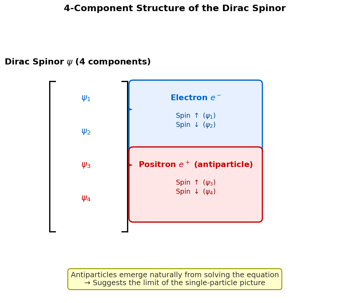
Fig. 1.2: The 4-component structure of the Dirac spinor. The upper 2 components (\(\psi_1, \psi_2\)) correspond to spin-up and spin-down electrons, while the lower 2 components (\(\psi_3, \psi_4\)) correspond to spin-up and spin-down positrons (antiparticles). Antiparticles emerge naturally just from solving the equation.

🔵 Kai: It's surprising that antiparticles come out just from solving the equation... but if 2 of the 4 components are antiparticles, isn't that the same as assuming "antiparticles exist" from the start? Or do they emerge without any such assumption? Also, what happened to the probability density problem?

🟡 Lina: Let me answer the first question. Dirac did not assume the existence of antiparticles. What he assumed was only "construct an equation that is first-order in time and space and Lorentz covariant." To satisfy this condition, at least 4 components are needed, and solving the equation yields negative energy solutions — interpreting these physically gives antiparticles. In other words, antiparticles are not an assumption but a consequence derived from the requirements of Lorentz covariance and quantum mechanics.

⚪ Mei: The only assumptions are "first-order and Lorentz covariant," and antiparticles are a consequence — beautiful.

🟡 Lina: And regarding the probability density problem. The Dirac equation partially resolved the Klein-Gordon equation's problems. The probability density \(\rho = \psi^\dagger \psi = |\psi_1|^2 + |\psi_2|^2 + |\psi_3|^2 + |\psi_4|^2 \geq 0\) is always non-negative.

🔵 Kai: Oh! So the Dirac equation has no problems?

🟡 Lina: The probability density problem is solved. But negative energy solutions still exist. Dirac interpreted these through the "Dirac sea" picture — all negative energy states are filled with fermions, and when a "hole" opens there, it's observed as a particle with positive energy and positive charge (the positron).

🔵 Kai: But wait. "Filling all negative energy states" requires infinitely many electrons, doesn't it? Do infinitely many particles really exist? And for particles like photons that can occupy the same state in any number, you can't "fill everything up" in the first place...

🟡 Lina: Sharp observations, both correct. The second one is particularly fatal. The Dirac sea picture only works for fermions — particles that obey the Pauli exclusion principle and can fill each state one at a time. For bosons, there is no exclusion principle, so "filling all states" is simply impossible. I've illustrated the Dirac sea picture in Fig. 1.3 "The Dirac sea picture. Left".

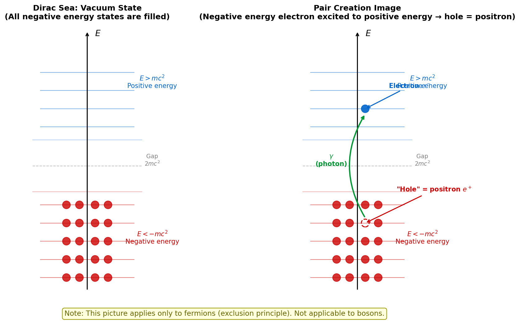
Fig. 1.3: The Dirac sea picture. Left — Vacuum state: all negative energy states are filled with fermions. Right — Pair creation: when a photon's energy excites a negative-energy electron to positive energy, the remaining "hole" is observed as a positron. This picture is applicable only to fermions (which obey the exclusion principle).

🔵 Kai: Wait, so how do we deal with negative energy solutions for bosons? If the Dirac sea can't be used, how do we interpret them?

🟡 Lina: Exactly. In the end, to fundamentally resolve the problem of negative energy solutions, we must go beyond the framework of single-particle wave functions altogether. That's quantum field theory. Let me organize the discussion so far.

Table 1.2: Problems of single-particle relativistic equations and resolution by quantum field theory

	Klein-Gordon Equation	Dirac Equation	Quantum Field Theory (QFT)
Time derivative	2nd order	1st order	— (quantize the field)
Probability density \(\rho \geq 0\)	× Breaks down	○ Resolved	○ Resolved
Negative energy solutions	Exist	Exist (interpreted via Dirac sea)	Naturally interpreted as antiparticles
Change in particle number	Cannot describe	Cannot describe	○ Naturally described
Applicability to bosons	Yes (with problems)	No (fermions only)	○ Applicable to all particles

✅ Comprehension Check: Explain why the Dirac equation can solve the Klein-Gordon equation's "negative probability density" problem, from the perspective of the order of derivatives.

Answer

Because the Dirac equation is first-order in time, the probability density takes the form \(\rho = \psi^\dagger \psi\) (sum of absolute values squared of each component), guaranteeing \(\rho \geq 0\) at all times. The Klein-Gordon equation, being second-order in time, has time derivatives appearing in \(\rho\), making its sign indefinite.

---

1.4　Why Particle Creation and Annihilation Are Inevitable

🟡 Lina: So far we've seen that "relativistic equations as single-particle wave functions face difficulties." Next, let's understand from a more physical perspective that "phenomena where particle number changes are unavoidable." I'll present 3 arguments, and then also examine the requirement from causality. I've shown the overall picture in advance in Fig. 1.4 "3+1 arguments for why particle creation and annihilation are inevitable".

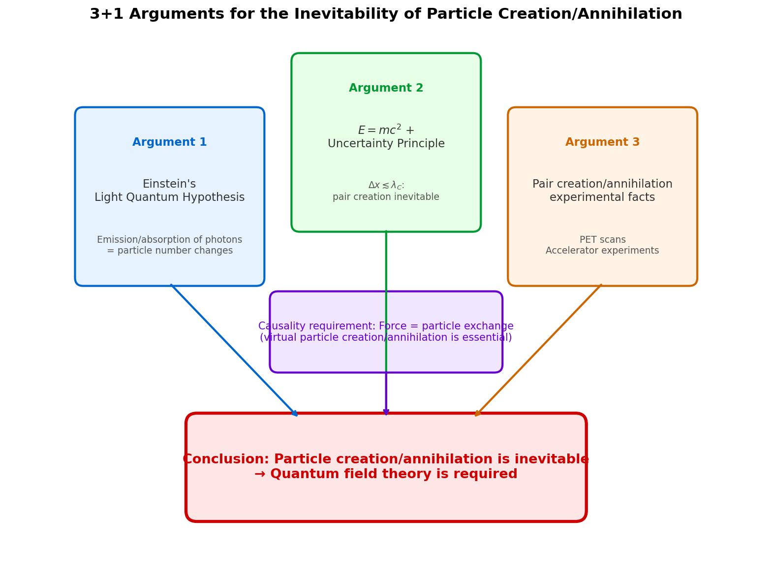
Fig. 1.4: 3+1 arguments for why particle creation and annihilation are inevitable. Three independent physical arguments (photon hypothesis, \(E=mc^2\) with the uncertainty principle, experimental fact of pair creation) plus the requirement of causality all point to the conclusion that "quantum field theory is needed."

Argument 1: Einstein's Photon Hypothesis — Photons Are Born and Die

🟡 Lina: Historically, particle creation and annihilation were first recognized for photons.

In 1900, Planck proposed the hypothesis that electromagnetic energy is not continuous but discrete to explain the blackbody radiation spectrum (I'll write \(\hbar\) explicitly here):

\[ E_n = n\hbar\omega \qquad (n = 0, 1, 2, \ldots) \tag{1.13} \]

🔵 Kai: This means electromagnetic waves of frequency \(\omega\) can only have energies in integer multiples of \(\hbar\omega\), right?

🟡 Lina: Yes. And in 1905, Einstein pushed this further and proposed that light itself is a collection of particles — photons — each carrying energy \(\hbar\omega\) and momentum \(\hbar\mathbf{k}\). This is the photon hypothesis.

🟡 Lina: There are several decisive experimental evidences that this hypothesis is correct:

1. Photoelectric effect: If the frequency of light is below a certain threshold, no electrons are ejected no matter how intense the light is. This is naturally explained if light collides as particles with energy \(E = \hbar\omega\).

2. Compton scattering: When X-rays are scattered by electrons, the wavelength changes depending on the scattering angle (Fig. 1.5 "Conceptual diagram of Compton scattering"). The scattered photon gives up some of its energy to the electron, so its wavelength becomes longer. This is explained by thinking of the photon as a particle with momentum \(\mathbf{p} = \hbar\mathbf{k}\) that collides with the electron, exchanging energy and momentum.

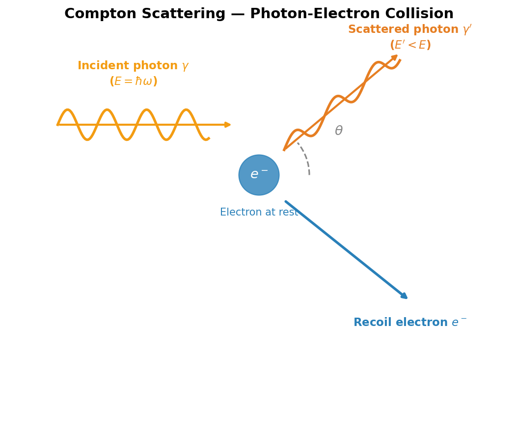
Fig. 1.5: Conceptual diagram of Compton scattering. An incident photon \(\gamma\) collides with a stationary electron \(e^-\), producing a scattered photon \(\gamma'\) at angle \(\theta\) and a recoil electron. The scattered photon loses energy and its wavelength increases.

🔵 Kai: In Compton scattering, a photon hits an electron and bounces off, right? But is that a story about "the number of photons changing"?

🟡 Lina: Good question. Compton scattering itself is a process where 1 photon goes in and 1 comes out, so the photon number doesn't change. But think about it. When an atom emits light, a photon is born. When an atom absorbs light, a photon dies. This means the number of photons is not a conserved quantity — creation and annihilation happen routinely.

⚪ Mei: I see, photon number changing isn't a special situation — it happens in the ordinary process of atoms emitting and absorbing light.

🟡 Lina: Exactly. And since photons have zero mass, they can be created in any number as long as there's enough energy. "Quantum mechanics with a fixed number of particles" cannot describe such processes.

Argument 2: The Interplay of \(E = mc^2\) and the Uncertainty Principle — Pair Creation

🟡 Lina: The second argument makes the discussion from Quantum Mechanics Ch. 27 a bit more quantitative.

Einstein's mass-energy equivalence:

\[ E = mc^2 \tag{1.14} \]

This means "if energy \(E \geq 2mc^2\) is available, a particle-antiparticle pair of mass \(m\) can be created."

On the other hand, the energy-time uncertainty relation of quantum mechanics:

\[ \Delta E \cdot \Delta t \gtrsim \hbar \tag{1.15} \]

🔵 Kai: During a short time \(\Delta t\), a large energy fluctuation \(\Delta E\) is allowed — that's the idea, right? But is this the same kind of relation as \(\Delta x \cdot \Delta p \geq \hbar/2\)?

🟡 Lina: Strictly speaking, they have slightly different character. The \(\Delta x \cdot \Delta p\) version is rigorously derived from the commutation relation of operators, but for the energy-time version, "time is not an operator" so the same derivation doesn't work. However, here we're using it as an order-of-magnitude estimate — a calculation that only tracks the scale — so we write \(\sim\) or \(\gtrsim\) to mean "roughly this much." It's sufficient for quantitative arguments.

⚪ Mei: Not mathematically rigorous, but usable as a scale estimate — a common technique in physics.

🟡 Lina: Right. What can we conclude by combining these two?

🔵 Kai: What does the actual calculation look like?

🟡 Lina: Good question. Here I'll write \(\hbar\) and \(c\) explicitly (since we want specific numbers). If we try to localize a particle within a distance scale \(\Delta x\), the uncertainty principle gives a momentum fluctuation \(\Delta p \gtrsim \hbar / \Delta x\). Looking at the relativistic energy relation \(E = \sqrt{p^2c^2 + m^2c^4}\), when \(c\,\Delta p \gg mc^2\) (i.e., when the energy from momentum is much larger than the rest energy), we can approximate \(\sqrt{p^2c^2 + m^2c^4} \approx \sqrt{p^2c^2} = pc\) (since \(m^2c^4\) is negligibly small compared to \(p^2c^2\)). Under this approximation \(E \approx pc\), so the energy fluctuation from a momentum fluctuation \(\Delta p\) is simply \(\Delta E \approx c\,\Delta p\). This is exactly the same logic as "if \(x\) changes by \(\Delta x\) in a linear function \(y = cx\), then \(y\) changes by \(c\,\Delta x\)."

Let me check when this approximation is valid. Substituting \(\Delta p \sim \hbar/\Delta x\) into \(c\,\Delta p \gg mc^2\) gives \(\hbar c/\Delta x \gg mc^2\), i.e., \(\Delta x \ll \hbar/(mc) = \lambda_C\). So this approximation holds at distance scales shorter than the Compton wavelength — precisely the regime where pair creation becomes relevant. Therefore:

\[ \Delta E \sim c\,\Delta p \sim \frac{\hbar c}{\Delta x} \tag{1.16} \]

🔵 Kai: Oh, the smaller the distance, the larger the energy fluctuation!

🟡 Lina: When this energy fluctuation exceeds the rest energy of a particle-antiparticle pair, \(2mc^2\):

\[ \frac{\hbar c}{\Delta x} \gtrsim 2mc^2 \]

\[ \Delta x \lesssim \frac{\hbar}{2mc} = \frac{\lambda_C}{2} \tag{1.17} \]

Here \(\lambda_C = \hbar/(mc)\) is the particle's Compton wavelength. This means pair creation cannot be ignored at distance scales of order the Compton wavelength or smaller.

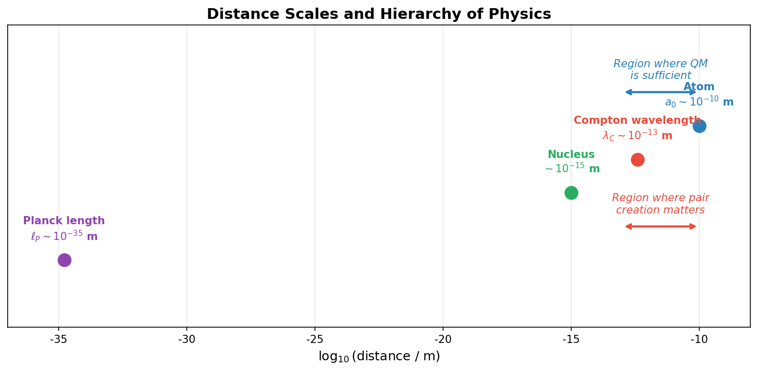
Fig. 1.6: Distance scales and the hierarchy of physics. At distances shorter than the Compton wavelength \(\lambda_C \sim 10^{-13}\) m, pair creation becomes important and single-particle quantum mechanics is insufficient.

⚪ Mei: Eq. (1.17) shows \(\lambda_C/2\) as the boundary. Trying to observe particles at shorter distances than this, pair creation can no longer be ignored.

🟡 Lina: Exactly. I've summarized the distance scales and hierarchy of physics in Fig. 1.6 "Distance scales and the hierarchy of physics". For electrons, \(\lambda_C \approx 3.86 \times 10^{-13}\) m, which is much smaller than atomic sizes (\(\sim 10^{-10}\) m). That's why atomic physics could ignore particle creation and annihilation. But at the scales dealt with in particle physics, they cannot be ignored.

🔵 Kai: I see... So even when trying to study "a single electron," at sufficiently fine scales, there's a possibility of electron-positron pairs popping into existence? But then, doesn't that mean "the electron's mass" and "the electron's charge" are values that include the effects of these surrounding virtual pairs?

🟡 Lina: Sharp intuition. That's actually exactly right — the observed mass and charge are "dressed values" that include the effects of virtual pairs. We'll address this head-on in Part V on renormalization. Physicist Victor Weisskopf also emphasized this point — "In relativistic quantum mechanics, a single-particle theory does not exist."

📝 Exercises:

• Compton wavelength and the uncertainty principle → Problem B-5. Calculation of the Compton Wavelength, Problem M-3. Compton Wavelength and Position Localization

Argument 3: The Experimental Fact of Pair Creation and Annihilation

🟡 Lina: The third argument is more directly experimental.

Pair annihilation: When an electron and positron meet, they mutually annihilate and become photons:

\[ e^- + e^+ \to \gamma + \gamma \tag{1.18} \]

Pair creation: When a photon with sufficient energy passes near an atomic nucleus, an electron-positron pair is born:

\[ \gamma \to e^- + e^+ \quad (\text{near an atomic nucleus}) \tag{1.19} \]

🔵 Kai: Has this actually been observed?

🟡 Lina: Of course. Pair annihilation is the very principle behind PET (Positron Emission Tomography) — a medical imaging technology. A radioactive substance that emits positrons is injected into the body, and when the positrons annihilate with electrons inside the body, the two resulting gamma rays are detected to create an image.

⚪ Mei: A routinely used medical technology is evidence of particle creation and annihilation.

🟡 Lina: Yes. Particle creation and annihilation is not "a rare phenomenon that only occurs in extreme situations" — it's a fundamental property of nature. A theory that cannot describe this is fundamentally incomplete. I've summarized the processes of pair creation and annihilation in Fig. 1.7 "Processes of pair creation and annihilation. Left".

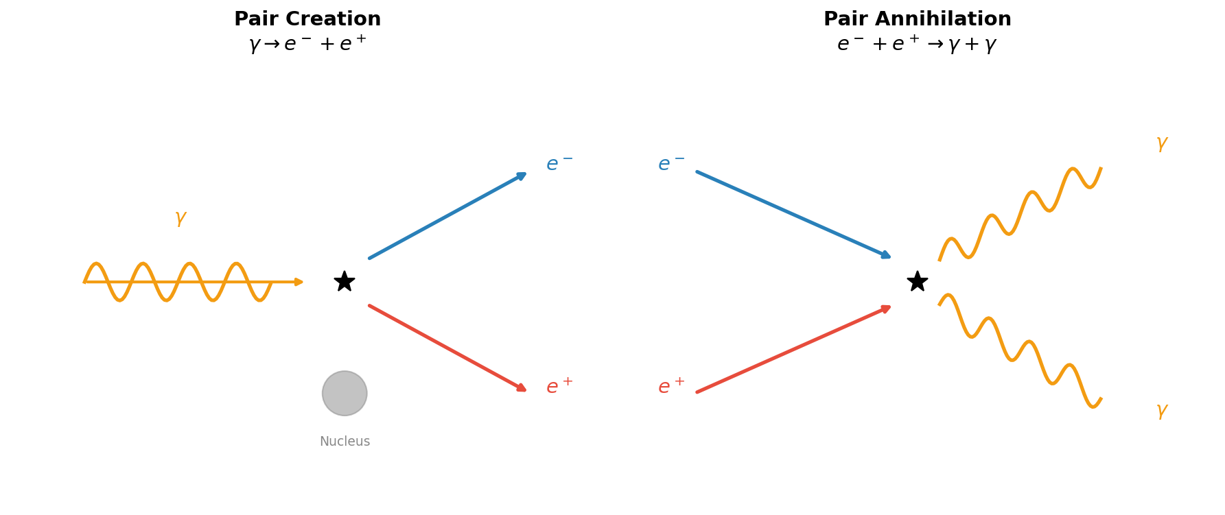
Fig. 1.7: Processes of pair creation and annihilation. Left — Pair creation: a high-energy photon \(\gamma\) is converted into an electron \(e^-\) and positron \(e^+\) pair near an atomic nucleus. Right — Pair annihilation: an electron and positron meet, annihilate, and emit 2 gamma rays. PET scans are medical technology utilizing this pair annihilation.

✅ Comprehension Check: Calculate the electron's Compton wavelength \(\lambda_C = \hbar/(m_e c)\) and compare it with the size of an atom (Bohr radius \(a_0 \approx 0.53 \times 10^{-10}\) m).

Answer

\(\lambda_C = \frac{\hbar}{m_e c} = \frac{1.055 \times 10^{-34}}{9.11 \times 10^{-31} \times 3 \times 10^8} \approx 3.86 \times 10^{-13}\) m. Comparing with the Bohr radius \(a_0 \approx 5.3 \times 10^{-11}\) m gives \(\lambda_C / a_0 \approx 7 \times 10^{-3}\), meaning the Compton wavelength is about 1/140 of the atomic size. Pair creation can be ignored at atomic scales but not at nuclear or particle physics scales.

📝 Exercises:

• Threshold energy for pair creation → Problem B-7. Time Scale of Pair Creation from the Uncertainty Relation

---

1.5　The Requirement of Causality — Forces Are Transmitted by Particle Exchange

🟡 Lina: There's another important reason why particle creation and annihilation are necessary. It's to preserve causality — the fundamental principle of relativity that "information cannot travel faster than light."

🔵 Kai: How are causality and particle creation/annihilation related?

🟡 Lina: Recall Coulomb's law. When two charges \(q_1\), \(q_2\) are separated by distance \(r\), the force between them is (here I'll write it in the familiar SI units. The choice of unit system isn't essential — what matters is the structure of the equation):

\[ F = \frac{q_1 q_2}{4\pi\varepsilon_0 r^2} \]

Look at this equation carefully. The force \(F\) is determined only by "the distance \(r\) right now," with no time delay built in. This means if one charge is moved and \(r\) changes, the other instantaneously feels the new force — no matter how far apart they are. This implies "information travels faster than light," violating causality.

🔵 Kai: Ah, isn't this the same problem as Newton's law of universal gravitation? That one also implicitly assumed "gravity propagates instantaneously," right?

🟡 Lina: Exactly. Newton's law of gravitation also had the same problem of "the force between two masses is determined only by distance and propagates instantaneously" (we discussed this in detail in General Relativity Ch. 1). The electromagnetic force has exactly the same issue. In classical electromagnetism, this problem was solved by introducing "electromagnetic fields." Forces propagate through fields at the speed of light. So what happens in quantum theory?

🔵 Kai: The quantum theory also solves it with "fields"?

🟡 Lina: In quantum field theory, forces are interpreted as being transmitted by virtual particle exchange. What classical electromagnetism describes as "the electromagnetic field transmitting force at the speed of light" becomes "virtual photon exchange" in the language of quantum theory. The electromagnetic force between two electrons repelling each other is described as a process where one electron emits a virtual photon and the other absorbs it. Since photons travel at the speed of light, causality is preserved.

🔵 Kai: "Exchanging virtual photons produces a force" — what's the image? Like throwing balls back and forth causes repulsion?

🟡 Lina: Yes, the ball-tossing analogy works nicely. If two people standing on ice throw a ball back and forth, the thrower recoils backward and the catcher is pushed — as a result, they move apart. This is the image for "repulsion." However, for attractive forces this classical analogy doesn't quite work, and quantum mechanical effects become essential. The precise argument will be given in Ch. 8 with Feynman diagrams.

🔵 Kai: I see. So a "virtual photon" is a photon whose existence is permitted for a short time by the uncertainty principle?

🟡 Lina: Intuitively, yes. The uncertainty relation \(\Delta E \cdot \Delta t \gtrsim \hbar\) permits "borrowing" energy for a short time. During that time, a photon is born, reaches the other particle, and disappears — this process is the true nature of force. However, one caveat: virtual particles, unlike ordinary particles, do not satisfy \(E^2 = p^2c^2 + m^2c^4\). This relation is "the condition that holds when a particle of mass \(m\) travels freely" and is separate from energy conservation itself. You might think "Wait, doesn't that violate energy conservation?" but the overall process — from the photon being created to being absorbed by the other particle — does properly conserve energy and momentum. The virtual particle can deviate from \(E^2 = p^2c^2 + m^2c^4\) only for the short time permitted by the uncertainty principle. In the end, the books balance. So virtual particles cannot be directly caught by a detector — they're "backstage actors" that mediate forces. The precise definition will be given in Ch. 8 with Feynman diagrams; for now, think of them as "particles that aren't directly observed but mediate forces, deviating from the usual energy-momentum relation."

⚪ Mei: They don't satisfy the energy-momentum relation, yet overall conservation laws hold — strange, but the uncertainty principle permits it.

🟡 Lina: To summarize the discussion so far: to transmit forces while preserving causality, the creation and annihilation of mediating particles is essential. Not just for the electromagnetic force — all fundamental forces are transmitted by this mechanism. The table below summarizes which force is mediated by which particle. See Fig. 1.8 "Electromagnetic force via virtual photon exchange" for the virtual photon exchange picture, and Fig. 1.9 "The four fundamental forces and their mediating particles" for the overall picture of the four forces.

⚪ Mei: Causality also leads to the same conclusion. The photon hypothesis, \(E=mc^2\) with the uncertainty principle, the experimental fact of pair creation, plus the requirement of causality — four independent arguments all point to "we need a theory that can handle particle creation and annihilation."

Table 1.3: Correspondence between fundamental forces and mediating particles

Force	Mediating Particle
Electromagnetic force	Photon \(\gamma\)
Weak force	\(W^\pm\), \(Z^0\) bosons
Strong force	Gluons
Gravity	Graviton (undetected)

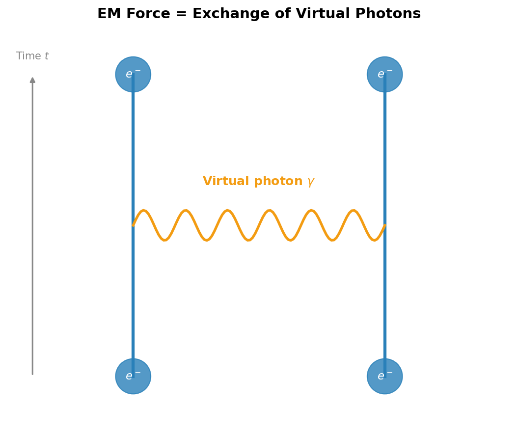
Fig. 1.8: Electromagnetic force via virtual photon exchange. The electromagnetic force between two electrons is described as virtual photon \(\gamma\) exchange. Since photons travel at the speed of light, causality is preserved.

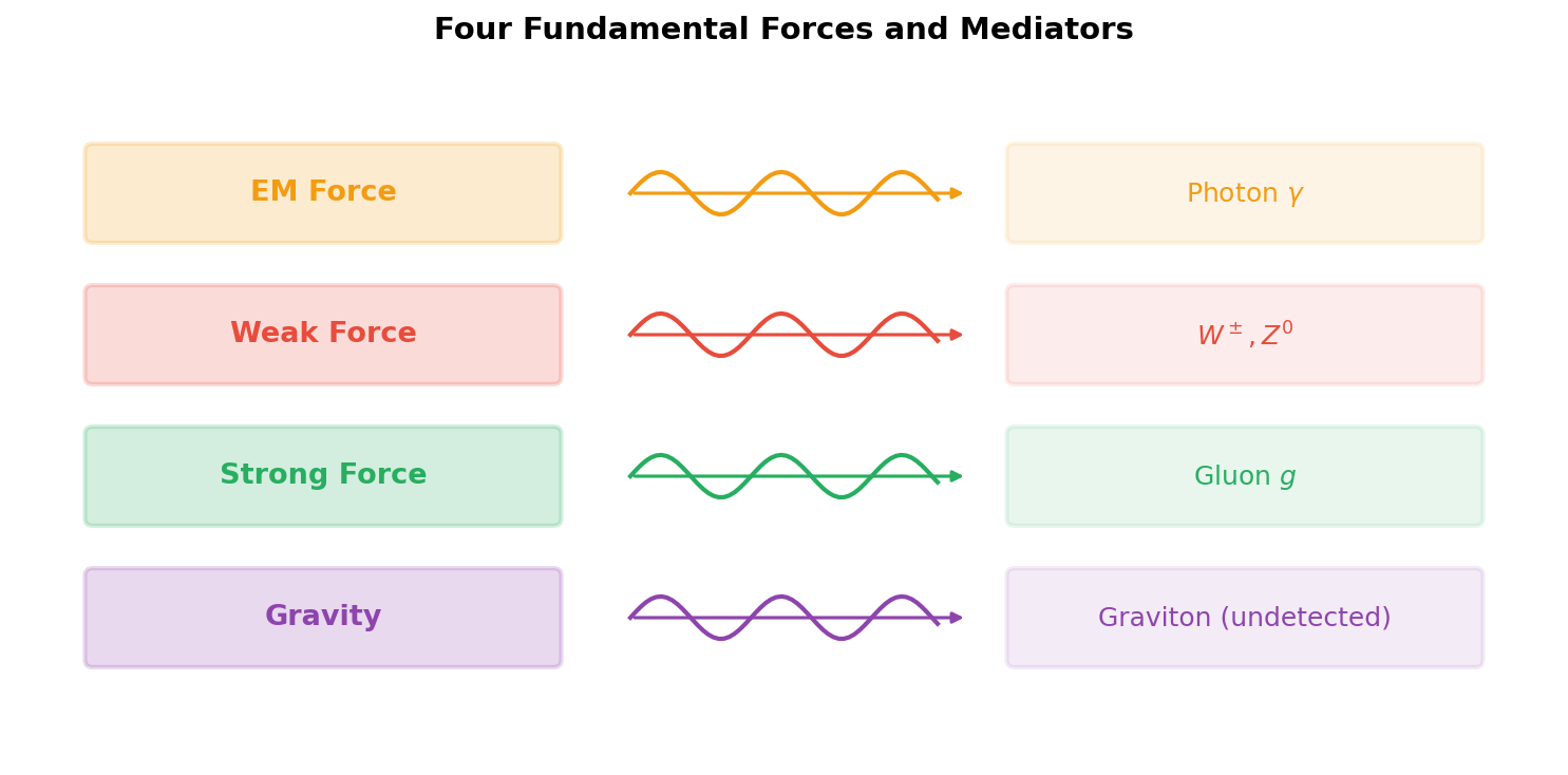
Fig. 1.9: The four fundamental forces and their mediating particles. The four fundamental forces of nature and the particles that mediate each one. The graviton has not yet been directly detected.

🔵 Kai: Wow... If the true nature of forces is "particle exchange," then a theory that can't handle particle creation and annihilation can't even describe forces! But the fact that the graviton hasn't been found — does that mean gravity might work by a different mechanism?

🟡 Lina: Sharp question. Currently the graviton is undetected, but theoretically gravity is expected to be described by the same mechanism — graviton exchange. However, there are mountains of unsolved problems in quantizing gravity, which is a topic for Ch. 24. This is the argument from causality that "particle creation and annihilation are inevitable." To transmit forces while respecting relativistic causality, creation and annihilation of mediating particles is essential.

🔵 Kai: If all four forces are transmitted by the same mechanism, particle creation and annihilation really can't be avoided.

---

1.6　A Shift in Perspective — "Particles Are Vibrational Modes of Fields"

🟡 Lina: Summarizing the discussion so far: "quantum mechanics with a fixed number of particles" cannot describe the relativistic world. So what should we do? This is where a fundamental shift in perspective is needed.

Asymmetry in Classical Physics

🟡 Lina: First, let me point out the asymmetry in how "particles" and "fields" are treated in classical physics.

Table 1.4: Asymmetry between matter particles and light in classical physics

	Matter particles (electrons, etc.)	Light
Classical status	Assumed from the start as fundamental constituents of nature	Described as waves of the electromagnetic field
Description	Newtonian mechanics (point particle mechanics)	Maxwell's equations (field theory)

🔵 Kai: Electrons are "particles that are just there from the beginning" while photons emerge as "oscillations of the electromagnetic field"... that is indeed asymmetric.

🟡 Lina: But in quantum mechanics, both electrons and photons exhibit wave-particle duality. In the double-slit experiment, electrons produce interference patterns; in the photoelectric effect, light behaves as particles.

🔵 Kai: If electrons and photons are on equal footing... and photons are "oscillations of the electromagnetic field"... then is there some kind of "field" for electrons too, whose oscillations are electrons? But I've never heard of an "electron field"...

🟡 Lina: Kai, great intuition. That's precisely the core of quantum field theory. The "electron field" is invisible but truly exists — just as excitations of the electromagnetic field are photons, excitations of the "electron field" are electrons. The idea is to treat all particles uniformly as excitations of fields.

The Worldview of Quantum Field Theory

🟡 Lina: The worldview of quantum field theory can be stated in one sentence:

All particles in the universe are excitations of quantum fields defined throughout all of space and time.

Specifically:

• Photon = quantized excitation of the electromagnetic field \(A_\mu\)
• Electron = quantized excitation of the Dirac field \(\psi\)
• Higgs particle = quantized excitation of the Higgs field \(\phi\)

Table 1.5: Main particles of the Standard Model and their corresponding fields

Particle	Corresponding Field	Spin	Field Type
Photon \(\gamma\)	Electromagnetic field \(A_\mu\)	1	Vector field (gauge field)
Electron \(e^-\)	Dirac field \(\psi_e\)	1/2	Spinor field
Quark \(q\)	Dirac field \(\psi_q\)	1/2	Spinor field
Higgs particle \(H\)	Scalar field \(\phi\)	0	Scalar field
Gluon \(g\)	Yang-Mills field \(A_\mu^a\)	1	Vector field (gauge field)
Graviton	Metric tensor field \(g_{\mu\nu}\)	2	Tensor field

🟡 Lina: You see names like "gauge field," "Yang-Mills field," and "spinor field" in the table that you haven't encountered before, but for now just grasp that "there's a corresponding field for each type of particle." We'll learn the detailed meaning of each from Part II onward. As an analogy, the entire surface of a pond is the "field," and the ripples that appear on it are "particles."

🔵 Kai: Ah, I get it! Ripples appear and disappear, so particle creation and annihilation correspond to "vibrations of the field starting and stopping"!

🟡 Lina: Exactly. That's why changes in particle number can be naturally described.

⚪ Mei: So in quantum mechanics, the starting point was "particles exist," but in quantum field theory, the starting point is "fields exist" and particles emerge as a consequence — the protagonist changes.

🟡 Lina: Nicely summarized. Furthermore, this picture has another great benefit. All particles born from the same field have identical properties. The reason every electron has exactly the same mass, charge, and spin is that they're excitations of the same "electron field." Bolts made in a factory show slight differences under a microscope, but electrons are perfectly identical — this is a natural consequence of the QFT worldview that "ripples born from the same field have the same properties." I've illustrated this worldview in Fig. 1.10 "The worldview of quantum field theory. Left".

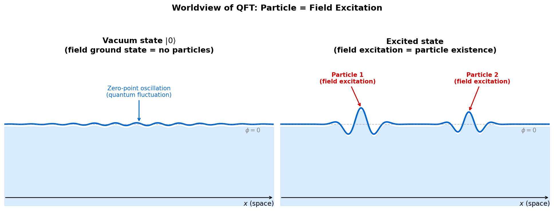
Fig. 1.10: The worldview of quantum field theory. Left — In the vacuum state, the field has only zero-point oscillations (quantum fluctuations). Right — When the field is locally excited, it is observed as a "particle." The image is like ripples on the surface of a pond corresponding to particles.

⚪ Mei: So two things emerge simultaneously from the QFT worldview: the ability to naturally describe particle creation and annihilation, and the explanation of why identical particles are perfectly identical.

✅ Comprehension Check: Explain in 1–2 sentences why "all electrons are perfectly identical" from the perspective of quantum field theory.

Answer

All electrons are quantized excitations of the same "electron field," so properties such as mass, charge, and spin are perfectly identical. Even though the ripples are at different locations, as long as they are vibrations of the same surface (field), they inherently have the same properties.

---

1.7　Second Quantization and Fock Space

First Quantization and Second Quantization

🟡 Lina: Let me organize the history of quantization here. The development of quantum mechanics has two stages.

First quantization:

Particles behave like waves.

Classical mechanical variables (position \(x\), momentum \(p\)) are promoted to operators and the commutation relation \([\hat{x}, \hat{p}] = i\hbar\) is imposed. This is what we learned in the previous volume on quantum mechanics.

Second quantization:

Fields are promoted to operators, and the vibrational modes of the field come to behave as "particles."

Historically, this is sometimes expressed as "waves behave like particles" — when a classical wave (field) is quantized, its energy appears as discrete "particles." But what's actually being done is promoting fields to operators — this enables the description of phenomena where particle number changes.

🔵 Kai: "Making fields into operators"... concretely, what does that mean? Does something like a wave function become an operator?

🟡 Lina: Historically, it's sometimes put that way. "First, turning particles into waves (wave functions) was first quantization. Then quantizing those waves is second quantization" — that's where the name comes from. But be careful as this phrasing is misleading. In practice, we're not "quantizing the wave function again." From the modern perspective, the essence is promoting a classical field — a quantity like the electromagnetic field that has a value at each point in space — to a quantum operator. Both "first" and "second" are the same procedure — promoting classical mechanical variables to operators — the only difference is that the object of quantization changes from "particle position" to "field amplitude." So in modern usage, rather than insisting on the name "second quantization," it's more accurate to simply call it "field quantization."

⚪ Mei: The name has "second" only due to historical circumstances — the operation itself is the same.

🟡 Lina: What we're essentially doing is the same as first quantization — promoting classical mechanical variables to operators and imposing commutation relations. The only difference is that the "mechanical variable" is the field rather than the particle's position. "Promoting to operators" means the same procedure as turning \(x\) into \(\hat{x}\) in quantum mechanics — transforming a quantity that classically has a definite value into a quantum object whose value is indeterminate until measured. For fields, "the field amplitude at each point" becomes a quantum object that fluctuates.

⚪ Mei: So the same procedure that turned \(x\) into \(\hat{x}\) now turns \(\phi(\mathbf{x})\) into \(\hat{\phi}(\mathbf{x})\).

🟡 Lina: Exactly. The correspondence is summarized as follows (see also Fig. 1.11 "Second quantization and Fock space"). You'll see symbols like \(\hat{\pi}\) and \(\delta^3\) in the table that are new to you, but I'll explain each one right after the table, so for now just look at the correspondence structure as "the field version of what we did in quantum mechanics."

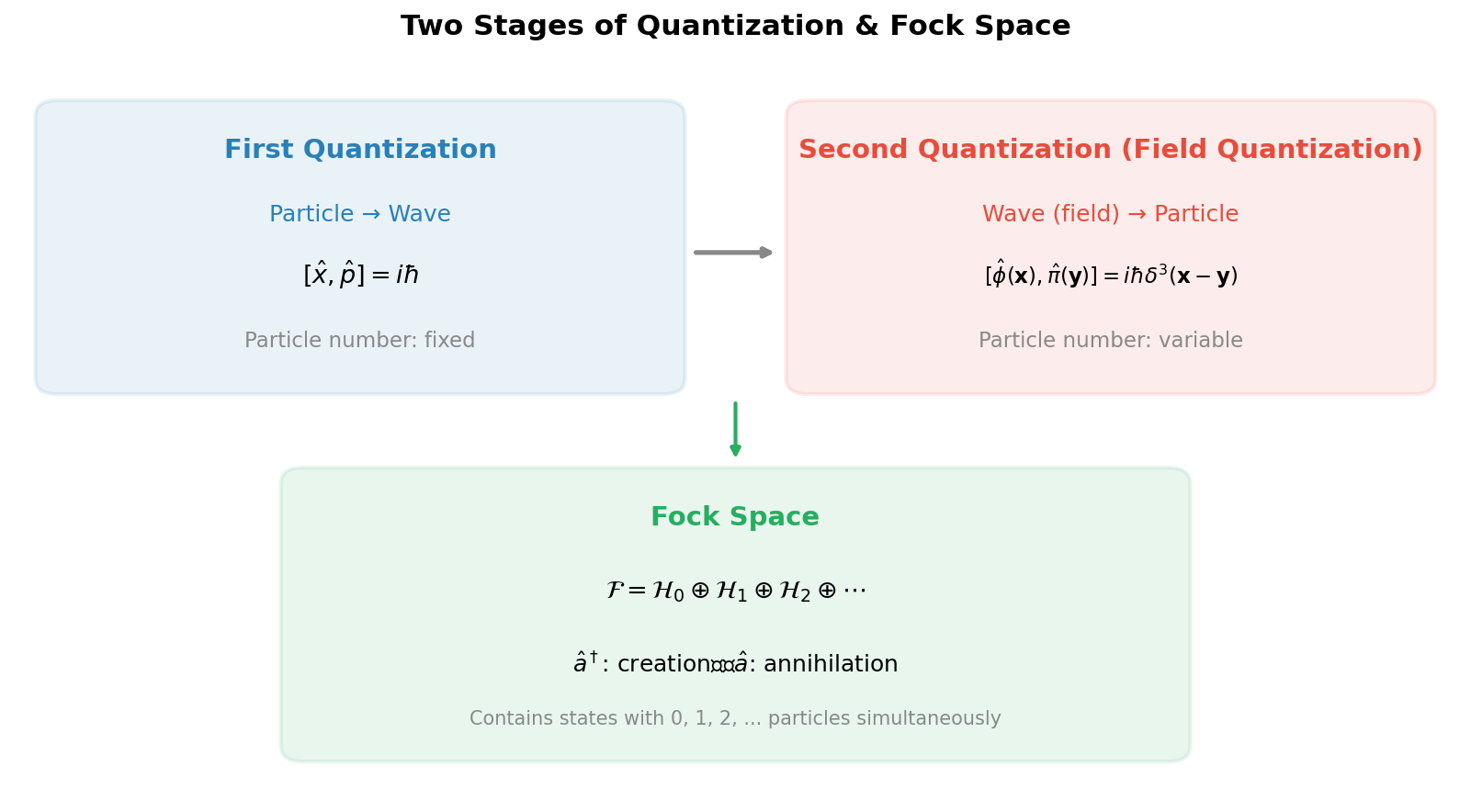
Fig. 1.11: Second quantization and Fock space. Comparison of first quantization (particle → wave) and second quantization (wave → particle). In second quantization, fields are promoted to operators and physics is described in Fock space where particle number is variable.

Table 1.6: Correspondence between first and second quantization

	Quantum Mechanics (First Quantization)	Quantum Field Theory (Second Quantization)
Dynamical variables	Particle position \(\hat{x}\), momentum \(\hat{p}\)	Field \(\hat{\phi}(\mathbf{x})\), conjugate momentum \(\hat{\pi}(\mathbf{x})\)
Commutation relation	\([\hat{x}, \hat{p}] = i\hbar\)	\([\hat{\phi}(\mathbf{x}, t), \hat{\pi}(\mathbf{y}, t)] = i\hbar\,\delta^3(\mathbf{x} - \mathbf{y})\) (equal time)
Role of \(\mathbf{x}\)	Dynamical variable representing where the particle is	Label (parameter) indicating which point in space

🔵 Kai: What's the "conjugate momentum" \(\hat{\pi}(\mathbf{x})\)? And I've never seen the symbol \(\delta^3\) before. Also, the "equal time" note is bothering me...

🟡 Lina: Three questions at once! Let me answer them in the order Kai raised them. First, the conjugate momentum \(\pi(\mathbf{x})\). Just as the particle's position \(x\) has a partner variable — the momentum \(p\) — the field \(\phi(\mathbf{x})\) also has a "partner variable." That's the conjugate momentum \(\pi(\mathbf{x})\). Roughly speaking, it represents "the vigor of the field's time variation," just as the particle's momentum \(p = m\dot{x}\) represents "the vigor of the position's time variation." More specifically, \(p = m\dot{x}\) represents "how fast the position \(x\) is changing." Similarly, \(\pi(\mathbf{x})\) represents "how fast the field value \(\phi(\mathbf{x})\) at point \(\mathbf{x}\) is changing in time." The precise definition will be introduced in Ch. 3 with the Lagrangian; for now, just hold onto this image.

🔵 Kai: I see, if \(p\) is "the rate of change of position," then \(\pi\) is "the rate of change of the field" — the correspondence is clean.

🟡 Lina: Next, \(\delta^3(\mathbf{x} - \mathbf{y})\). This is the 3-dimensional Dirac delta function, which has a value only when \(\mathbf{x} = \mathbf{y}\) and is zero otherwise. Think of it as the continuous version of the Kronecker delta \(\delta_{ij}\) (which equals 1 when \(i = j\) and 0 otherwise) used for discrete indices.

🔵 Kai: "Has a value" — what does that mean concretely? A function that has a value at only one point...

🟡 Lina: Intuitively, it's a special function that "has an infinitely sharp peak at \(\mathbf{x} = \mathbf{y}\) and is completely zero elsewhere, but the area (integral) of the peak is exactly 1." Its key property is \(\int \delta^3(\mathbf{x} - \mathbf{y})\, f(\mathbf{y})\, d^3y = f(\mathbf{x})\) — it "picks out the value of \(f\) at \(\mathbf{x}\)." For now, just remember the property "non-zero only at the same point \(\mathbf{x} = \mathbf{y}\)." The \(\delta^3\) appearing in the commutation relation expresses "fields at different points are independent."

Finally, the "equal time" condition — in quantum mechanics when we wrote \([\hat{x}, \hat{p}] = i\hbar\), \(\hat{x}\) and \(\hat{p}\) were quantities at the same time, right? The same applies in QFT: the commutation relation is defined as "the relationship between \(\hat{\phi}\) and \(\hat{\pi}\) at the same time \(t\)." The relationship between fields at different times is determined by the equations of motion (time evolution), which is a separate matter from the commutation relation. For now, just remember "the commutation relation establishes the fundamental relationship between fields at the same time."

🟡 Lina: Now look at the last row of the table. The role of \(\mathbf{x}\) changes fundamentally.

🔵 Kai: Ah, looking at the last row of the table, the role of \(\mathbf{x}\) changes. It was a dynamical variable in quantum mechanics, but becomes a label in quantum field theory... What does that mean? But in quantum mechanics, didn't we also use \(x\) in the wave function \(\psi(x)\) like a label?

🟡 Lina: Good catch. Indeed, when writing \(\psi(x)\) in the position representation, \(x\) looks like a label specifying "the probability amplitude at which position." But looking at the essential structure of quantum mechanics, \(\hat{x}\) exists as an operator, and \(\psi(x)\) is the projection onto the eigenstate \(|x\rangle\): \(\langle x|\psi\rangle\). In other words, \(x\) was a dynamical variable corresponding to the physical question "where is the particle?" — the object promoted to an operator. In contrast, in quantum field theory, \(\mathbf{x}\) is merely a parameter specifying "which point's field value we're looking at." The dynamical variable is the field \(\hat{\phi}(\mathbf{x})\) itself — "the field amplitude at each point" is the mechanical variable. As an analogy, quantum mechanics asked "where is it?" but quantum field theory asks "how much is it vibrating at this point?" — the subject changes.

⚪ Mei: The question changes from "where is it?" to "how much is it vibrating?" — a shift of protagonist.

✅ Comprehension Check: How does the role of the spatial coordinate \(\mathbf{x}\) differ between quantum mechanics (first quantization) and quantum field theory (second quantization)?

Answer

In quantum mechanics, \(\mathbf{x}\) is a dynamical variable representing the particle's position (the object promoted to an operator). In quantum field theory, \(\mathbf{x}\) is merely a label (parameter) specifying which point in space, and the dynamical variable is the field value \(\hat{\phi}(\mathbf{x})\) itself at each point.

Analogy with the Harmonic Oscillator

🟡 Lina: Here, I'd like you to recall the creation and annihilation operators of the harmonic oscillator from Quantum Mechanics Ch. 8 in quantum mechanics.

The harmonic oscillator Hamiltonian is:

\[ \hat{H} = \hbar\omega\left(\hat{a}^\dagger \hat{a} + \frac{1}{2}\right) \tag{1.20} \]

\(\hat{a}^\dagger\) (creation operator) and \(\hat{a}\) (annihilation operator) satisfy the commutation relation \([\hat{a}, \hat{a}^\dagger] = 1\), recall? The energy eigenvalues are \(E_n = (n + 1/2)\hbar\omega\), where \(n\) is "the number of quanta." \(\hat{a}^\dagger\) creates one quantum and \(\hat{a}\) annihilates one.

🔵 Kai: Those are the operators that increase or decrease quanta by one. How does this relate to quantum field theory?

🟡 Lina: In quantum field theory, when you Fourier expand the field, each mode becomes an independent harmonic oscillator.

🔵 Kai: Fourier expansion is decomposing into waves of various wavelengths, right? But why does that give harmonic oscillators?

🟡 Lina: Good question. Picture a guitar string. The vibration of the string can be decomposed into the fundamental mode (longest wavelength) and overtones (shorter wavelengths). If we write the amplitude of each mode as \(q_n(t)\), the wave equation for the string gives \(\ddot{q}_n + \omega_n^2 q_n = 0\). This has exactly the same form as the equation of motion for a mass on a spring — a harmonic oscillator. A "restoring force proportional to displacement" drives the oscillation. And each mode oscillates independently.

🔵 Kai: "Oscillates independently" — changing the amplitude of the fundamental doesn't affect the overtones?

🟡 Lina: Exactly. Each one oscillates on its own. This property holds because the Klein-Gordon equation is linear. "Linear" means the equation contains only terms first-order in \(\phi\), with no higher-order terms like \(\phi^2\) or \(\phi^3\). When you substitute a Fourier expansion into a linear equation, no terms mixing different wave numbers appear, so the equation for each mode separates independently. If there were nonlinear terms like \(\phi^2\), different modes would multiply together in the Fourier expansion and affect each other (exchange energy). It's precisely because it's linear that each mode can oscillate independently without caring about other modes.

⚪ Mei: Linear → modes don't mix → each mode is an independent harmonic oscillator. Clean structure.

🔵 Kai: I see, because it's linear, the decomposed modes don't mix. And we can decompose the field the same way?

🟡 Lina: Yes. When you Fourier expand the Klein-Gordon equation, the amplitude \(q_{\mathbf{k}}(t)\) of each wave number \(\mathbf{k}\) (a vector representing the spatial oscillation fineness of the wave, related to wavelength by \(|\mathbf{k}| = 2\pi/\lambda\)) obeys \(\ddot{q}_{\mathbf{k}} + \omega_{\mathbf{k}}^2 q_{\mathbf{k}} = 0\) (dots \(\dot{}\) are shorthand for time derivatives, \(\ddot{q} = d^2q/dt^2\)) — a harmonic oscillator equation. Here \(\omega_{\mathbf{k}} = \sqrt{|\mathbf{k}|^2 + m^2}\) (natural units \(\hbar = c = 1\)) — this is the dispersion relation (1.9) \(E^2 = |\mathbf{p}|^2 + m^2\) with \(E = \omega\), \(\mathbf{p} = \mathbf{k}\) (in natural units \(E = \hbar\omega \to \omega\), \(\mathbf{p} = \hbar\mathbf{k} \to \mathbf{k}\)). We'll actually compute this in Ch. 4. And the "quantum number \(n\)" of each mode is interpreted as the number of particles corresponding to that mode.

🔵 Kai: I see! So quantum field theory is ultimately "quantizing infinitely many harmonic oscillators"?

🟡 Lina: Exactly! The core of quantum field theory in one sentence:

Field = collection of infinitely many harmonic oscillators. The excitation quantum of each oscillator = a particle.

🔵 Kai: Wow, simple but profound... Going up one energy level in the harmonic oscillator adds one particle.

🟡 Lina: I've shown the correspondence between harmonic oscillator energy levels and field particle numbers side by side in Fig. 1.12 "Correspondence between harmonic oscillator energy levels and particle numbers in Fock space. Left". And Fig. 1.13 "Fourier expansion of the field and harmonic oscillator modes. Top" summarizes how the field is Fourier expanded and each mode becomes a harmonic oscillator.

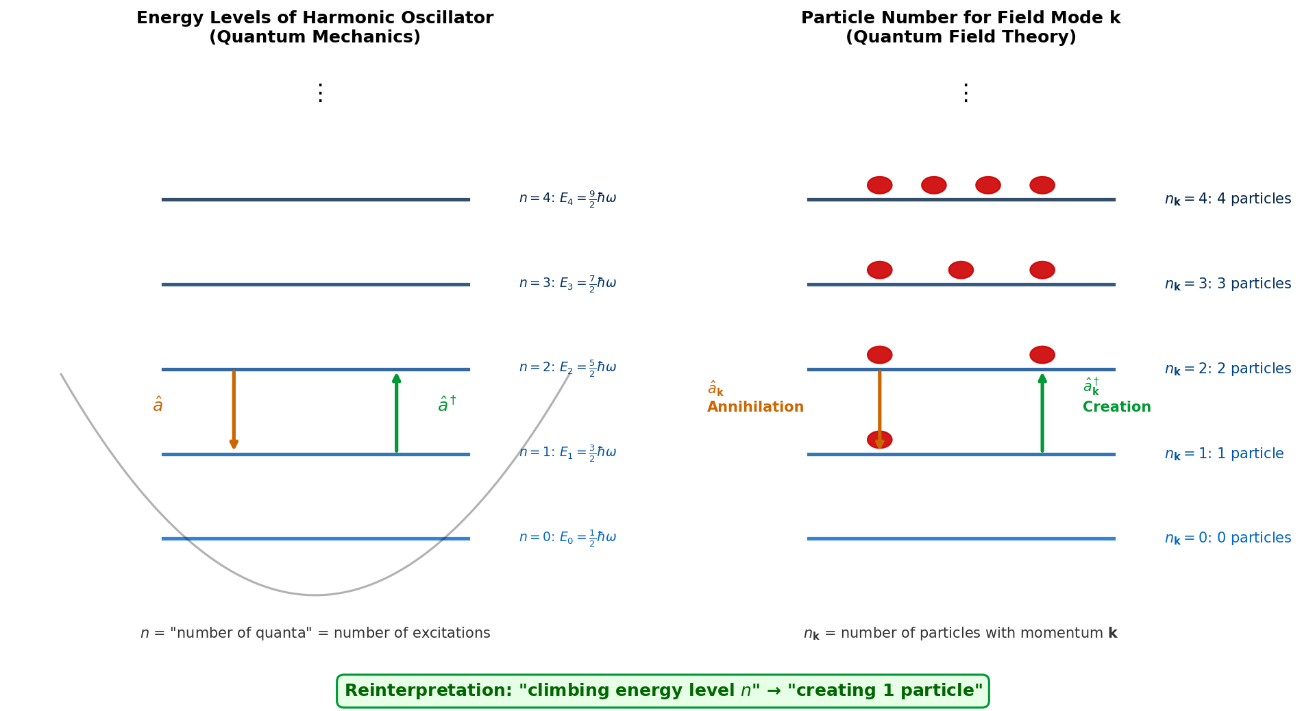
Fig. 1.12: Correspondence between harmonic oscillator energy levels and particle numbers in Fock space. Left — In a quantum mechanical harmonic oscillator, \(n\) is "the number of quanta." Right — In quantum field theory, the same \(n\) is interpreted as "the number of particles with momentum \(\mathbf{k}\)." Going up a level with the creation operator \(\hat{a}^\dagger\) corresponds to adding one particle.

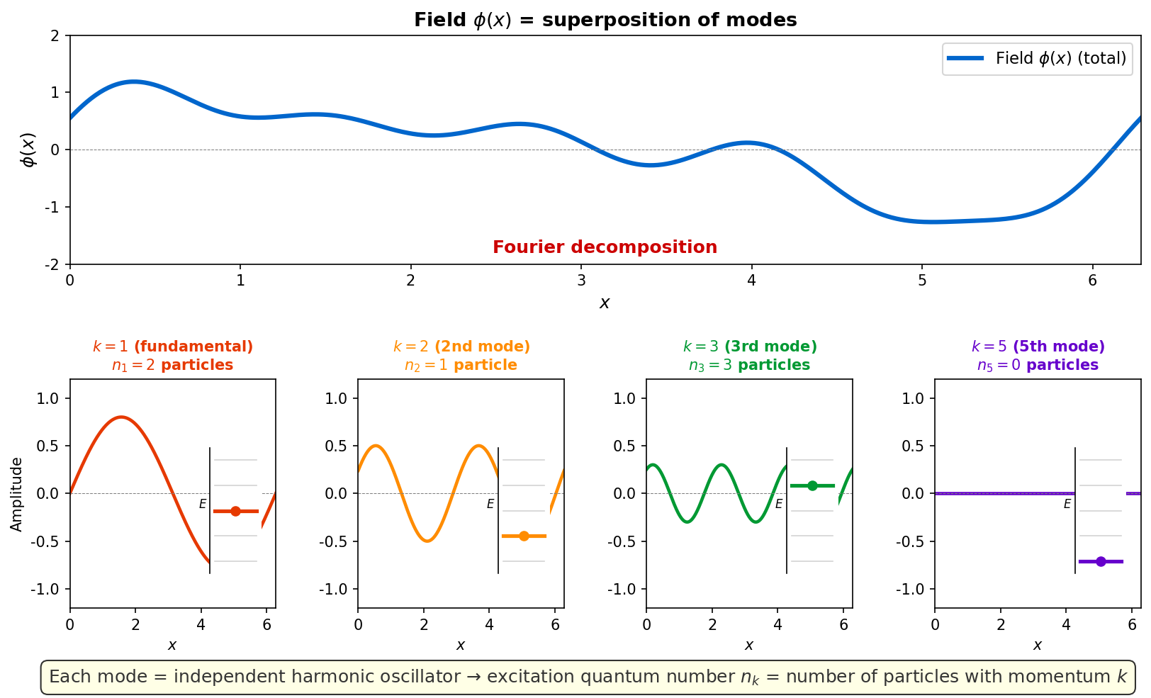
Fig. 1.13: Fourier expansion of the field and harmonic oscillator modes. Top — The field \(\phi(x)\) is a superposition of modes with various wave numbers \(k\). Bottom — Each mode corresponds to an independent harmonic oscillator, and its excitation quantum number \(n_k\) represents the particle number for that mode. The small figures on the right show energy levels, with circles indicating the current excitation state.

🟡 Lina: This is a preview of what we'll do in detail in Ch. 4. For now, just grasp the image that "the harmonic oscillator's \(\hat{a}^\dagger\) becomes an operator that creates particles."

✅ Comprehension Check: In quantum field theory, when the field is Fourier expanded, what kind of system does each mode correspond to, and what does the "quantum number \(n\)" of that mode mean?

Answer

When the field is Fourier expanded, each mode corresponds to an independent harmonic oscillator. The quantum number \(n\) of that mode is interpreted as the number of particles existing in that mode. That is, "quantum field theory = quantization of infinitely many harmonic oscillators," with each oscillator's excitation corresponding to a particle.

Fock Space — The Stage for a World Where Particle Number Changes

🟡 Lina: To describe a world where particle number changes, we also need to extend the state space. The Hilbert space used in quantum mechanics — the space where quantum mechanical state vectors \(|\psi\rangle\) live — was the state space for systems with a fixed number of particles. In quantum field theory, we extend this to Fock space.

🟡 Lina: Let me explain the construction of Fock space (see also Fig. 1.14 "Structure of Fock space"). First, define the state with 0 particles — the vacuum \(|0\rangle\). Next, prepare the 1-particle state space \(\mathcal{H}_1\) (the space spanned by states like "there is 1 particle with momentum \(\mathbf{p}\)"), the 2-particle state space \(\mathcal{H}_2\) (the space spanned by states with one particle each of momentum \(\mathbf{p}\) and \(\mathbf{q}\), or two particles of the same momentum, etc.), and so on. The Fock space is all of these combined:

\[ \mathcal{F} = \mathcal{H}_0 \oplus \mathcal{H}_1 \oplus \mathcal{H}_2 \oplus \cdots \tag{1.21} \]

🔵 Kai: What's \(\oplus\)? It's different from ordinary addition, right?

🟡 Lina: Good question. \(\oplus\) is read as direct sum. A direct sum is the operation of "combining different particle-number subspaces into one large space while keeping each one independent." In a familiar analogy, combining the \(x\)-axis and \(y\)-axis to make the \(xy\)-plane is the direct sum of two 1-dimensional spaces. The \(x\)-component and \(y\)-component are independent directions that don't interfere with each other, and any vector in the plane can be uniquely decomposed into "\(x\)-direction component" and "\(y\)-direction component," right? The direct sum does the same thing for many (possibly infinitely many) spaces. Any state in Fock space can be uniquely decomposed into "0-particle component + 1-particle component + 2-particle component + ..."

🔵 Kai: I see, the \(xy\)-plane analogy is clear. But there are infinitely many "axes," right?

🟡 Lina: That's right. Here \(\mathcal{H}_0\) is a 1-dimensional space spanned by the vacuum state \(|0\rangle\) alone, \(\mathcal{H}_1\) is the space spanned by states like "1 particle with momentum \(\mathbf{p}\)" with as many basis states as values \(\mathbf{p}\) can take (for continuous momenta it's infinite-dimensional, but for now think of it as "a large space with many basis states"). As an image, think of each space as a "room" connected by corridors to form a large building. The room for 0 particles, the room for 1 particle, the room for 2 particles... are all connected, and creation/annihilation operators serve as "doors between rooms."

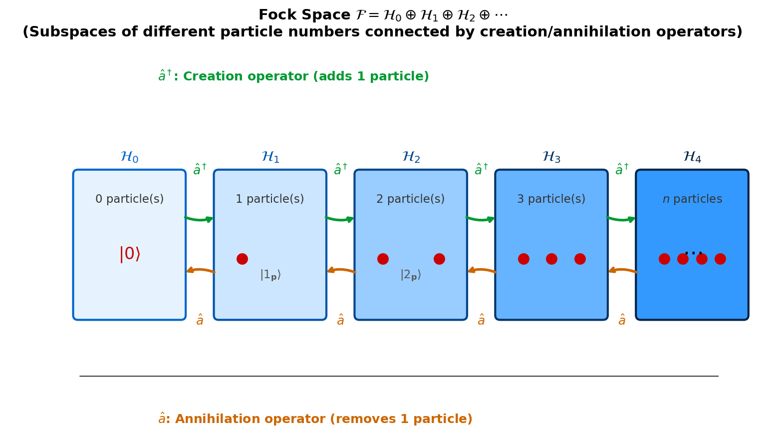
Fig. 1.14: Structure of Fock space. Each "room" \(\mathcal{H}_n\) is the space of states with \(n\) particles. The creation operator \(\hat{a}^\dagger\) adds one particle and moves to the room on the right; the annihilation operator \(\hat{a}\) removes one particle and moves to the room on the left.

🔵 Kai: I see, like combining the \(x\)-axis and \(y\)-axis, all spaces for each particle number are combined into a "big space" where physics unfolds. And since there are infinitely many rooms, Fock space is infinite-dimensional? Also, a change in particle number means moving from one "room" to another, right? Is there an operator that achieves this?

🟡 Lina: Correct, Fock space is infinite-dimensional — each "room" \(\mathcal{H}_n\) is already infinite-dimensional (since momenta take continuous values), and there are infinitely many of them. And the operators for "moving between rooms" — those are precisely the creation operator \(\hat{a}^\dagger\) and annihilation operator \(\hat{a}\). \(\hat{a}^\dagger\) adds one particle and \(\hat{a}\) removes one. That is, operators connect different particle-number subspaces.

⚪ Mei: So in quantum mechanics, operators only changed states within a space of fixed particle number, but in Fock space, creation and annihilation operators can open "doors between rooms" and change particle number.

🟡 Lina: Exactly. This is the mathematical realization of "particle creation and annihilation."

🟡 Lina: Concretely, the operator \(\hat{a}^\dagger_{\mathbf{p}}\) that creates a particle with momentum \(\mathbf{p}\):

Let me introduce the notation \(|n_{\mathbf{p}}\rangle\). This represents "the state with \(n\) particles in the mode with momentum \(\mathbf{p}\)." \(n = 0\) means no particles (vacuum), \(n = 1\) means one particle, and so on. Using this notation:

\[ \hat{a}^\dagger_{\mathbf{p}} |0\rangle = |1_{\mathbf{p}}\rangle \tag{1.22} \]

So Eq. (1.22) means "create one particle with momentum \(\mathbf{p}\) from the vacuum." In general:

\[ \hat{a}^\dagger_{\mathbf{p}} |n_{\mathbf{p}}\rangle = \sqrt{n_{\mathbf{p}}+1}\,|(n_{\mathbf{p}}+1)_{\mathbf{p}}\rangle \tag{1.23} \]

This \(\sqrt{n+1}\) coefficient has exactly the same structure as \(\hat{a}^\dagger |n\rangle = \sqrt{n+1}\,|n+1\rangle\) that we derived from commutation relations for the harmonic oscillator creation operator in Quantum Mechanics Ch. 8. If you've forgotten "why \(\sqrt{n+1}\)," review Quantum Mechanics Ch. 8. Eq. (1.22) corresponds to setting \(n_{\mathbf{p}} = 0\) in this general formula — \(\sqrt{0+1} = 1\) so the coefficient becomes 1 and is invisible. For example, substituting \(n_{\mathbf{p}} = 1\):

\[ \hat{a}^\dagger_{\mathbf{p}} |1_{\mathbf{p}}\rangle = \sqrt{2}\,|2_{\mathbf{p}}\rangle \tag{1.24} \]

The annihilation operator \(\hat{a}_{\mathbf{p}}\) conversely removes one particle:

\[ \hat{a}_{\mathbf{p}} |n_{\mathbf{p}}\rangle = \sqrt{n_{\mathbf{p}}}\,|(n_{\mathbf{p}}-1)_{\mathbf{p}}\rangle \tag{1.25} \]

Particularly important is the case \(n_{\mathbf{p}} = 0\). Substituting gives \(\hat{a}_{\mathbf{p}}|0_{\mathbf{p}}\rangle = \sqrt{0}\,|(-1)_{\mathbf{p}}\rangle = 0\) — the coefficient \(\sqrt{0} = 0\) makes the entire right side zero. So \(\hat{a}_{\mathbf{p}}|0\rangle = 0\): you cannot remove further particles from the vacuum. This corresponds to "the bottom rung of the ladder."

🔵 Kai: Oh! The harmonic oscillator's "climbing the ladder of energy levels" gets reinterpreted as "adding one particle"! And the bottom is the vacuum, which you can't go below. But if there are infinitely many harmonic oscillators, doesn't the zero-point energy \(\frac{1}{2}\hbar\omega\) from infinitely many of them diverge?

🟡 Lina: Sharp. That problem actually does exist. But let's move forward for now and tackle it head-on in Part V "Renormalization." First, let me write down the basic algebra for the boson case. To keep things simple, I'll consider the field confined in a box so that allowed momenta are restricted to discrete values (the same reason why allowed frequencies of a guitar string are discrete. The discrete case is easier to handle with sums). The creation and annihilation operators for bosons satisfy the commutation relation:

\[ [\hat{a}_{\mathbf{p}}, \hat{a}^\dagger_{\mathbf{q}}] = \delta_{\mathbf{p}\mathbf{q}} \tag{1.26} \]

For fermions, they anticommute:

\[ \{\hat{a}_{\mathbf{p}}, \hat{a}^\dagger_{\mathbf{q}}\} = \delta_{\mathbf{p}\mathbf{q}} \tag{1.27} \]

Here \(\delta_{\mathbf{p}\mathbf{q}}\) is the Kronecker delta meaning "1 when \(\mathbf{p} = \mathbf{q}\), 0 otherwise" (for discrete momenta). It's the discrete version of the Dirac delta \(\delta^3(\mathbf{x} - \mathbf{y})\) we saw earlier. For continuous momenta, it gets replaced by \(\delta^3(\mathbf{p} - \mathbf{q})\), but the essence is the same — "only the same modes have non-zero commutation relations."

🔵 Kai: What's the difference between commutation and anticommutation relations?

🟡 Lina: There's a big difference. For fermions, the creation operators also satisfy anticommutation relations: \(\{\hat{a}^\dagger_{\mathbf{p}}, \hat{a}^\dagger_{\mathbf{q}}\} = 0\). Setting \(\mathbf{p} = \mathbf{q}\) gives \(2(\hat{a}^\dagger_{\mathbf{p}})^2 = 0\), i.e., \((\hat{a}^\dagger_{\mathbf{p}})^2 = 0\). This means trying to create two particles in the same state gives zero — the Pauli exclusion principle emerges automatically.

🔵 Kai: I see, applying \(\hat{a}^\dagger_{\mathbf{p}}\) twice gives \(0\), so you can't put a second one in the same state.

⚪ Mei: The exclusion principle doesn't need to be separately assumed — it's derived from the anticommutation relation.

🟡 Lina: I've illustrated the difference in occupation numbers between bosons and fermions in Fig. 1.15 "Difference in occupation numbers between bosons and fermions. Left". The table below also contrasts their properties.

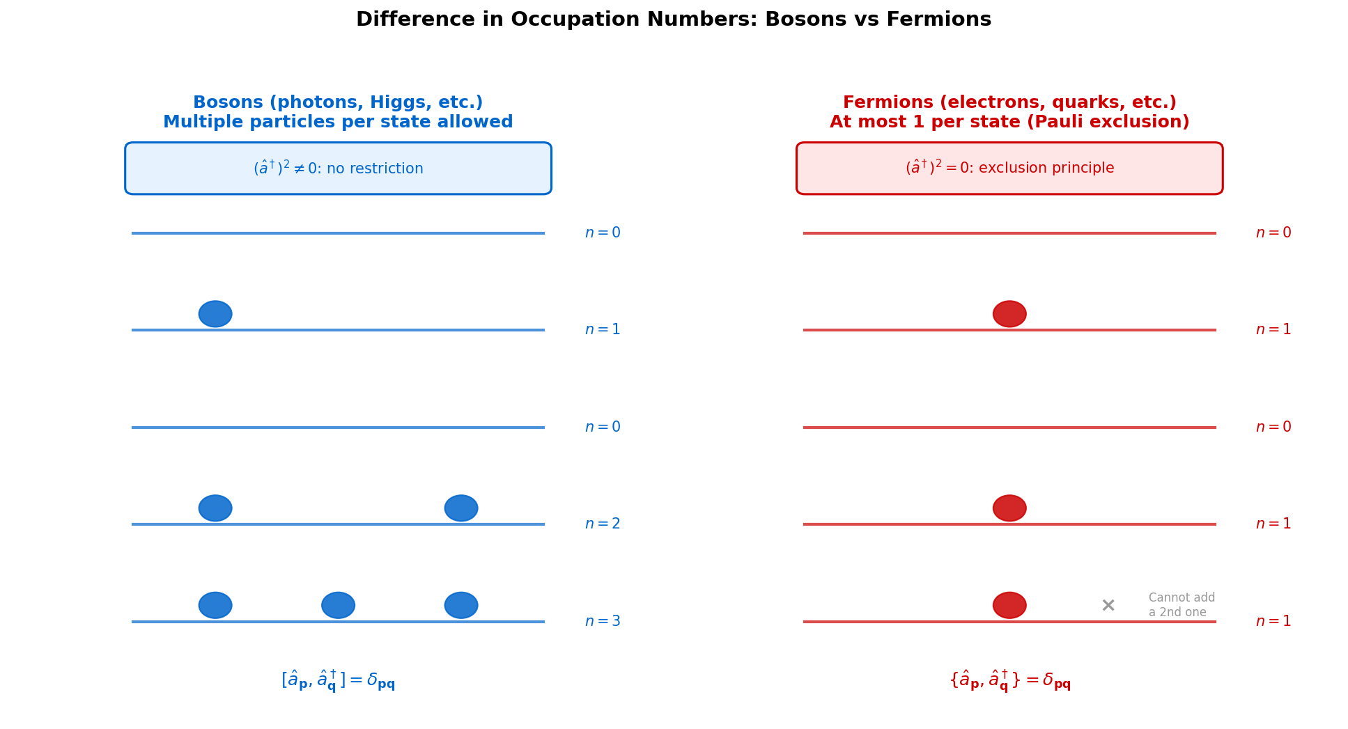
Fig. 1.15: Difference in occupation numbers between bosons and fermions. Left — Bosons satisfy commutation relations and any number of particles can occupy the same quantum state. Right — Fermions satisfy anticommutation relations and at most 1 particle can occupy each state (Pauli exclusion principle).

Table 1.7: Comparison of bosons and fermions

	Bosons (photons, Higgs particles, etc.)	Fermions (electrons, quarks, etc.)
Statistics	Bose-Einstein statistics	Fermi-Dirac statistics
Algebraic relation	Commutation relation \([\hat{a}_{\mathbf{p}}, \hat{a}^\dagger_{\mathbf{q}}] = \delta_{\mathbf{p}\mathbf{q}}\)	Anticommutation relation \(\{\hat{a}_{\mathbf{p}}, \hat{a}^\dagger_{\mathbf{q}}\} = \delta_{\mathbf{p}\mathbf{q}}\)
Occupation number	\(n = 0, 1, 2, 3, \ldots\) (no restriction)	\(n = 0, 1\) only (exclusion principle)
Spin	Integer (\(0, 1, 2, \ldots\))	Half-integer (\(1/2, 3/2, \ldots\))
Representative examples	Photons, gluons, \(W/Z\), Higgs	Electrons, quarks, neutrinos
🟡 Lina: Exactly. This is the algebraic skeleton of quantum field theory. We'll carry this out for scalar fields and Dirac fields in Ch. 4 and Ch. 5.

✅ Comprehension Check: How is the Pauli exclusion principle derived from the fact that fermionic creation operators satisfy anticommutation relations?

Answer

From the anticommutation relation \(\{\hat{a}_{\mathbf{p}}, \hat{a}^\dagger_{\mathbf{q}}\} = \delta_{\mathbf{p}\mathbf{q}}\), one can derive \((\hat{a}^\dagger_{\mathbf{p}})^2 = 0\). This means that trying to create two particles in the same state \(\mathbf{p}\) gives zero, so the Pauli exclusion principle — that no more than one fermion can exist in the same quantum state — holds automatically.

✅ Comprehension Check: State one essential way in which Fock space differs from ordinary Hilbert space.

Answer

Fock space simultaneously contains states with different particle numbers (it is the direct sum of subspaces with particle numbers 0, 1, 2, ...). Whereas ordinary Hilbert space has a fixed particle number, in Fock space the creation and annihilation operators enable operations that change particle number.

---

1.8　The Most Precise Model in Human History

🟡 Lina: Finally, let me introduce some numbers showing how successful quantum field theory is.

Among quantum field theories, the most mature is QED (Quantum Electrodynamics) — the model describing the interaction of electrons and photons. The QED theoretical prediction for the electron's anomalous magnetic moment is:

\[ a_e^{\text{theory}} = 0.001\,159\,652\,181\,78(77) \]

The experimental value is:

\[ a_e^{\text{exp}} = 0.001\,159\,652\,180\,73(28) \]

Here the numbers in parentheses represent the uncertainty in the last digits. For example, \((28)\) in the experimental value means \(\pm 28\) uncertainty in the last two digits. \((77)\) in the theoretical value means \(\pm 77\) uncertainty in the last two digits. (The theoretical value includes 5th-order (5-loop) QED corrections plus hadronic and weak force corrections. The experimental value is from precision measurements using a Penning trap. See Aoyama et al., Phys. Rev. Lett. 109, 111807 (2012) and Hanneke et al., Phys. Rev. Lett. 100, 120801 (2008) for details.)

🔵 Kai: They agree to 10 decimal places! But why is it called the "anomalous" magnetic moment? What's different from the normal magnetic moment?

🟡 Lina: Good question. The magnetic moment refers to the "strength as a tiny magnet" that the electron possesses. Since the electron has spin, as a rotating charged particle it creates a magnetic field. If we call the value predicted by the Dirac equation the "normal value," the actual value deviates slightly from it. The dimensionless quantity representing the size of that deviation is \(a_e\), called the "anomalous magnetic moment." Specifically, it's defined as \(a_e = (g - 2)/2\), where \(g\) is the "\(g\)-factor" that determines the magnetic moment's magnitude (the Dirac equation prediction learned in Quantum Mechanics Ch. 17 is \(g = 2\)). If the Dirac equation were completely correct, \(a_e = 0\). But it's not zero. The cause of the deviation is quantum corrections from the electron emitting and absorbing virtual photons — precisely the effect calculated in quantum field theory.

⚪ Mei: The Dirac equation alone isn't completely correct, and virtual photon effects produce a measurable deviation — evidence that quantum field theory is needed.

🟡 Lina: This precision is equivalent to measuring the distance from Tokyo to New York and having less than a hair's breadth of error. Quantum field theory is not just "a beautiful theory" — it's the most precisely tested physical model ever constructed by humanity.

🔵 Kai: The virtual photons that came up earlier in force mediation also cause deviations in the magnetic moment... But if virtual photons go in and out multiple times, doesn't the calculation become infinitely complicated? Adding up 1 emission/absorption, then 2, then 3... summing infinitely many should diverge, shouldn't it?

🟡 Lina: That's exactly the core difficulty of quantum field theory. Indeed, naive calculation produces infinities. But there's a systematic method for handling them — "renormalization." We'll tackle this head-on in Part V. Look forward to it.

🔵 Kai: Infinities appear but you can "handle" them to get 10-digit precision... Does "handling" infinities mean ignoring them? Or is there some other method?

🟡 Lina: Not ignoring — systematically "absorbing" them. But that's for Part V. For now, just take home the fact that "quantum field theory describes nature with astonishing precision."

🔵 Kai: Hmm, I still don't get what "absorbing" means... But conversely, if they can be handled despite diverging, there must be some regularity in "how" they diverge, right? If they diverged randomly, there'd be no way to handle them.

🟡 Lina: Sharp. That's exactly right — there's regularity in the structure of divergences. Specifically, the infinities always appear in a form that can be absorbed into redefinitions of a small number of parameters like "mass" and "charge." That's why systematic handling is possible. The true nature of this mechanism is the theme of Part V. Look forward to it.

🔵 Kai: Can be absorbed into a few parameters... So even though the infinities appear in different places each time, their "shape" always follows the same pattern? I still can't picture it at all, but I'm looking forward to Part V.

🟡 Lina: Now, looking back at what we've covered in this chapter — the breakdown of Klein-Gordon probability density, the inevitability of pair creation, the requirement of causality — all point to the same conclusion that "single-particle quantum mechanics is insufficient," and the solution is "quantize the field and describe physics in Fock space." Three independent arguments converge on the same conclusion — this is strong evidence that quantum field theory isn't "something that just happens to work" but that nature truly is this way.

⚪ Mei: It's beautiful how independent arguments point to the same conclusion. I'm looking forward to building this theory from the ground up.

✅ Comprehension Check: What is a representative physical quantity demonstrating the precision of QED (Quantum Electrodynamics)? And to what extent do theory and experiment agree?

Answer

The representative physical quantity is the electron's anomalous magnetic moment \(a_e\). The QED theoretical prediction and experimental value agree to 10 decimal places, representing the most precise agreement between theory and experiment ever achieved by humanity.

---

1.9　Roadmap for the Entire Quantum Field Theory

🟡 Lina: Finally, let's survey the overall landscape of the journey ahead spanning 24 chapters. It's divided into 7 major Parts. I've shown a visual roadmap in Fig. 1.16 "Roadmap of the entire Quantum Field Theory (24 chapters in 7 parts)".

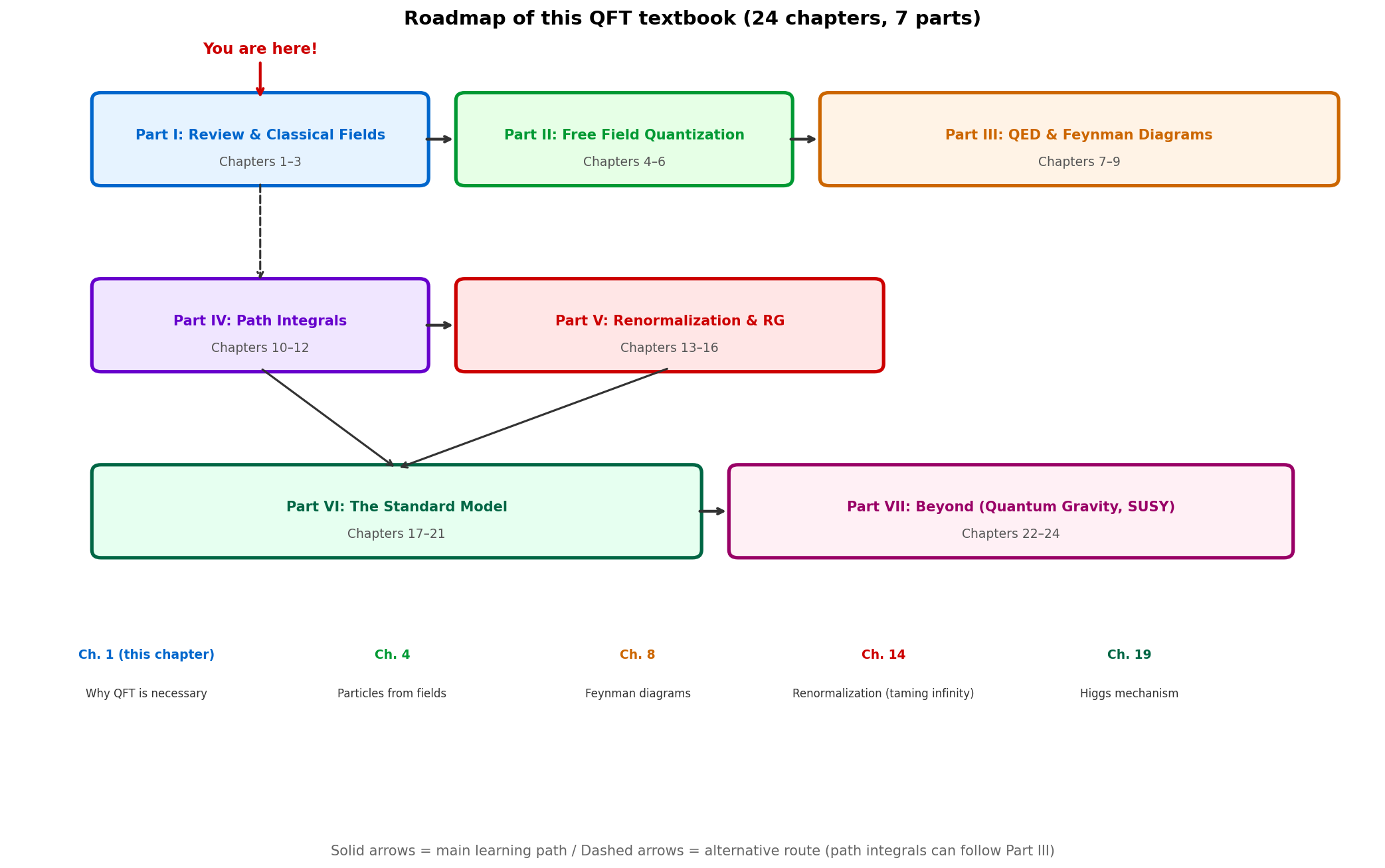
Fig. 1.16: Roadmap of the entire Quantum Field Theory (24 chapters in 7 parts). Starting from Part I (review including this chapter, and classical fields), progressing through free field quantization, QED and Feynman diagrams, path integrals, renormalization, and the Standard Model, ultimately reaching the quantum gravity problem.

Part I: Review and Classical Fields (Chapters 1–Ch. 3)

• Ch. 2 Review of special relativity and Lorentz invariance
• Ch. 3 Classical field theory (Lagrangian, Noether's theorem)

Part II: Canonical Quantization of Free Fields (Chapters 4–Ch. 6)

• Ch. 4 Quantization of the scalar field — witnessing the moment particles are born from a field
• Ch. 5 Quantization of the Dirac field — anticommutation relations for fermions
• Ch. 6 Quantization of the electromagnetic field — wrestling with gauge freedom

Part III: The First Reward — QED and Feynman Diagrams (Chapters 7–Ch. 9)

• Ch. 7 Interactions and the S-matrix
• Ch. 8 Feynman diagrams
• Ch. 9 Basic processes in QED — Rutherford scattering and Compton scattering

Part IV: Path Integrals (Chapters 10–Ch. 12)

• Ch. 10 Path integrals in quantum mechanics
• Ch. 11 Path integrals for fields and generating functionals
• Ch. 12 Path integrals for fermions (Grassmann numbers)

Part V: Renormalization and the Renormalization Group (Chapters 13–Ch. 16)

• Ch. 13 Infinities appearing inside loops
• Ch. 14 Regularization and renormalization
• Ch. 15 The renormalization group — physics that changes with scale
• Ch. 16 Effective field theory and precision tests

Part VI: The Standard Model (Chapters 17–Ch. 21)

• Ch. 17 Yang-Mills theory and gauge symmetry
• Ch. 18 Spontaneous symmetry breaking
• Ch. 19 The Higgs mechanism and the origin of mass
• Ch. 20 Electroweak unification
• Ch. 21 QCD and the completion of the Standard Model

Part VII: Beyond (Chapters 22–Ch. 24)

• Ch. 22 Applications to condensed matter (superconductivity, quantum Hall effect)
• Ch. 23 Non-perturbative phenomena (solitons, monopoles, instantons)
• Ch. 24 The quantum gravity challenge — limits of quantum field theory and the doorway to quantum gravity

🔵 Kai: What a grand journey... But today's discussion made it clear "why this journey is necessary."

⚪ Mei: To summarize: the breakdown of Klein-Gordon probability density, the inevitability of pair creation, the requirement of causality — three independent arguments all demand "field quantization," and the stage for this is Fock space. From here on, it's a journey of concretely building this framework.

🟡 Lina: Exactly. Once you understand "why," you'll always be able to understand "how." In the next chapter, we'll first prepare the tools of special relativity and get comfortable with Lorentz covariant notation.

---

Preview of Next Chapter

Ch. 2 Review of Special Relativity and Lorentz Invariance

To formulate quantum field theory, a "language" for freely manipulating Lorentz invariance is indispensable. In the next chapter, we organize 4-vectors, Lorentz transformations, the metric tensor \(\eta_{\mu\nu}\), and the distinction between covariant and contravariant, building skill in writing physical quantities with indices. We restructure the content of General Relativity Chapters 3–4 for QFT use. Once comfortable with this notation, you'll be able to verify at a glance that "all equations appearing in later chapters are Lorentz invariant."

Practice Problems

📝 Exercises:

• Calculation of Klein-Gordon probability density → Problem M-1. Lorentz Covariance of the Probability Current Density for the Klein-Gordon Equation
• Compton wavelength and the uncertainty principle → Problem B-5. Calculation of the Compton Wavelength
• Compton wavelength and the scale of pair creation → Problem M-3. Compton Wavelength and Position Localization
• Threshold energy for pair creation → Problem B-7. Time Scale of Pair Creation from the Uncertainty Relation

References

• Lancaster & Blundell, Quantum Field Theory for the Gifted Amateur Chapter 1 "What is quantum field theory?"
• Sakamoto Masato, Quantum Field Theory — Focusing on Invariance and Free Fields Chapter 8 "Fields and particles"
• Schwartz, Quantum Field Theory and the Standard Model Chapter 1 "Microscopic theory of radiation"
• Tong, Lectures on Quantum Field Theory Chapter 1 "Classical Field Theory" introduction

← Welcome to This JourneyCh. 2 Review of Special Relat… →

Feedback on this page

Let us know if something was unclear, incorrect, or could be improved.

Submit