Chapter 2 Blueprint of the Journey — Tensors and the Big Picture of the Einstein Equation
Story so far: In Ch. 1, we rewrote Newton's gravity model in the language of "field theory" and identified two limitations — the perihelion precession of Mercury and the structural problem that the Poisson equation lacks time derivatives. To resolve this contradiction with special relativity's principle that "no signal can travel faster than light," we need to rethink the foundations of Newton's model: "absolute time" and "absolute space."
Goals of This Chapter
- This chapter lays out the blueprint of the long journey from special relativity to general relativity
- Detailed derivations of individual equations will come step by step in later chapters, but grasping "where we're headed" first prevents getting lost on the mountain path along the way
- In this chapter, we introduce the tool for writing physical laws that don't depend on the choice of coordinates — tensors — and survey how Einstein's gravity model is built on two pillars: the equation of motion for particles (geodesic equation) and the field equation (Einstein equation)
- Starting from the next chapter, we'll concretely construct the first piece of this blueprint (rank-0 tensor = spacetime interval \(ds^2\))
2.1 Scalars, Vectors, and Tensors
🟡 Lina: Let's begin with the most important idea for studying relativity. A physical model must not depend on the choice of coordinate system. Whether we place the origin in Tokyo or Paris, the laws of physics should take the same form — this is the demand of the principle of relativity.
🔵 Kai: But the coordinate components \((x, y, z)\) change depending on where we place the origin and how we orient the axes. For example, depending on whether the origin is at the corner of the classroom or at the teacher's desk, the same desk's position could be \((3, 2, 0)\) or \((1, -1, 0)\).
🟡 Lina: That's right. But the distance between two desks doesn't change no matter where you place the origin or how you rotate the coordinate axes, does it?
🔵 Kai: True. The components change, but the distance doesn't.
🟡 Lina: Now what about vectors? Even in high school physics, the components \((v_x, v_y, v_z)\) of a vector (an arrow) change with the orientation of the coordinate axes, but the arrow itself stays the same, right?
⚪ Mei: Right. What distance and vectors have in common is that "the components change with the coordinate system, but the quantity itself doesn't change" — there's something essential that doesn't depend on the choice of coordinates.
🟡 Lina: Exactly. To organize this,
- A quantity like distance, whose value itself doesn't change under coordinate transformations → scalar (invariant)
- A quantity like an arrow, whose components change but whose rule of change (such as multiplying by a rotation matrix) is fixed → vector
The generalization of these is the tensor — a collective term for quantities whose components change according to a fixed rule under coordinate transformations. The specific content of "fixed rule" will be formally studied in Ch. 6, so for now just think of it as "a quantity whose components change according to a definite law."
🔵 Kai: So scalars and vectors are both members of the tensor family, and the difference is "how many times you apply the rule"?
🟡 Lina: Exactly right. Roughly speaking, a scalar doesn't change value even under transformation, a vector has its components change by applying the coordinate transformation rule once, a rank-2 tensor applies the same rule twice (once for each index) — the number of times you apply the rule increases with the number of indices.
⚪ Mei: The transformation gets more complex as the number of indices increases, but the idea is the same.
🟡 Lina: For example, when you rotate the coordinate axes by 30°, each component of a vector changes by multiplying the rotation matrix once to get the new components. A rank-2 tensor has the rotation matrix applied to both the row and column of each entry in its \(4 \times 4\) table — that is, applied twice. Let me put in a figure showing how tensors of each rank behave when you rotate the coordinate axes (Fig. 2.1 "Behavior of tensors of each rank under coordinate transformations (rotations). Left").
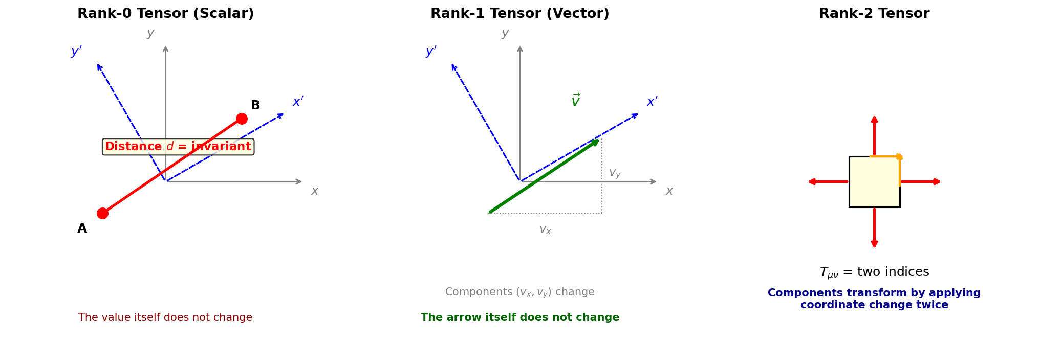
Fig. 2.1: Behavior of tensors of each rank under coordinate transformations (rotations). Left — Rank 0 (scalar): the distance between two points doesn't change no matter how you rotate the axes. Center — Rank 1 (vector): components \((v_x, v_y)\) change with the orientation of axes, but the arrow itself is the same. Right — Rank-2 tensor: components change by applying the coordinate transformation "twice."
An equation written in terms of tensors, if it holds in one coordinate system, holds in the same form in all coordinate systems.
✅ Comprehension Check: Why are equations written in terms of tensors suitable for describing physical laws?
Answer
Because an equation written in terms of tensors, if it holds in one coordinate system, holds in the same form in all coordinate systems. This allows us to express physical laws that don't depend on the choice of coordinate system.
🔵 Kai: What are tensors, concretely?
🟡 Lina: Tensors have a "rank," classified by the number of indices they carry.
🔵 Kai: Indices — like the \(\mu\) in \(U^\mu\)?
🟡 Lina: Yes. An index is a "label specifying a component." For example, a 3-dimensional vector \(\vec{v}\) has three components \((v_x, v_y, v_z)\), right? If we write this as \(v^i\) (\(i = 1, 2, 3\)), the index \(i\) specifies "which component." In relativity, we consider 4-dimensional spacetime adding 1 time dimension to 3 spatial dimensions, so the index takes four values \(\mu = 0, 1, 2, 3\), where \(0\) corresponds to time and \(1, 2, 3\) correspond to space. One index means 4 components, two indices mean \(4 \times 4 = 16\) components, and so on.
Table 2.1: Tensor rank and examples
| Rank | Number of indices | Name | Familiar example | Examples appearing later |
|---|---|---|---|---|
| Rank 0 | None | Scalar (invariant) | Distance between two points | Spacetime interval \(ds^2\) (Chapter 3~), proper time \(d\tau\) |
| Rank 1 | 1 | Vector | Force \(\vec{F}\), velocity \(\vec{v}\) | 4-velocity \(U^\mu\), 4-momentum \(p^\mu\) |
| Rank 2 | 2 | Rank-2 tensor | (Doesn't appear in high school, but something like a \(4 \times 4\) table = matrix. Physical example: stress describing stretching/compression in various directions) | Metric \(g_{\mu\nu}\) (Chapter 6~), \(T_{\mu\nu}\) (Chapter 14~) |
⚪ Mei: So scalars and vectors are both special cases of tensors.
✅ Comprehension Check: What determines the "rank" of a tensor?
Answer
It's determined by the number of indices it carries. Rank 0 (no indices) is a scalar, rank 1 (one index) is a vector, rank 2 (two indices) is a rank-2 tensor.
📝 Exercises:
- Identifying tensor ranks of physical quantities → Problem B-1. Determining the Tensor Rank of Physical Quantities
2.2 From Newton's Equation of Motion to 4-Vectors
🟡 Lina: As a familiar example, Newton's equation of motion \(\vec{F} = m\vec{a}\) is an equation written in terms of vectors (rank-1 tensors). No matter how you rotate the coordinate axes, it holds in the same form — because it's written in vector form, invariance is automatically guaranteed.
🔵 Kai: In high school, we split the equation of motion into \(x\)- and \(y\)-components as \(F_x = ma_x\), \(F_y = ma_y\). But back then, I never thought about how \(F_x\) would change if we changed the orientation of the axes.
🟡 Lina: That's the point. In high school, once you chose one set of coordinate axes, you just proceeded with the calculation, so there was no need to ask "what if we used a different coordinate system?" But in relativity, we demand that the laws of physics take the same form across different inertial frames.
🔵 Kai: What's an inertial frame?
🟡 Lina: A coordinate system that's neither accelerating nor rotating. Intuitively, it's "the viewpoint of an observer who isn't subject to any force." Using a train analogy: inside a train moving at constant speed, and on the platform at a station — both are inertial frames. A train that's accelerating or going around a sharp curve is not an inertial frame.
To put it a bit more physically, it's a coordinate system in which an object with no forces acting on it continues in uniform straight-line motion. Since Newton's first law — the law of inertia — holds as-is in such a system, it's called an "inertial frame." Conversely, inside an accelerating train, an object with no forces on it (say, a can of coffee placed on the seat) appears to start moving on its own — this is not an inertial frame. Also, any other coordinate system moving in uniform straight-line motion relative to a given inertial frame is also an inertial frame. There isn't just one inertial frame — there are infinitely many. Let me summarize this in a figure (Fig. 2.2 "Difference between inertial and non-inertial frames. Left and center").
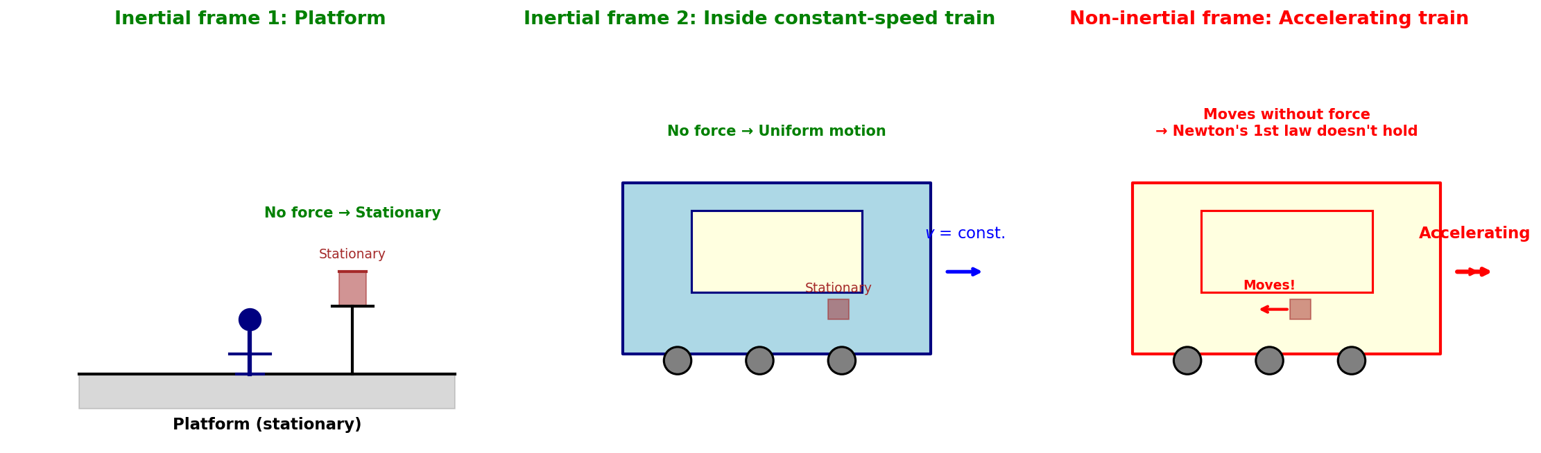
Fig. 2.2: Difference between inertial and non-inertial frames. Left and center — Both the platform and a train moving at constant speed are inertial frames: objects with no forces on them remain at rest or continue in uniform straight-line motion. Right — An accelerating train is a non-inertial frame: a can of coffee with no forces on it appears to start moving on its own (the law of inertia doesn't hold).
🔵 Kai: I see — inside a train moving at constant speed and on the platform are both inertial frames, but an accelerating train isn't. You determine it by whether an object with no forces on it continues in uniform straight-line motion.
🟡 Lina: Exactly. And since \(\vec{F} = m\vec{a}\) is written in vector form, the form of the equation doesn't change no matter how you rotate the coordinate axes — vectors automatically guarantee invariance.
⚪ Mei: This connects to the tensor discussion earlier. A vector is a rank-1 tensor, so even though its components change according to the transformation rules, the form of the equation is preserved.
🔵 Kai: Is it the same not just for rotations but also for where you place the origin?
🟡 Lina: Yes. \(\vec{F} = m\vec{a}\) involves not position itself but acceleration (the second derivative of position), so shifting the origin has no effect. In other words, it's invariant under both spatial rotations and translations.
🔵 Kai: What about changing the scale of the coordinate axes — say, from meters to centimeters?
🟡 Lina: Since both sides of \(\vec{F} = m\vec{a}\) have the same dimensions (units), changing meters to centimeters scales both sides by the same factor, and the equality still holds. So it's invariant under rescaling too.
🔵 Kai: Then what happens in an accelerating coordinate system?
🟡 Lina: At the stage of special relativity, we write equations whose form doesn't change between inertial frames (coordinate systems in uniform straight-line motion). To handle accelerating coordinate systems, we need the framework of general relativity. In general relativity, the equations can be written in the same form in any coordinate system, whether accelerating or rotating. We'll see this step by step in later chapters.
🔵 Kai: The same form in any coordinate system — that's amazing. But then, what was the reason for restricting to inertial frames in special relativity? Couldn't we just use general relativity from the start?
🟡 Lina: The mathematical tools for general relativity are far more complex. First understanding special relativity, which holds only in inertial frames, and then generalizing step by step — that makes the physical essence easier to see. In fact, our journey ahead follows that same order.
🔍 Dive Deep: If written in tensors, isn't it invariant under all coordinate transformations?
(This note contains somewhat advanced content. Feel free to skip it and come back after later chapters.)
You might wonder: "If equations written in tensors don't change form under any coordinate transformation, why is special relativity restricted to inertial frames?"
Actually, the form of a tensor equation indeed doesn't change under any coordinate transformation. The issue isn't the form but the physical assumptions contained in the equation.
Special relativity assumes that spacetime is flat. The tool that determines "how spacetime is measured" — the metric tensor — takes the form of a specific constant matrix in inertial frames (its specific content is introduced in Ch. 4). This assumption holds only in inertial frames. When you switch to an accelerating coordinate system, the components of the metric tensor vary with location and time, and the situation can no longer be described as "flat spacetime."
In general relativity, we write equations from the start using a general metric tensor that varies from place to place. That's why the same form holds in any coordinate system. This is called general covariance. For now, just keep in mind that "in general relativity, equations hold in the same form even in non-inertial frames." The specific form of the metric tensor is studied in Ch. 4, and general coordinate transformations from Ch. 6 onward.
🟡 Lina: Combining the earlier explanation with the Dive Deep supplement, special relativity covers only inertial frames, while general relativity ensures the form of equations doesn't change in any coordinate system — the scope of coverage expands. Let me put it in a table.
Table 2.2: Scope of coordinate transformations handled by special and general relativity
| Special Relativity | General Relativity | |
|---|---|---|
| Transformations under which invariance is guaranteed | Transformations between inertial frames (Lorentz transformations) | Any coordinate transformation |
| Assumption about spacetime | Flat (no acceleration or gravity) | May be curved |
| Situations it cannot handle | Accelerating coordinate systems, gravity | None (handles everything) |
| Metric tensor | Constant matrix (independent of location) | Varies from place to place |
🔵 Kai: \(\vec{F} = m\vec{a}\) is written in vectors (tensors), so it's already in a coordinate-independent form, right? Isn't that sufficient?
🟡 Lina: For "spatial" rotations and translations, yes. But in special relativity, from the viewpoint of an observer moving at near light speed, time and space mix together into a concept called spacetime — we'll look at this in detail in Ch. 3. The \(\vec{F}\) and \(\vec{a}\) in \(\vec{F} = m\vec{a}\) are 3-dimensional spatial vectors, so they can handle spatial rotations, but they cannot handle switching between inertial frames (transformations that mix time and space). Illustrating this difference (Fig. 2.3 "Coverage of 3-dimensional vectors versus 4-vectors. Left"),
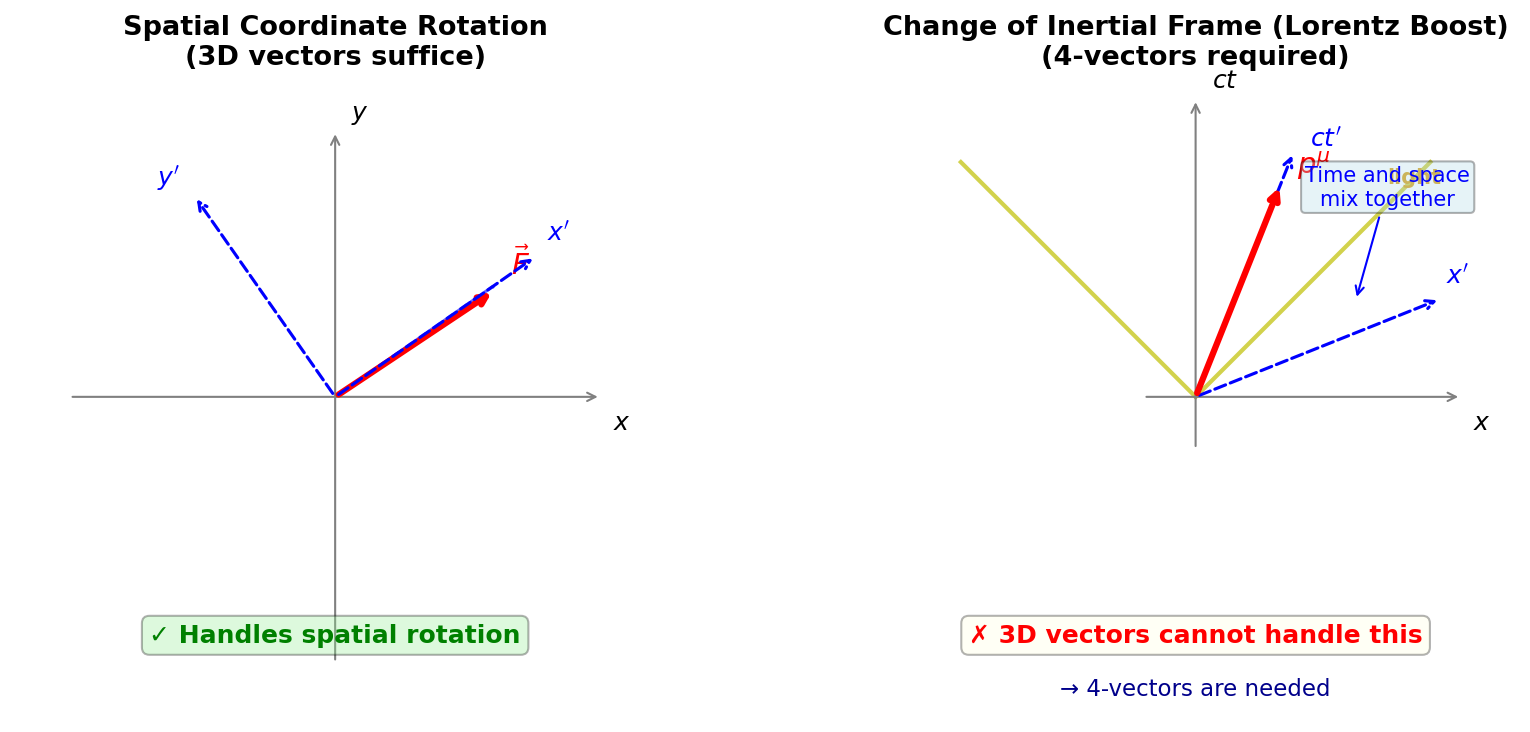
Fig. 2.3: Coverage of 3-dimensional vectors versus 4-vectors. Left — Under spatial coordinate rotation, only the components of 3-dimensional vectors change and the equation's form is preserved. Right — When switching inertial frames (Lorentz transformation), time and space axes mix, so 3-dimensional vectors cannot describe this. 4-vectors with a time component are needed.
Therefore, we need to extend to 4-dimensional vectors — 4-vectors (rank-1 tensors) — by adding a time component. The relativistic version of Newton's equation of motion is
🔵 Kai: Oh, it looks very similar to Newton's equation. \(\vec{F}\) becomes \(f^\mu\) and \(\vec{a}\) becomes \(\frac{d^2 x^\mu}{d\tau^2}\) — that's it?
🟡 Lina: Yes, compare it with Newton's \(\vec{F} = m\vec{a} = m\frac{d^2 \vec{r}}{dt^2}\). The force \(\vec{F}\) corresponds to the 4-force \(f^\mu\), and the acceleration \(\frac{d^2 \vec{r}}{dt^2}\) corresponds to \(\frac{d^2 x^\mu}{d\tau^2}\) — the 3-dimensional position \(\vec{r}\) is replaced by the 4-dimensional coordinate \(x^\mu\), and the absolute time \(t\) is replaced by the proper time \(\tau\). The index \(\mu\) (mu) takes four values \(0, 1, 2, 3\). \(x^1, x^2, x^3\) correspond to spatial coordinates \(x, y, z\), and \(x^0\) is the coordinate related to time (its specific definition is introduced in Ch. 3). In other words, this single equation simultaneously represents four equations for time and space. And this equation doesn't change form when you switch inertial frames.
Note on notation: The \(\tau\) (tau) in the denominator is the proper time — the time ticked by a clock moving along with the particle. In Newtonian mechanics, time is the same for all observers (absolute time), so there was only \(t\). But in special relativity, each observer's time ticks differently, so we need to distinguish between the particle's own clock time \(\tau\) and the coordinate time \(t\) as seen from a given inertial frame. The precise definition and its relationship to \(t\) are introduced in Ch. 3, so for now think of it as "the relativistic rewriting of Newton's \(t\)."
✅ Comprehension Check: Why is it necessary to extend Newton's equation of motion to 4-vectors? What is insufficient about the 3-dimensional vector form \(\vec{F} = m\vec{a}\)?
Answer
3-dimensional vectors are invariant under spatial rotations, but in special relativity they cannot handle switching between inertial frames (Lorentz transformations) where time and space mix. By extending to 4-vectors with a time component, the equation's form remains unchanged even when switching inertial frames.
🔵 Kai: I understand that \(\mu = 1, 2, 3\) correspond to Newton's \(F_x = ma_x\) and so on. But what does the time component \(\mu = 0\) represent?
🟡 Lina: The \(\mu = 0\) component becomes an equation related to energy. The time component of the 4-force corresponds to the rate of change of the particle's energy — that is, the power. The details will be derived in Ch. 4 when we study 4-vectors, so for now just remember that "extending from 3 to 4 dimensions unifies the law of motion and the law of energy into a single equation."
⚪ Mei: So \(\mu = 1, 2, 3\) are the spatial equations of motion, and \(\mu = 0\) is the energy equation — both are contained within a single equation.
🟡 Lina: Right. When time and space become unified, the law of motion and the law of energy merge into one equation — that's the beauty of special relativity. \(E = mc^2\) also emerges naturally from this structure.
🔵 Kai: \(E = mc^2\) comes out naturally? How...?
🟡 Lina: It comes from calculating the "length" of the 4-momentum vector. The specific derivation is in Ch. 4, so look forward to it.
🔵 Kai: The "length" of a vector... In 3 dimensions it's \(|\vec{v}| = \sqrt{v_x^2 + v_y^2 + v_z^2}\), but in 4 dimensions the time component is included, so it must be something different. I'll look forward to it. ...But what I'm curious about is, this 4-vector equation \(f^\mu = m\frac{d^2 x^\mu}{d\tau^2}\) has the structure "if the force is given, the motion is determined," right? If we try to put gravity into \(f^\mu\), wouldn't that just be rewriting Newton's gravity in 4 dimensions? Would that solve the problems from Ch. 1?
🟡 Lina: Good question. Actually, to handle gravity requires one more leap. Let's look at that in the next section.
✅ Comprehension Check: When extending Newton's equation of motion \(\vec{F} = m\vec{a}\) to special relativity, we need to promote 3-dimensional vectors to 4-vectors. What does the additional \(\mu = 0\) component physically correspond to?
Answer
It corresponds to the energy equation (power). When time and space become unified, the law of motion and the law of energy merge into a single equation.
📝 Exercises:
- Why 3-dimensional spatial vectors alone are insufficient → Problem B-2. Limitations of Newton's Equation of Motion
2.3 Gravity Is Not a Force but Curvature of Spacetime
🔵 Kai: Then isn't this solved? If we rewrite Newton's equation of motion using 4-vectors, don't we get an equation of gravity consistent with relativity?
🟡 Lina: Good question, but actually that's not enough. This equation determines "how a particle moves when a force \(f^\mu\) is given." The problem is how to put gravity into the force on the left-hand side.
🔵 Kai: Can't we just put Newton's gravity \(F = -GMm/r^2\) into \(f^\mu\)? Just rewriting the form as a 4-vector.
🟡 Lina: That's the natural idea. But as we saw in Ch. 1, Newton's gravity was "instantaneous action at a distance." Even if you rewrite the form as a 4-vector, the mechanism of propagation itself doesn't change — as long as you treat gravity as a "force," the problem of "how that force propagates" persists. This is where Einstein's revolutionary insight comes in.
⚪ Mei: So just rewriting the form of the force relativistically doesn't eliminate the structural problem.
🟡 Lina: Exactly. Einstein's answer was to describe gravity not as a force but as curvature of spacetime. The curvature of spacetime is determined by the field equation (Einstein equation), and that equation is consistent with special relativity — meaning changes in spacetime curvature propagate at or below the speed of light \(c\). These are gravitational waves. The "instantaneous propagation" problem is naturally resolved by describing gravity through a field equation.
And in curved spacetime, a particle simply travels along a geodesic (the "straightest possible path" in curved spacetime) without receiving any force. Gravity is absorbed into the geometry of spacetime rather than being a force.
Supplement: Some textbooks explain "geodesic" as "shortest path," but more precisely it's a stationary path — a path for which a certain quantity doesn't change when the path is slightly varied. Recall the principle of least action from Ch. 1: the path that satisfies the variation \(\delta S = 0\) of the action \(S\) is the realized path. Geodesics have the same structure: "a path for which the variation of proper time is zero." In high school you learned about maxima and minima of \(y = f(x)\) — those are "points where the derivative is zero — meaning points where \(y\) doesn't change even if you shift \(x\) slightly." Here we apply the same idea to "paths": "a path for which the change in proper time is (to first order) zero even when the path is slightly varied" is a geodesic. It has the same structure as the principle of least action from Ch. 1. In the geometry of space alone, geodesics are shortest paths, but in spacetime geometry the situation differs — for massive particles, geodesics are paths that maximize proper time. Intuitively, "the more you detour, the shorter your proper time becomes," so the straight geodesic gives the maximum. "Detours making time shorter" contradicts everyday intuition, but this is the same phenomenon as "time dilation" in special relativity — a moving clock runs slower, meaning the more a particle moves around (detours), the less time its own clock (proper time) accumulates — we'll study this in detail in Ch. 3.
🔵 Kai: Can a particle curve without any force?
🟡 Lina: To understand that, let me introduce the spacetime diagram perspective. It's a diagram with spatial coordinates \((x, y)\) on the horizontal axes and time on the vertical axis. The trajectory that an object traces on a spacetime diagram is called a world line — whether at rest or in motion, time flows, so every object extends its trajectory upward (toward the future) on the diagram.
🔵 Kai: The vertical axis is labeled \(ct\) — why \(ct\) instead of \(t\)?
🟡 Lina: The spatial axes are in meters, but if the time axis were in seconds, the dimensions would differ and we couldn't draw them on the same diagram. So we use \(ct\), which is time \(t\) multiplied by the speed of light \(c\). Since \(c \times t\) is "the distance light travels in \(t\) seconds," its unit is meters — the same dimension as space. Let's look at the diagram (Fig. 2.4 "Geodesics in flat and curved spacetime. The vertical axis is time \(ct\), and the two horizontal axes \((x, y)\) are space. Left").
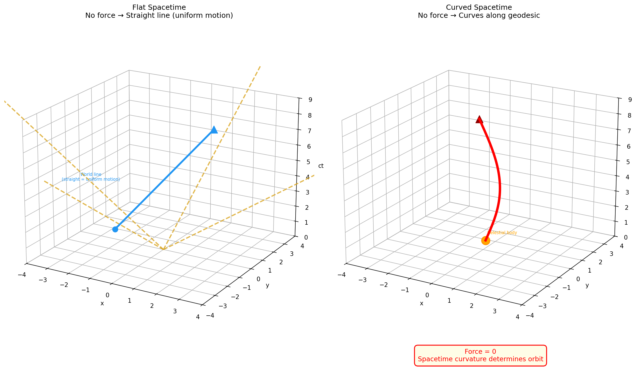
Fig. 2.4: Geodesics in flat and curved spacetime. The vertical axis is time \(ct\), and the two horizontal axes \((x, y)\) are space. Left — In flat spacetime, a particle with no force on it traces a straight world line in spacetime. This corresponds to uniform straight-line motion. Right — In curved spacetime around a celestial body, the world line curves even without any force. This is a geodesic — "straight" in curved spacetime. The yellow dashed lines are light world lines (cross-sections of the light cone, at 45° lines), and world lines of massive particles are steeper than these (not exceeding the speed of light).
🟡 Lina: The key point is that all objects inevitably advance in the time direction (upward along the \(ct\) axis). Whether at rest or in motion, time flows — in the spacetime diagram, this corresponds to the object's trajectory extending in the \(ct\) direction.
⚪ Mei: A stationary object's world line goes straight up along the \(ct\) axis. An object in uniform straight-line motion also shifts in the spatial direction at a constant rate, so it becomes a tilted straight line.
🟡 Lina: Exactly. The left side of the figure shows precisely that. The blue straight line is the world line of a particle in uniform straight-line motion — as time passes, the spatial position shifts at a constant rate, making it a tilted straight line. Since no force is acting, the world line doesn't curve.
🔵 Kai: How do I read the right side?
🟡 Lina: The right side shows the case where spacetime is curved. Even without any force, as the particle advances in the \(ct\) direction, it shifts in the spatial direction — the world line curves. What's curved isn't the particle's trajectory but spacetime itself. The particle is just going straight (along a geodesic) in the curved spacetime. It's the same idea as how walking "straight" on the Earth's surface still traces a curve because the Earth is round.
Also, did you notice the yellow dashed lines in the figure? Those are the trajectories of light — light's world lines. Since the spatial axes and the \(ct\) axis have the same units, light traces straight lines at 45°. Massive particles are slower than light, so their world lines go in a direction steeper than 45° (closer to the \(ct\) axis). The cone formed by these 45° lines is called the light cone. We'll study it in detail in Ch. 3.
🔵 Kai: How do you write "going straight in curved spacetime" in equations?
🟡 Lina: In Newton's equation of motion with zero force \(\vec{F} = 0\), we get \(\vec{a} = 0\) — meaning uniform straight-line motion. This is "straight in flat space." Extending to 4 dimensions gives \(\frac{d^2 x^\mu}{d\tau^2} = 0\) — zero acceleration. But when spacetime is curved, the very meaning of "straight" changes. In curved spacetime, having zero coordinate acceleration doesn't necessarily mean truly straight, and conversely, what appears as acceleration in coordinates might actually be straight in spacetime.
🔵 Kai: Accelerating in coordinates but actually straight...? That sounds like a paradox.
🟡 Lina: For example, a freely falling apple appears to accelerate at \(g\) in the ground-based coordinate system, but in Einstein's view it's receiving no force — it's just going straight along a geodesic in curved spacetime. Conversely, it's us standing on the ground who are being accelerated by a force (the normal force from the ground) — meaning we are the ones deviating from the "straight path in curved spacetime" (geodesic).
So to determine whether something is "truly going straight" in curved spacetime, the coordinate acceleration \(\frac{d^2 x^\mu}{d\tau^2}\) alone isn't enough — we need a correction term that accounts for the curvature and distortion of the coordinate system itself. This correction term depends on the particle's velocity (which direction and how fast it's going).
Think about it on the Earth's surface. Walking east along the equator follows a line of latitude — it looks straight on a map but is actually curved. On the other hand, walking north from the same location follows a meridian — the curvature is different. So "which direction you're going" changes how the correction works. Furthermore, walking diagonally northeast involves both the northward and eastward components — the correction is determined by the combination of "how much you're going north" and "how much you're going east."
⚪ Mei: So the magnitude of the correction changes with both "the direction of travel" and "the speed of travel."
🟡 Lina: Exactly. In 4-dimensional spacetime it's the same — all combinations of velocity in the \(\alpha\) direction and velocity in the \(\beta\) direction (where \(\alpha, \beta\) each run over \(0, 1, 2, 3\)) contribute to the correction. To give an intuitive reason for why it's a "product": when walking diagonally northeast, the correction is simultaneously proportional to both "how much you're going north" and "how much you're going east" — if either is zero, the diagonal correction vanishes too, so it takes the form of multiplication rather than addition. For example, if the northward velocity is \(v_N\) and the eastward velocity is \(v_E\), the diagonal-specific correction is proportional to \(v_N \times v_E\). Walking due north (\(v_E = 0\)) gives zero diagonal correction; walking due east (\(v_N = 0\)) also gives zero — it only matters when both are simultaneously nonzero. Of course, even when walking due north, there's still a correction for the north direction itself (a term proportional to \(v_N \times v_N\)) — including cases where \(\alpha\) and \(\beta\) are the same direction, we sum over all combinations.
🔵 Kai: I see, so products of the same direction and products of different directions are all included. In 4 dimensions there must be many combinations...
🟡 Lina: Right, since \(\alpha\) and \(\beta\) each run over \(0, 1, 2, 3\), it becomes a sum of \(4 \times 4 = 16\) terms. In equation form it's \(\Gamma^\mu_{\alpha\beta}\frac{dx^\alpha}{d\tau}\frac{dx^\beta}{d\tau}\) (where \(\Gamma^\mu_{\alpha\beta}\) is a coefficient representing "the strength of correction at each location" — I'll explain its content shortly). Written explicitly with the \(\Sigma\) (sigma) symbol, it means \(\sum_{\alpha=0}^{3}\sum_{\beta=0}^{3}\Gamma^\mu_{\alpha\beta}\frac{dx^\alpha}{d\tau}\frac{dx^\beta}{d\tau}\). In relativity we omit this \(\Sigma\) and write with the convention that "whenever the same index appears once upstairs and once downstairs, sum over it" — I'll formally explain this shorthand notation (Einstein's summation convention) a bit later.
🔵 Kai: Wait, the person standing on the ground is accelerating? Even though they're not moving?
🟡 Lina: It seems strange by everyday intuition. But remember — if you hold an accelerometer (there's one in your smartphone) while in free fall, the accelerometer reads zero. That's because the springs and sensors inside the accelerometer are falling along with you, so the spring doesn't compress = no force is detected. Conversely, when standing on the ground, the accelerometer shows \(g\) pointing upward — because the ground is pushing the sensor up. So "truly receiving no force (zero acceleration)" applies to the falling apple, while the person standing on the ground is constantly being pushed up by the normal force — that's Einstein's perspective. "Acceleration" here means deviating from the geodesic (the straight path in curved spacetime) — the person on the ground is continually being deflected from the free-fall path by the normal force. We'll dig deeper into this in Ch. 5 when we study the equivalence principle. What matters here is that the apple "appearing to accelerate" in the ground-based coordinate system is because the coordinate system itself is accelerating (being pushed by the ground). The \(\Gamma\) term is what handles this correction. As a result, "straight in curved spacetime" — the geodesic equation — takes this form:
🔵 Kai: What does each term in this equation represent?
🟡 Lina: The first term \(\frac{d^2 x^\mu}{d\tau^2}\) is the particle's acceleration — corresponding to Newton's \(\vec{a}\). The \(\frac{dx^\alpha}{d\tau}\) in the second term is the particle's velocity (4-velocity) — corresponding to Newton's \(\vec{v}\) — but where in Newtonian mechanics you differentiate position with respect to time \(t\) to get velocity \(\frac{dx}{dt}\), in relativity you differentiate with respect to the particle's own clock \(\tau\). The entire expression \(\Gamma^\mu_{\alpha\beta}\frac{dx^\alpha}{d\tau}\frac{dx^\beta}{d\tau}\) represents the effect that the geometry of spacetime — both its curvature and the choice of coordinate system — has on the particle's motion.
🔵 Kai: If both \(\alpha\) and \(\beta\) run over \(0, 1, 2, 3\), does that mean all combinations of velocity components are included?
🟡 Lina: Yes. All combinations of velocity in the \(\alpha\) direction × velocity in the \(\beta\) direction are summed up — I'll explain the rule for why we read this as "summed" shortly. Physically, how the particle experiences the geometric effect depends on which direction and how fast it's moving. Just like the Earth's surface example I mentioned — depending on which direction and how fast you're moving through spacetime, the trajectory curves differently.
🔵 Kai: What exactly is \(\Gamma^\mu_{\alpha\beta}\)?
🟡 Lina: \(\Gamma^\mu_{\alpha\beta}\) (gamma, the connection coefficients) is a quantity determined from the metric tensor \(g_{\mu\nu}\) and its derivatives — that is, the rate of change of \(g_{\mu\nu}\) along coordinates \(x\), \(y\), etc. The metric tensor is a rank-2 tensor that determines "how distances are measured" at each point in spacetime — the "\(4 \times 4\) table" that appeared in the table in the previous section.
⚪ Mei: It's like a map where the scale varies from place to place, isn't it?
🟡 Lina: Exactly. As an analogy, it's like a map where the scale differs depending on location — in flat spacetime the scale is the same everywhere, but in curved spacetime the meaning of "1 meter" changes from place to place. That "location-dependent scale chart" is the metric tensor. \(\Gamma\) represents "how the scale changes from place to place" — think of it as the rate of change of the scale chart. The spacetime interval \(ds^2\) equation that appears at the end of this chapter is the simplest manifestation of the metric tensor — I'll introduce it in detail in later chapters. The name "connection" comes from its role as a tool for comparing (connecting) vectors at different points in curved spacetime.
⚪ Mei: What does "connecting" mean?
🟡 Lina: For example, on the Earth's surface, if a person at the North Pole and a person on the equator each hold a "northward-pointing" arrow, trying to compare those two arrows is complicated because the sphere is curved — the connection coefficients provide the "rule for how to connect them." We'll study this in detail in Ch. 8. Also, \(\Gamma\) is the Greek letter gamma, which looks similar to the uppercase letter \(T\), but it's completely different from the energy-momentum tensor \(T_{\mu\nu}\) that will appear later — be careful not to confuse them.
Let me organize the meaning of each term in the geodesic equation (Fig. 2.5 "The role of each term in the geodesic equation").
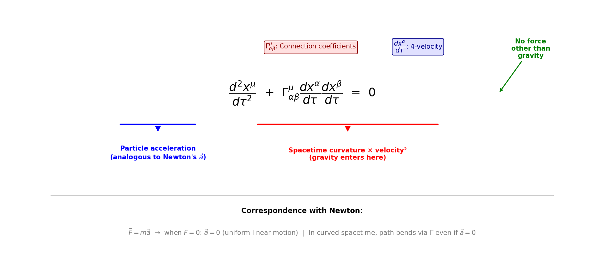
Fig. 2.5: The role of each term in the geodesic equation. The first term is the particle's acceleration (corresponding to Newton's \(\vec{a}\)), the second term is the effect of spacetime geometry on the particle's motion (gravity is absorbed here), and the right-hand side being zero means no forces other than gravity are present.
Also, notice that in the second term, \(\alpha\) and \(\beta\) appear both upstairs and downstairs? Specifically, in \(\Gamma^\mu_{\alpha\beta}\), \(\alpha\) is downstairs, while in \(\frac{dx^\alpha}{d\tau}\), \(\alpha\) is upstairs.
🔵 Kai: Wait. Isn't \(x^\alpha\) the "\(\alpha\)-th power of \(x\)"?
🟡 Lina: Good question. In high school, \(x^2\) means "\(x\) squared," but in relativity the convention is to write the component label as a superscript. So \(x^2\) means "the second component of the coordinate (the \(y\) direction)." It's confusing with exponentiation, but you distinguish by context — if the superscript in a relativity equation is a Greek letter like \(\mu, \nu, \alpha, \beta\), it's almost certainly a component label. Even when it's a number, within tensor equations it's read as a component label.
🔵 Kai: I'll probably be confused until I get used to it, but understood. Also, what's the difference between having an index upstairs versus downstairs?
🟡 Lina: At this stage, just think of it as "upstairs indices and downstairs indices follow different transformation rules under coordinate changes." Upper indices are called contravariant and lower indices are called covariant, but their precise meaning is studied in Ch. 6. What's important here is the rule: whenever the same index appears once upstairs and once downstairs, sum over that index — this is called the Einstein summation convention. It means summing over all values \(\alpha = 0, 1, 2, 3\). Similarly for \(\beta\) — the lower index \(\beta\) in \(\Gamma^\mu_{\alpha\beta}\) and the upper index \(\beta\) in \(\frac{dx^\beta}{d\tau}\) are paired, so we also sum over \(\beta = 0, 1, 2, 3\). That gives a sum of \(4 \times 4 = 16\) terms. It's a notation that omits the summation symbol \(\sum\), and we'll use it throughout.
A simple example: if we write \(A^\alpha B_\alpha\), it means \(A^0 B_0 + A^1 B_1 + A^2 B_2 + A^3 B_3\). Think of it as the 4-dimensional version of the dot product \(\vec{A} \cdot \vec{B} = A_x B_x + A_y B_y + A_z B_z\) you learned in high school. Let me summarize in a figure (Fig. 2.6 "Image of the Einstein summation convention").
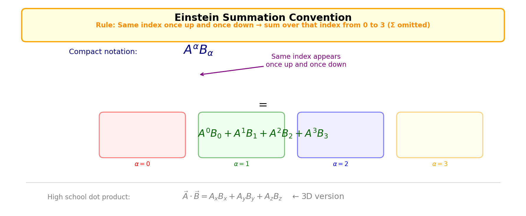
Fig. 2.6: Image of the Einstein summation convention. When the same index appears once upstairs and once downstairs, sum over that index from \(0\) to \(3\). This notation omits the \(\sum\) symbol and is used in all equations in relativity. {: #fig-gr-ch2-summation-convention } 🟡 Lina: And the right-hand side is zero — meaning no force. Compare with Newton's \(\vec{F} = m\vec{a}\). The "force" of gravity has disappeared from the right-hand side, and instead the \(\Gamma\) term has entered the left-hand side — the acceleration side. "Gravity is not a force but curvature of spacetime" is clearly visible in the mathematics too, isn't it?
⚪ Mei: I see. In Newton's formulation, gravity entered the right-hand side as a "force," but in Einstein's, it's absorbed into \(\Gamma\) on the left-hand side and the right-hand side becomes zero — the structure has completely changed.
🔵 Kai: What's the difference between a world line and a geodesic?
🟡 Lina: A world line is the general term for the trajectory any object traces on a spacetime diagram. Whether it's subject to forces or not, any object's trajectory is a world line. A geodesic is, among those, the world line of an object subject to no forces other than gravity — it's a special case of a world line.
🔵 Kai: "Other than gravity" — isn't gravity a force?
🟡 Lina: That's the decisive difference between Newton and Einstein (Fig. 2.7 "Comparison of Newton's and Einstein's views of gravity. Left").
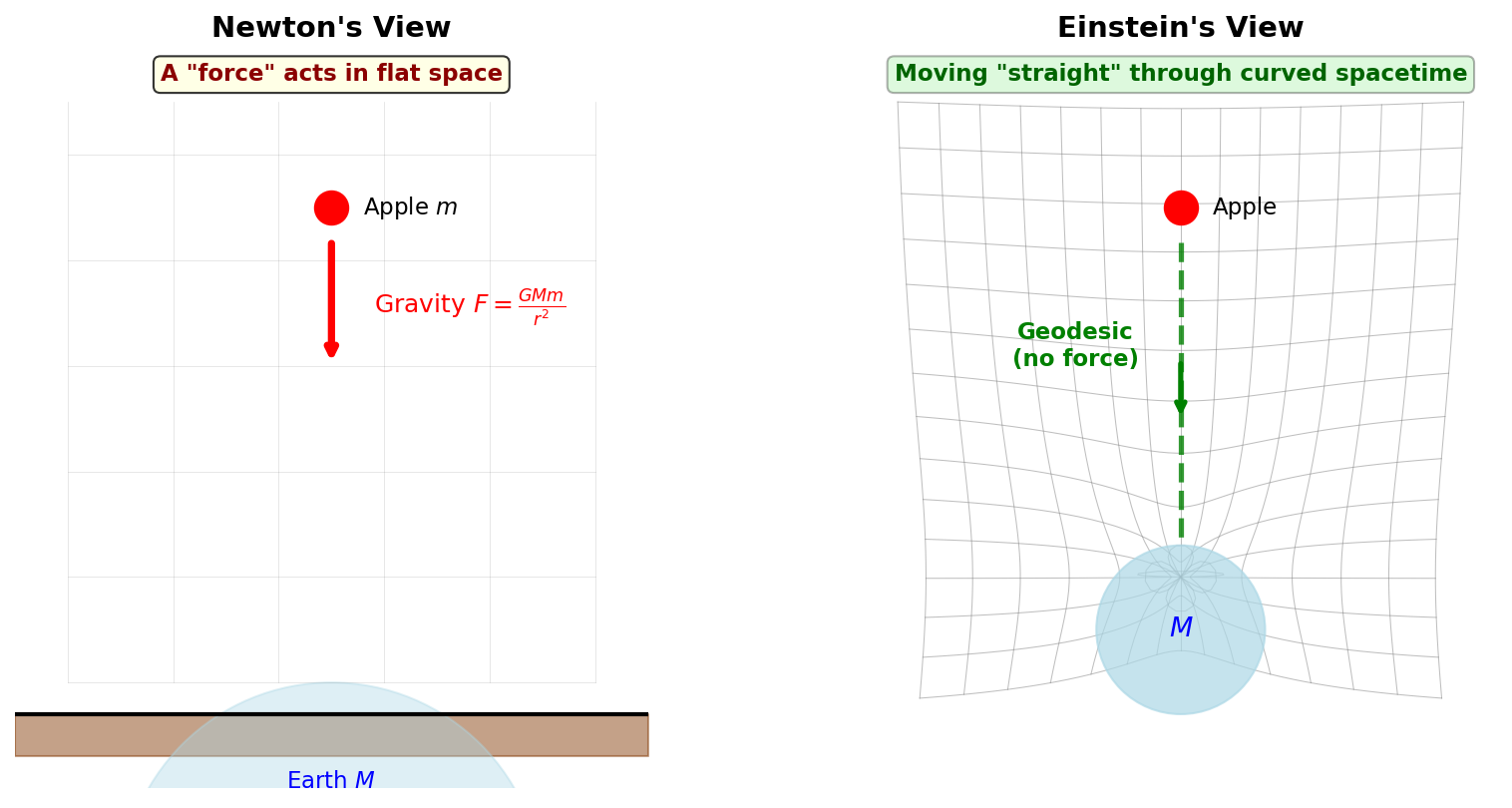
Fig. 2.7: Comparison of Newton's and Einstein's views of gravity. Left — Newton's view: In flat space, the apple falls because it's pulled by the "force" of gravity. Right — Einstein's view: The Earth's mass curves spacetime, and the apple simply travels "straight" along a geodesic in curved spacetime with no force acting on it.
- Newton's view: The apple falls because it's pulled by "the force of gravity"
- Einstein's view: The apple receives no force at all. It's simply going straight (along a geodesic) in curved spacetime
In Einstein's framework, gravity is absorbed into the curvature of spacetime rather than being a force. So it's not "only gravity is acting" but rather "no force other than gravity is acting = no force at all" — that's the meaning of a geodesic. The equation with zero on the right-hand side is specifically called the "geodesic equation" because "geodesic" is a geometric term meaning "extremal path in curved space." Let me draw the distinction between world lines and geodesics on a spacetime diagram (Fig. 2.8 "Difference between world lines and geodesics. Left").
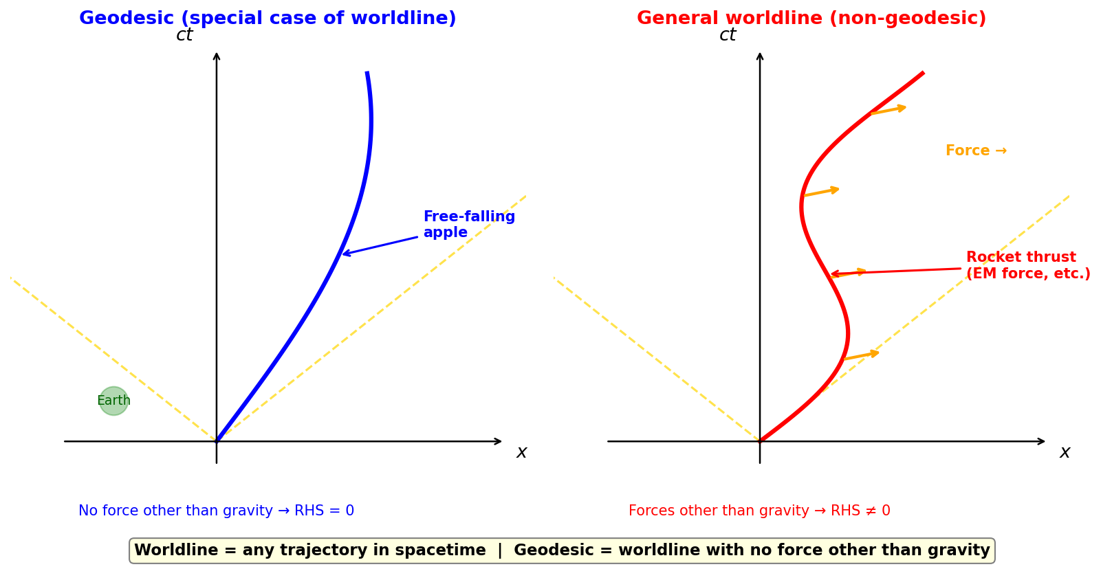
Fig. 2.8: Difference between world lines and geodesics. Left — Geodesic: the world line of an object receiving no force other than gravity (a freely falling apple). Right-hand side of the equation of motion = 0. Right — General world line (non-geodesic): the trajectory of an object receiving forces other than gravity, such as rocket thrust. Right-hand side ≠ 0.
✅ Comprehension Check: What is the difference between a world line and a geodesic?
Answer
A world line is the general term for the trajectory any object traces on a spacetime diagram — it's called a world line whether or not forces are acting. A geodesic is, among those, the world line of an object subject to no forces other than gravity — it's a special case of a world line.
🔵 Kai: So conversely, a charged particle being accelerated by electromagnetic force is not on a geodesic?
🟡 Lina: Exactly. Unlike gravity, electromagnetic force isn't absorbed into spacetime curvature, so it remains as a force.
🔵 Kai: What does the equation of motion look like in that case?
🟡 Lina: You just add "forces other than gravity" to the right-hand side of the geodesic equation. However, the geodesic equation as-is has the form "acceleration = 0" — if we're adding force to the right-hand side, we want the form "mass × acceleration = force." So we multiply the left-hand side by mass \(m\) and write force on the right-hand side. For example, adding the electromagnetic force (4-vector version of the Lorentz force) for a particle with charge \(q\) moving in an electromagnetic field:
Here \(\frac{dx^\nu}{d\tau}\) is the particle's 4-velocity (the 4-dimensional version of velocity that appeared earlier). You don't need to follow the details of the right-hand side now — what matters is the structure. \(F^{\mu}{}_{\nu}\) is a rank-2 tensor with one upper index \(\mu\) and one lower index \(\nu\). The indices are written with a space between them just to make clear that "the first is upper, the second is lower," but don't worry about this for now. And \(\nu\) appears once downstairs in \(F^{\mu}{}_{\nu}\) and once upstairs in \(\frac{dx^\nu}{d\tau}\), so it's contracted (summed over). Meanwhile, \(\mu\) appears only as an upper index on both sides — it doesn't form an "upper-and-lower pair," so it's not summed over. Such an index is called a free index.
🔵 Kai: Let me organize this. The contracted index \(\nu\) is summed over and disappears. The free index \(\mu\) remains, and choosing \(\mu = 0\) gives the time-direction equation, \(\mu = 1\) gives the \(x\)-direction... so this single line actually represents 4 equations simultaneously?
🟡 Lina: Exactly. One line for all four — that's the convenience of index notation. To summarize, there are two types of indices:
- Contracted indices (dummy indices): the same index appears once upstairs and once downstairs → sum over that index from \(0\) to \(3\) (the index disappears)
- Free indices: indices that don't form an upper-lower pair within each term. They appear in the same position (upper if upper) on both sides of the equation, and are not summed. They mean "the equation holds for whichever value \(\mu = 0, 1, 2, 3\) you choose," compactly writing 4 equations in one line
For example, choosing \(\mu = 1\) gives the \(x\)-direction equation, \(\mu = 2\) gives the \(y\)-direction equation, and so on. The \(F^{\mu}{}_{\nu}\) on the right-hand side is the electromagnetic field tensor — the 4-dimensional extension of the Lorentz force \(\vec{F} = q(\vec{E} + \vec{v} \times \vec{B})\) from high school. \(F^{\mu}{}_{\nu}\) is a rank-2 tensor with one contravariant (upper) index and one covariant (lower) index — the meaning of upper and lower indices is formally studied in Ch. 6, so don't worry about it now. The specific content is covered in Quantum Field Theory. By the way, \(\Gamma^\mu_{\alpha\beta}\) on the left-hand side also carries indices, but it's actually not a tensor — its transformation rule under coordinate changes differs from that of tensors. This distinction is studied in Ch. 8, so don't worry about it now.
Note on notation (preview): The meaning of the upper/lower indices of \(F^{\mu}{}_{\nu}\) is formally introduced in Ch. 6, so feel free to skip this for now.
The left-hand side is "acceleration in curved spacetime × mass" — gravity is absorbed into the \(\Gamma\) term. The right-hand side is the electromagnetic force. An equation with force on the right-hand side isn't called the "geodesic equation" but simply the "equation of motion." If a force bends the path, it's no longer a geodesic.
🔵 Kai: I see. If there's no force on the right-hand side, you can divide both sides by \(m\) and recover the original geodesic equation... ah, wait a moment. The fact that you can divide by \(m\) means mass \(m\) doesn't appear in the geodesic equation — does that mean objects with different masses trace the same trajectory? Is that saying the same thing as the experiment Galileo (legendarily) did at the Leaning Tower of Pisa?
🟡 Lina: Exactly. Galileo's "heavy and light objects fall the same way" is naturally incorporated in Einstein's framework as "all objects follow the same geodesic regardless of mass." This is the mathematical expression of the equality of inertial and gravitational mass (the equivalence principle). We'll look at it in detail in Ch. 5.
✅ Comprehension Check: The fact that the particle's mass \(m\) doesn't appear in the geodesic equation is connected to which physical principle?
Answer
It's connected to the equality of inertial and gravitational mass (the equivalence principle). Since mass doesn't appear in the equation, all objects follow the same geodesic regardless of mass.
🔵 Kai: By the way, who decides how the spacetime on the left-hand side curves?
🟡 Lina: That's determined by the Einstein equation — the goal ahead.
The left-hand side \(G_{\mu\nu}\) (Einstein tensor) represents the curvature of spacetime, and the right-hand side \(T_{\mu\nu}\) (energy-momentum tensor) represents the distribution of matter and energy. In other words, how matter and energy are distributed determines the curvature of spacetime — that's the answer to Kai's question. And since both sides are the same type of tensor (rank 2), this form holds in any coordinate system.
🔵 Kai: Matter determines the shape of spacetime, and the shape of spacetime determines how matter moves — they influence each other. ...But I have several questions. First, are the \(G_{\mu\nu}\) on the left and the \(G\) (gravitational constant) on the right related?
🟡 Lina: They're completely different things. \(G_{\mu\nu}\) is a tensor with indices (a quantity representing spacetime curvature), and \(G\) is just a constant with no indices (Newton's gravitational constant \(\approx 6.67 \times 10^{-11}\)). They happen to use the same letter of the alphabet, but they're physically unrelated. Distinguish them by context and the presence of indices.
🔵 Kai: Next, what's the "\(8\pi\)" in \(\frac{8\pi G}{c^4}\)? Why do \(8\) and the number \(\pi\) appear? And dividing by \(c^4\) is also puzzling.
🟡 Lina: That coefficient wasn't freely chosen by Einstein — it's determined by requiring consistency with Newton's Poisson equation \(\nabla^2 \Phi = 4\pi G\rho\). From the condition that the Einstein equation reduces to the Poisson equation in the limit of weak gravity and slow speeds, it must be \(8\pi G/c^4\). The origin of \(4\pi\) is, as we saw in Ch. 1, from the total solid angle \(4\pi\) steradians enclosing a sphere. The reason it becomes \(8\pi\) (\(4\pi\) times 2) comes from factors in the definition of the Einstein tensor \(G_{\mu\nu}\), but we can't derive it at this stage — we'll verify it by actual calculation in Ch. 14.
🔵 Kai: So it's determined by matching Newton's limit. Then what about \(c^4\)?
🟡 Lina: The \(c^4\) in the denominator is for matching dimensions. \(T_{\mu\nu}\) represents "energy or momentum per unit volume" and has dimensions of energy density — J/m³ (joules per cubic meter). Meanwhile, \(G_{\mu\nu}\) is constructed from second derivatives of the metric tensor and has dimensions of 1/m² (inverse length squared). Intuitively, recall from high school: if you differentiate \(y = f(x)\) where \(x\) is in meters and \(y\) is dimensionless, \(\frac{d^2 y}{dx^2}\) has units of \(1/\text{m}^2\). The metric tensor \(g_{\mu\nu}\) is (as we'll see in later chapters) dimensionless, and the coordinates \(x^\mu\) have dimensions of length. So differentiating \(g_{\mu\nu}\) twice with respect to coordinates gives dimensions of 1/m² — and \(G_{\mu\nu}\) is constructed from that, so it has the same dimensions (we'll rigorously check in Ch. 14). With the left-hand side in 1/m² and the right-hand side in J/m³, the dimensions don't match, so we need to insert constants between them to equalize the dimensions — \(G/c^4\) serves that role. The detailed dimensional check is done in Ch. 14, so for now just remember it as "the unique value that matches Newton's limit."
🔵 Kai: Also, the geodesic equation earlier also had \(\Gamma\), which represents "spacetime curvature." How is \(\Gamma\) different from \(G_{\mu\nu}\)?
🟡 Lina: Good question. In terms of physical causation, the order goes like this. Follow along with the flowchart (Fig. 2.9 "Basic structure of general relativity and relationships between quantities").
%%{init: {"theme": "default", "themeCSS": ".edgePath .path, .flowchart-link { stroke-width: 2px !important; }"}}%%
flowchart LR
    T["Matter & Energy<br/>T_μν"] -->|"Einstein equation"| g["Metric tensor<br/>g_μν"]
    g -->|"1st derivative"| Γ["Connection coefficients<br/>Γ^μ_αβ"]
    g -->|"2nd derivative"| R["Riemann tensor<br/>R^μ_ναβ"]
    Γ -->|"Geodesic equation"| orbit["Particle orbit"]
    R -->|"Contraction"| Ric["Ricci tensor<br/>R_μν"]
    Ric -->|"Further contraction"| G["Einstein tensor<br/>G_μν"]
Fig. 2.9: Basic structure of general relativity and relationships between quantities
First, the distribution of matter and energy \(T_{\mu\nu}\) is given. For example, a setup like "there exists a uniform spherical star of radius \(R\) and mass \(M\)" or "gas of density \(\rho\) is spread uniformly throughout the universe" is written mathematically in the form of \(T_{\mu\nu}\). It's the same idea as specifying the mass density \(\rho\) on the right-hand side of Newton's Poisson equation.
Next, solving the Einstein equation \(G_{\mu\nu} = \frac{8\pi G}{c^4}T_{\mu\nu}\) determines the metric tensor \(g_{\mu\nu}\) — that is, the shape of spacetime. The arrow from \(T_{\mu\nu}\) to \(g_{\mu\nu}\) in the flowchart represents this.
🔵 Kai: Wait a moment. The left-hand side of the equation is \(G_{\mu\nu}\), so why is it \(g_{\mu\nu}\) that gets determined?
🟡 Lina: \(G_{\mu\nu}\) (the Einstein tensor) is a quantity constructed from \(g_{\mu\nu}\) and its derivatives. So the Einstein equation is effectively a differential equation for \(g_{\mu\nu}\). It has the same structure as Newton's Poisson equation \(\nabla^2 \Phi = 4\pi G\rho\) being a differential equation for \(\Phi\).
Once \(g_{\mu\nu}\) is determined, differentiating it gives the connection coefficients \(\Gamma^\mu_{\alpha\beta}\). Finally, the geodesic equation determines the particle's orbit.
Here, both \(G_{\mu\nu}\) and \(\Gamma\) are constructed from \(g_{\mu\nu}\), but they involve different numbers of derivatives:
- First derivatives of \(g_{\mu\nu}\) → \(\Gamma^\mu_{\alpha\beta}\) (connection coefficients) → determines particle orbits via the geodesic equation
- Second derivatives of \(g_{\mu\nu}\) → Riemann tensor \(R^\mu{}_{\nu\alpha\beta}\) (the quantity that completely describes spacetime curvature, a rank-4 tensor with 4 indices) → contraction → Ricci tensor \(R_{\mu\nu}\) (rank-2 tensor) → further contraction → Ricci scalar \(R\) (rank-0 tensor) → combining \(R_{\mu\nu}\) and \(R\) gives \(G_{\mu\nu}\) (Einstein tensor) → determines the relationship with matter via the Einstein equation
🔵 Kai: In the flowchart there's an arrow going directly from \(g\) to \(R\), but there's also an arrow via \(\Gamma\). Which route does the actual calculation take?
🟡 Lina: The actual calculation always proceeds in the order \(g \to \Gamma \to R\) — first differentiate \(g\) once to get \(\Gamma\), then differentiate \(\Gamma\) further and combine with products of \(\Gamma\)'s to obtain \(R\). The arrow from \(g\) to \(R\) only shows the dependency relationship that "\(R\) is ultimately determined by second derivatives of \(g\)," not that you can skip \(\Gamma\). If it's confusing, just remember the single path \(g \to \Gamma \to R\). ...Now, the word "contraction" appeared in the flowchart.
🔵 Kai: Right, what is "contraction"?
🟡 Lina: Recall the Einstein summation convention we just learned. \(A^\alpha B_\alpha = A^0 B_0 + A^1 B_1 + A^2 B_2 + A^3 B_3\) — when we summed over the index \(\alpha\) matched upstairs and downstairs, \(\alpha\) disappeared and a scalar (no indices) remained, right?
🔵 Kai: Yes, like the dot product of two vectors.
🟡 Lina: Right. That was an example of matching indices between two vectors (rank-1 tensors), but the same idea can be applied within a single tensor — the operation of matching one pair of indices (one upper, one lower) within a tensor and summing is called contraction. For example, for a rank-2 tensor \(M^\mu{}_\nu\) (where \(M\) is anything — just a generic rank-2 tensor), matching \(\mu\) and \(\nu\) and summing gives \(M^0{}_0 + M^1{}_1 + M^2{}_2 + M^3{}_3\) — all indices disappear and a scalar remains.
🔵 Kai: Ah, it's like picking out and summing only the diagonal entries of a \(4 \times 4\) table?
🟡 Lina: Exactly. Viewing this in a \(4 \times 4\) table, it corresponds to picking out and summing only the entries along the diagonal from upper-left to lower-right. Writing it explicitly, when \(M^\mu{}_\nu\) is displayed as a table:
| \(\nu=0\) | \(\nu=1\) | \(\nu=2\) | \(\nu=3\) | |
|---|---|---|---|---|
| \(\mu=0\) | \(M^0{}_0\) | \(M^0{}_1\) | \(M^0{}_2\) | \(M^0{}_3\) |
| \(\mu=1\) | \(M^1{}_0\) | \(M^1{}_1\) | \(M^1{}_2\) | \(M^1{}_3\) |
| \(\mu=2\) | \(M^2{}_0\) | \(M^2{}_1\) | \(M^2{}_2\) | \(M^2{}_3\) |
| \(\mu=3\) | \(M^3{}_0\) | \(M^3{}_1\) | \(M^3{}_2\) | \(M^3{}_3\) |
Sum only the bold diagonal entries: \(M^0{}_0 + M^1{}_1 + M^2{}_2 + M^3{}_3\) (if you know matrices, think of it as the "trace"). However, this is the case of matching upper and lower indices within a single rank-2 tensor — the simplest example of contraction. More generally, you can also match indices between two tensors as in \(A^\alpha B_\alpha\), but the basic idea is the same — "sum over indices matched upper and lower, and those indices disappear." Each contraction eliminates one pair (two indices), so the rank decreases by two.
⚪ Mei: The rank drops by two with each contraction — it's an operation that compresses and summarizes information.
🔵 Kai: I understand that contraction lowers the rank. But with names like Riemann tensor, Ricci tensor all appearing at once, I'm getting confused... Do I have to memorize everything now?
🟡 Lina: For now, just grasping the names and "the flow of ranks decreasing" is sufficient. The specific content will be studied one by one in later chapters. Just stating the flow: contracting the Riemann tensor (4 indices, rank 4) once eliminates 2 indices to give the Ricci tensor (2 indices, rank 2). Contracting the Ricci tensor once more gives the Ricci scalar (no indices, rank 0). The Einstein tensor \(G_{\mu\nu}\) is constructed by combining the Ricci tensor and Ricci scalar — the flowchart simplifies this as "further contraction," but precisely it involves not just contraction but also a combination operation. The details are derived in Ch. 14. As a figure, the flow looks like this (Fig. 2.10 "Reduction of rank through tensor contraction").
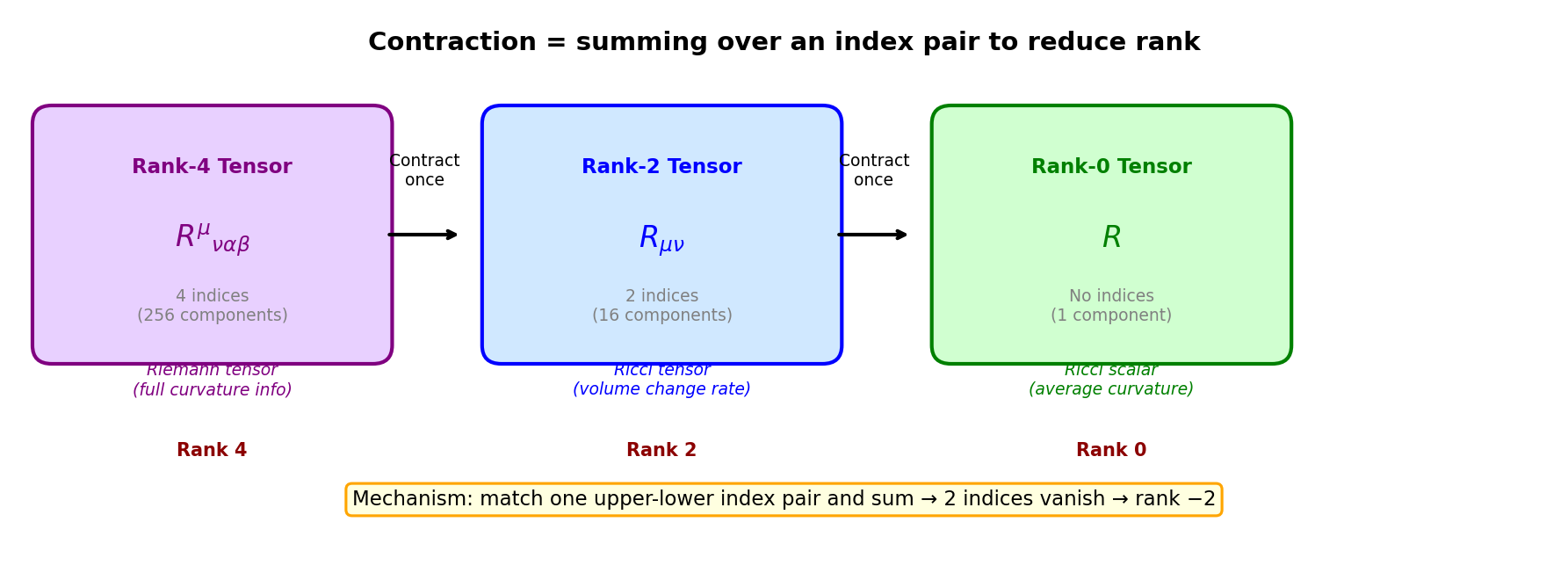
Fig. 2.10: Reduction of rank through tensor contraction. Contracting the rank-4 Riemann tensor (256 components) once gives the rank-2 Ricci tensor (16 components); contracting once more gives the rank-0 Ricci scalar (1 component). Each contraction eliminates 2 indices, compressing information.
The detailed calculations come in later chapters, so for now just think of it as "an operation that compresses information."
In other words, \(G_{\mu\nu}\) is a quantity constructed from derivatives and products of \(\Gamma\).
🔵 Kai: The upper route (\(\Gamma\) → orbit) alone determines the particle's motion, right? What's the lower route (Riemann → \(G_{\mu\nu}\)) used for?
🟡 Lina: It has two uses. First, it's used to determine \(g_{\mu\nu}\) itself. Look at the far left of the flowchart — the Einstein equation determines \(g_{\mu\nu}\) from the matter distribution \(T_{\mu\nu}\), and its left-hand side is \(G_{\mu\nu}\), right? So the lower route is a tool for "determining the shape of spacetime from how matter is distributed." Second, it's used to diagnose "how much a given spacetime is curved." For example, when the components of the metric behave strangely at a certain location near a black hole, to determine "is spacetime really breaking down, or is it just a bad choice of coordinates?" we need to examine invariants constructed from the Riemann tensor. We'll do this in detail in Ch. 16. For just finding particle orbits, the upper route suffices.
⚪ Mei: So the upper route determines "how a particle moves in spacetime," and the lower route is for "determining the shape of spacetime itself" and "examining the degree of curvature" — but both start from the same metric tensor \(g_{\mu\nu}\).
🔵 Kai: Looking at the flowchart, everything starts from \(g_{\mu\nu}\). The metric tensor really is the protagonist. ...But if matter \(T_{\mu\nu}\) curves spacetime and curved spacetime determines how matter moves, they're influencing each other — doesn't that go in circles? How do you solve it?
✅ Comprehension Check: What does it physically mean that the right-hand side of the geodesic equation is zero?
Answer
It means no forces (other than gravity) are acting on the particle. Gravity is not a force but is absorbed into the \(\Gamma\) term on the left-hand side as spacetime curvature, so it doesn't appear on the right-hand side.
✅ Comprehension Check: In the Einstein equation \(G_{\mu\nu} = \frac{8\pi G}{c^4}T_{\mu\nu}\), what do the left-hand side and right-hand side represent respectively?
Answer
The left-hand side \(G_{\mu\nu}\) (Einstein tensor) represents the curvature of spacetime, and the right-hand side \(T_{\mu\nu}\) (energy-momentum tensor) represents the distribution of matter and energy. The relationship is "how matter is distributed determines the curvature of spacetime."
📝 Exercises:
- Correspondence between Newton's and Einstein's two pillars → Problem B-3. The Two Pillars Correspondence between Newton and Einstein, Understanding the geodesic equation → Problem M-1. Understanding the Geodesic Equation, Coefficient of the Einstein equation → Problem M-2. Coefficient of the Einstein Equation, Quantities derived from the metric tensor → Problem A-1. Quantities Derived from the Metric Tensor
🟡 Lina: Let's compare the Newton and Einstein frameworks side by side.
Table 2.3: Correspondence between Newtonian mechanics and general relativity
| Newton | Einstein (General Relativity) | |
|---|---|---|
| Particle motion | \(\vec{F} = m\vec{a}\) (equation of motion) | \(\frac{d^2 x^\mu}{d\tau^2} + \Gamma^\mu_{\alpha\beta}\frac{dx^\alpha}{d\tau}\frac{dx^\beta}{d\tau} = 0\) (geodesic equation; add to the right-hand side if forces other than gravity are present) |
| Field equation | \(\nabla^2 \Phi = 4\pi G\rho\) (Poisson equation) | \(G_{\mu\nu} = \frac{8\pi G}{c^4}T_{\mu\nu}\) (Einstein equation) |
| Nature of gravity | Force \(F = -GMm/r^2\) | Curvature of spacetime |
| Protagonist | Gravitational potential \(\Phi\) (scalar) | Metric tensor \(g_{\mu\nu}\) (rank-2 tensor) |
⚪ Mei: They correspond one-to-one beautifully. A scalar becomes a rank-2 tensor, density becomes the energy-momentum tensor — the rank goes up but the structure is the same, which makes it easy to understand.
🟡 Lina: Newton also had a "field equation" — the Poisson equation that determines the gravitational potential \(\Phi\).
The Einstein equation
is its generalization, where the scalar \(\Phi\) is replaced by the rank-2 tensor \(g_{\mu\nu}\), and the density \(\rho\) is replaced by the energy-momentum tensor \(T_{\mu\nu}\). Indeed, in the limit of weak gravity and slow speeds, the Einstein equation reduces to the Poisson equation.
🔵 Kai: So Newton's theory is an approximation of Einstein's theory.
🟡 Lina: Exactly. That's why in Einstein's framework, rank-1 tensors (vectors) alone aren't sufficient — we need rank-2 tensors.
✅ Comprehension Check: When transitioning from Newton's theory of gravity to Einstein's general relativity, what does the main physical quantity change from the scalar \(\Phi\) to? And what is the rank of that tensor?
Answer
It changes from the gravitational potential \(\Phi\) (rank-0 tensor = scalar) to the metric tensor \(g_{\mu\nu}\) (rank-2 tensor). Similarly, the right-hand side of the field equation is also extended from the density \(\rho\) (scalar) to the energy-momentum tensor \(T_{\mu\nu}\) (rank-2 tensor).
2.4 The Journey Ahead — Starting from Rank-0 Tensors
🔵 Kai: Matter and energy determine the shape of spacetime through the Einstein equation, and particles move along geodesics in that spacetime — what a grand framework. But we still don't know the content of the metric tensor \(g_{\mu\nu}\) or the Riemann tensor at all. Where do we start?
🟡 Lina: Good question. Let's confirm the path of building up from tensor rank 0 step by step in a figure (Fig. 2.11 "Roadmap of the journey ahead. Rank-0 tensor (spacetime interval \(ds^2\)) → Rank-1 tensor (4-vectors) → Rank-2 tensor (metric \(g_{\mu\nu}\)) → Einstein equation").
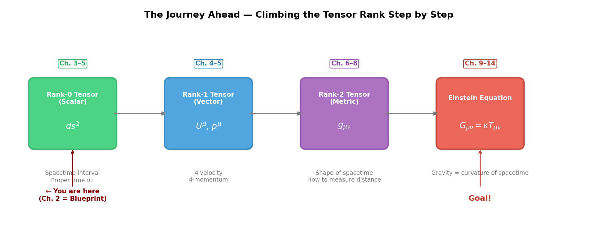
Fig. 2.11: Roadmap of the journey ahead. Rank-0 tensor (spacetime interval \(ds^2\)) → Rank-1 tensor (4-vectors) → Rank-2 tensor (metric \(g_{\mu\nu}\)) → Einstein equation — building up step by step, increasing the tensor rank one level at a time.
🟡 Lina: So the first piece of this journey starts with the simplest tensor — a rank-0 tensor (scalar) — that is, an invariant. As we saw in 2.1 "Scalars, Vectors, and Tensors", the representative example of an invariant in 3-dimensional space was the distance between two points. When we extend this to 4-dimensional spacetime, what form does the invariant take? Showing just the conclusion first,
The fact that this \(ds^2\) is "an invariant that gives the same value regardless of which inertial frame you calculate it from" — that is, that it's a rank-0 tensor — will be proven from the principle of the constancy of the speed of light in the next Ch. 3. For now, just look at the form.
🔵 Kai: The spatial part \(dx^2 + dy^2 + dz^2\) looks like the Pythagorean theorem, but the time term \(-(cdt)^2\) has a minus sign — that's strange.
🟡 Lina: Here \((cdt)^2 = (c \times dt)^2 = c^2 \cdot dt^2\) (the square of "\(c\) times \(dt\)" as a whole), and \(dx^2\) means \((dx)^2\) (the square of \(dx\)) — note it's not \(d(x^2)\). The same reading applies to \(dy^2\), \(dz^2\), and \((cdt)^2\). By the way, the \(x, y, z\) here are the spatial coordinates themselves (position in the \(x\) direction, \(y\) direction, \(z\) direction), distinct from the "superscript numbers" in the component labels \(x^1, x^2, x^3\) mentioned earlier — it's confusing, but the \(ds^2\) formula is traditionally written this way. \(dt\), \(dx\), \(dy\), \(dz\) are infinitesimal changes in time and space respectively. In high school, you wrote the square of the distance between two points using \(\Delta x\), \(\Delta y\), \(\Delta z\) with the Pythagorean theorem \(\Delta x^2 + \Delta y^2 + \Delta z^2\). \(\Delta x\) meant "the change in \(x\)." Taking this \(\Delta x\) to the infinitesimally small limit gives \(dx\) — the same symbol as the \(dx\) in \(\frac{dy}{dx}\) from high school, meaning "an infinitesimally small change." The same goes for \(dy\), \(dz\), \(dt\). \(ds^2\) represents "the square of the interval between two infinitesimally close points in spacetime." Think of it as extending the formula for the square of the distance between two points in 3-dimensional space, \(dx^2 + dy^2 + dz^2\) (the infinitesimal version of the Pythagorean theorem), to include the time direction. The speed of light \(c\) multiplies \(dt\) for the same reason we saw in the spacetime diagram — to convert time to length dimensions (\(c \times dt\) is "the distance light travels during \(dt\)").
🔵 Kai: The spatial terms are all positive, but the time term has a minus sign. Why is only time negative? Also, this means \(ds^2\) can be negative, right? Isn't it strange for the square of a distance to be negative?
🟡 Lina: Good questions. \(ds^2\) is not "the square of a distance" in the ordinary sense — since it's an "interval in spacetime" combining time and space, it can be positive, negative, or zero. The complete answer to why the minus sign is needed comes in the next Ch. 3 where we derive it from the principle of the constancy of the speed of light, but let me give the intuition first: light travels a distance \(c \times dt\) during time \(dt\), so \(dx = c\,dt\), giving \(-(cdt)^2 + dx^2 = 0\).
⚪ Mei: The fact that \(ds^2 = 0\) for light is because the negative and positive terms exactly cancel.
🟡 Lina: Right. A particle slower than light can only travel a shorter distance than light in the same coordinate time \(dt\). That is, the square of the distance traveled by the particle \(dx^2+dy^2+dz^2\) is less than the square of the distance traveled by light \((cdt)^2\) — \(dx^2+dy^2+dz^2 < (cdt)^2\) (regardless of direction, the sum in all 3 directions cannot exceed light's distance). Substituting into the formula, \(ds^2 = -(cdt)^2 + (dx^2+dy^2+dz^2)\), and since \((cdt)^2 > dx^2+dy^2+dz^2\), the negative term wins, making the whole thing \(ds^2 < 0\).
🔵 Kai: I see — for light \(ds^2 = 0\), and for anything slower than light \(ds^2 < 0\). But I understand the fundamental reason why time must have a minus sign will become clear in the next chapter. Even so, \(ds^2\) being negative — "a square being negative" — feels very uncomfortable...
🟡 Lina: That uncomfortable feeling is a correct instinct. Actually, it's better to think of \(ds^2\) not as "the square of something" but as a single quantity named "\(ds^2\)" as a whole. The square of an ordinary distance is always positive, but a spacetime "interval" is a quantity mixing time and space, so it can be positive, negative, or zero — that's why we call it an "interval" rather than a "distance."
Note on sign convention: Some textbooks use \(ds^2 = +(cdt)^2 - dx^2 - dy^2 - dz^2\), with plus for time and minus for space. This book adopts \(ds^2 = -(cdt)^2 + dx^2 + dy^2 + dz^2\) (minus for time, plus for space). Both conventions give the same physical conclusions, but the meaning of the sign of \(ds^2\) is reversed, so be careful when consulting other textbooks.
⚪ Mei: So the sign of \(ds^2\) tells us "faster or slower than light."
🟡 Lina: Exactly. By the way, previewing the relationship with the metric tensor \(g_{\mu\nu}\) that appeared earlier: the coefficients in this formula (time direction is \(-1\), spatial directions are \(+1, +1, +1\)) correspond precisely to the components of \(g_{\mu\nu}\) — I'll formally introduce this in Ch. 6. Let me draw a figure comparing spatial distance and spacetime interval (Fig. 2.12 "Comparison of Euclidean geometry and Minkowski geometry. Left").
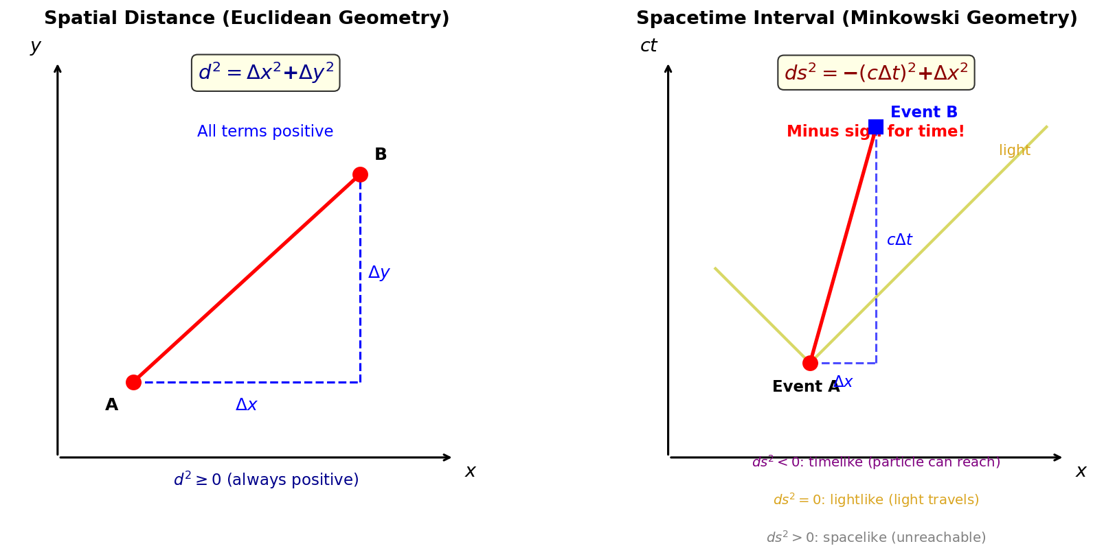
Fig. 2.12: Comparison of Euclidean geometry and Minkowski geometry. Left — In ordinary space, the square of the distance is \(\Delta x^2 + \Delta y^2\), always positive. Right — The spacetime interval is \(ds^2 = -(c\Delta t)^2 + \Delta x^2\), with a minus sign on the time term, so it can be positive, negative, or zero. \(ds^2 < 0\) (timelike) means reachable by a massive particle, \(ds^2 = 0\) (lightlike) means the path light takes, \(ds^2 > 0\) (spacelike) means an unreachable relationship.
🟡 Lina: As shown in the figure, \(ds^2 < 0\) corresponds to a relationship reachable by massive particles (timelike), \(ds^2 = 0\) corresponds to paths light takes (lightlike), and \(ds^2 > 0\) corresponds to relationships unreachable even by light (spacelike). Why the minus sign is needed, and what each case physically means — deriving this step by step from the principle of the constancy of the speed of light is the core of the next Ch. 3. For now, just remember that "\(ds^2\) being negative is physically meaningful — in fact, for massive particles \(ds^2 < 0\) is the norm."
⚪ Mei: The sign of \(ds^2\) tells us "reachable by a massive particle, passable only by light, or unreachable by either." I'm looking forward to starting from this rank-0 tensor in the next chapter.
🟡 Lina: Since many symbols appeared in this chapter, let me summarize them at the end.
Table 2.4: Summary of main symbols introduced in this chapter
| Symbol | Pronunciation | Meaning | Chapter where studied in detail |
|---|---|---|---|
| \(\mu, \nu, \alpha, \beta\) | mu, nu, alpha, beta | Spacetime indices (0, 1, 2, 3) | Chapter 4 |
| \(\tau\) | tau | Proper time (time ticked by the particle's clock) | Chapter 3 |
| \(ds^2\) | dee-ess-squared | Spacetime interval (rank-0 tensor) | Chapter 3 |
| \(g_{\mu\nu}\) | gee-mu-nu | Metric tensor (rank-2 tensor determining the shape of spacetime) | Chapter 6 |
| \(\Gamma^\mu_{\alpha\beta}\) | gamma | Connection coefficients (determined from first derivatives of the metric) | Chapter 8 |
| \(R^\mu{}_{\nu\alpha\beta}\) | Riemann tensor | Riemann tensor (complete information about spacetime curvature) | Chapter 9 |
| \(R_{\mu\nu}\) | Ricci tensor | Ricci tensor (contraction of Riemann) | Chapter 10 |
| \(G_{\mu\nu}\) | Einstein tensor | Einstein tensor (left-hand side of the Einstein equation) | Chapter 14 |
| \(T_{\mu\nu}\) | tee-mu-nu | Energy-momentum tensor (distribution of matter) | Chapter 14 |
Preview of the Next Chapter
In Ch. 3 title, we concretely construct the first piece of this blueprint. Starting from Einstein's two postulates — the principle of relativity and the constancy of the speed of light — we derive the most fundamental rank-0 tensor (invariant) — the spacetime interval \(ds^2\) — and from there construct the Lorentz transformation, time dilation, and the Minkowski metric all at once.
References
- Schutz, B. F. A First Course in General Relativity, 3rd ed., Chapter 1. Cambridge University Press, 2022.
- Lancaster, T. and Blundell, S. J. General Relativity for the Gifted Amateur, Chapter 1. Oxford University Press, 2014.
- Carroll, S. M. Spacetime and Geometry: An Introduction to General Relativity, Chapter 1. Addison-Wesley, 2004.
Feedback on this page
Let us know if something was unclear, incorrect, or could be improved.