Appendix A Solutions
← Back to problems | Back to chapter
Table of Contents
Basic
- B-1. Component Calculation of the Cross Product
- B-2. Orthogonality of the Cross Product
- B-3. Scalar Triple Product
- B-4. Gradient of a Scalar Field
- B-5. Divergence of a Vector Field
- B-6. Curl of a Vector Field
- B-7. Laplacian of a Scalar Field
- B-8. Verification of the Lagrange Identity
- B-9. Verification of the BAC-CAB Formula
- B-10. Verifying rot(grad) = 0
Medium
- M-1. Proof of the BAC-CAB Formula
- M-2. Proof that div(curl) = 0
- M-3. Inner Product of Two Cross Products Formula
- M-4. Product Rule for Divergence
- M-5. Gauss's Theorem and the Coulomb Electric Field
Advanced
Basic
B-1. Component Calculation of the Cross Product
Problem:
Calculate the cross product \(\boldsymbol{a} \times \boldsymbol{b}\) of vectors \(\boldsymbol{a} = (2,\, 1,\, -1)\) and \(\boldsymbol{b} = (0,\, 3,\, 2)\) component by component according to the definition.
Solution strategy: Expand the formal determinant by cofactors along the first row.
Calculation:
Verification: By the anticommutativity property, \(\boldsymbol{b} \times \boldsymbol{a} = (-5, 4, -6)\) should hold. Indeed, \((\boldsymbol{b} \times \boldsymbol{a})_x = 3 \cdot (-1) - 2 \cdot 1 = -5\) ✓
B-2. Orthogonality of the Cross Product
Problem:
Verify that \(\boldsymbol{a} \times \boldsymbol{b}\) obtained in Problem A.1 is orthogonal to \(\boldsymbol{a}\) by computing the dot product \((\boldsymbol{a} \times \boldsymbol{b}) \cdot \boldsymbol{a}\).
Calculation:
Verification: Checking the dot product with \(\boldsymbol{b}\) as well: \(5 \cdot 0 + (-4) \cdot 3 + 6 \cdot 2 = 0 - 12 + 12 = 0\) ✓
B-3. Scalar Triple Product
Problem:
Calculate the scalar triple product \(\boldsymbol{a} \cdot (\boldsymbol{b} \times \boldsymbol{c})\) of the vectors \(\boldsymbol{a} = (1,\, 0,\, 2)\), \(\boldsymbol{b} = (3,\, 1,\, 0)\), \(\boldsymbol{c} = (0,\, -1,\, 1)\) as a \(3 \times 3\) determinant.
Calculation:
Cofactor expansion along the first row:
Verification (Sarrus' method):
Sum of downward-right diagonals: \(a_{11}a_{22}a_{33} + a_{12}a_{23}a_{31} + a_{13}a_{21}a_{32} = 1 \cdot 1 \cdot 1 + 0 \cdot 0 \cdot 0 + 2 \cdot 3 \cdot (-1) = 1 + 0 - 6 = -5\)
Sum of downward-left diagonals: \(a_{13}a_{22}a_{31} + a_{12}a_{21}a_{33} + a_{11}a_{23}a_{32} = 2 \cdot 1 \cdot 0 + 0 \cdot 3 \cdot 1 + 1 \cdot 0 \cdot (-1) = 0 + 0 + 0 = 0\)
Determinant \(= -5 - 0 = -5\) ✓
B-4. Gradient of a Scalar Field
Problem:
Find the gradient \(\nabla\varphi\) of the scalar field \(\varphi(x, y, z) = x^2 y + y^2 z + z^2 x\).
Calculation:
Verification: Check the dimensions (partial derivatives of each monomial in \(\varphi\) with respect to each variable). \(\partial(x^2 y)/\partial x = 2xy\) ✓, \(\partial(y^2 z)/\partial x = 0\) ✓, \(\partial(z^2 x)/\partial x = z^2\) ✓. The other components follow similarly.
B-5. Divergence of a Vector Field
Problem:
Reference Figure: Figure A.1: Cross Product (Appendix A)
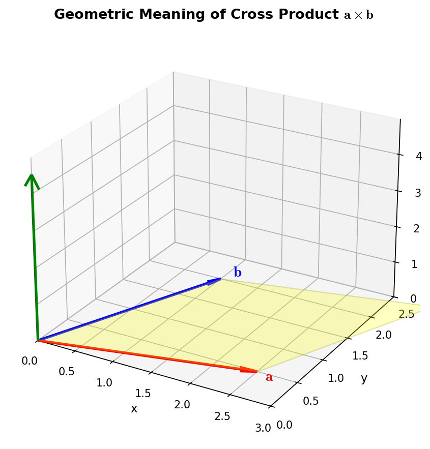
Calculate the divergence \(\nabla \cdot \boldsymbol{F}\) of the vector field \(\boldsymbol{F} = (x^2 y,\; y^2 z,\; z^2 x)\).
Calculation:
Verification: Checking each partial derivative individually. \(\partial(x^2 y)/\partial x = 2xy\) (treating \(y\) as a constant) ✓
B-6. Curl of a Vector Field
Problem:
Reference Figure: Figure A.1: Geometry of the Cross Product (Appendix A)
Compute the curl \(\nabla \times \boldsymbol{F}\) of the vector field \(\boldsymbol{F} = (yz,\; xz,\; xy)\) component by component.
Calculation:
Verification: Since \(\boldsymbol{F} = (yz, xz, xy) = \nabla(xyz)\), the curl of a gradient field is identically zero. Indeed, \(\partial(xyz)/\partial x = yz\), \(\partial(xyz)/\partial y = xz\), \(\partial(xyz)/\partial z = xy\) ✓
B-7. Laplacian of a Scalar Field
Problem:
Compute the Laplacian \(\Delta\varphi = \nabla^2\varphi\) of the scalar field \(\varphi = e^x \sin y + z^3\).
Calculation:
Verification: The \(e^x \sin y\) part is a two-dimensional harmonic function (\(\Delta_{2D}(e^x \sin y) = 0\)), so its contribution to the Laplacian is zero. The Laplacian of \(z^3\) is \(6z\). Consistent ✓
B-8. Verification of the Lagrange Identity
Problem:
Using the Lagrange identity, compute \(|\boldsymbol{a} \times \boldsymbol{b}|^2\) as \(|\boldsymbol{a}|^2|\boldsymbol{b}|^2 - (\boldsymbol{a} \cdot \boldsymbol{b})^2\) for \(\boldsymbol{a} = (1,\, 2,\, 0)\) and \(\boldsymbol{b} = (0,\, 1,\, 3)\), and verify that the result agrees with the square of the magnitude of the cross product computed directly.
Calculation (right-hand side):
Calculation (left-hand side):
Both sides agree ✓
B-9. Verification of the BAC-CAB Formula
Problem:
Verify the BAC-CAB formula \(\boldsymbol{a} \times (\boldsymbol{b} \times \boldsymbol{c}) = \boldsymbol{b}(\boldsymbol{a} \cdot \boldsymbol{c}) - \boldsymbol{c}(\boldsymbol{a} \cdot \boldsymbol{b})\) by computing the left-hand side and the right-hand side separately for \(\boldsymbol{a} = (1,0,0)\), \(\boldsymbol{b} = (0,1,0)\), \(\boldsymbol{c} = (0,0,1)\), and confirm that they are equal.
Calculating the left-hand side:
Calculating the right-hand side:
Verification: Since \(\boldsymbol{a} = \boldsymbol{e}_1\), \(\boldsymbol{b} = \boldsymbol{e}_2\), \(\boldsymbol{c} = \boldsymbol{e}_3\) are mutually orthogonal standard basis vectors, \(\boldsymbol{a} \cdot \boldsymbol{b} = \boldsymbol{a} \cdot \boldsymbol{c} = 0\) is natural. Also, since \(\boldsymbol{b} \times \boldsymbol{c} = \boldsymbol{e}_1 = \boldsymbol{a}\), the result \(\boldsymbol{a} \times \boldsymbol{a} = \boldsymbol{0}\) is also natural ✓
B-10. Verifying rot(grad) = 0
Problem:
Reference: The rotation identity \(\nabla \times (\nabla\varphi) = 0\) is explained in Section A.5 of Appendix A.
For the scalar field \(\varphi(x, y, z) = x^2 + y^2 + z^2\), verify by component calculation that \(\operatorname{rot}(\operatorname{grad}\varphi) = \boldsymbol{0}\) holds.
Calculation:
Let \(\boldsymbol{G} = \nabla\varphi = (2x, 2y, 2z)\):
Verification: This is a concrete example of the identity \(\operatorname{curl}(\operatorname{grad}\varphi) = \boldsymbol{0}\). Each component automatically vanishes due to the symmetry of mixed partial derivatives (since \(\varphi\) is of class \(C^2\)), e.g., \(\frac{\partial^2 \varphi}{\partial y \partial z} - \frac{\partial^2 \varphi}{\partial z \partial y} = 0\) ✓
Medium
M-1. Proof of the BAC-CAB Formula
Problem:
Prove that
by expanding the \(x\)-components of both sides in terms of the general components \(a_i, b_i, c_i\) and comparing them. Explain (using a symmetry argument) why the same identity holds for the \(y\) and \(z\) components as well.
Solution Strategy:
Expand the \(x\) component of the left-hand side \(\boldsymbol{a} \times (\boldsymbol{b} \times \boldsymbol{c})\) by applying the definition of the cross product twice. Also expand the \(x\) component of the right-hand side \(\boldsymbol{b}(\boldsymbol{a} \cdot \boldsymbol{c}) - \boldsymbol{c}(\boldsymbol{a} \cdot \boldsymbol{b})\), and show that both are equal.
Detailed Calculation:
\(x\) component of the left-hand side:
First, write out the components of \(\boldsymbol{b} \times \boldsymbol{c}\):
The \(x\) component of \(\boldsymbol{a} \times (\boldsymbol{b} \times \boldsymbol{c})\) is:
Now add and subtract \(a_1 c_1\) and \(a_1 b_1\) (since \(b_1 a_1 c_1 - c_1 a_1 b_1 = 0\), the value is unchanged):
\(x\) component of the right-hand side:
Final Answer:
The \(x\) components of the left-hand side and right-hand side are equal:
Regarding the \(y\) and \(z\) components: The calculation above uses only the cyclic structure of the indices \(1, 2, 3\). Since the definition of the cross product has the same form under cyclic permutations of the indices \((1 \to 2 \to 3 \to 1)\), the proof for the \(y\) component is obtained by replacing \(1 \to 2\), \(2 \to 3\), \(3 \to 1\) in the \(x\) component proof, and the proof for the \(z\) component is obtained by replacing \(1 \to 3\), \(2 \to 1\), \(3 \to 2\).
Therefore, the equality holds for all three components, and the BAC-CAB formula is proved. \(\blacksquare\)
Verification:
Confirmed with a specific numerical example (standard basis vectors) in D9 ✓
M-2. Proof that div(curl) = 0
Problem:
Reference: The divergence identity \(\nabla \cdot (\nabla \times \mathbf{F}) = 0\) is discussed in Section A.5 of Appendix A.
Prove that this holds using component representation. Also, briefly explain how this identity is related to the physical fact that "magnetic monopoles do not exist" (\(\operatorname{div}\boldsymbol{B} = 0\) and \(\boldsymbol{B} = \operatorname{rot}\boldsymbol{A}\)).
Solution Strategy:
Write out each component of \(\operatorname{rot}\boldsymbol{F}\), then take the \(\operatorname{div}\). By exchanging the order of partial derivatives, all terms pair up and cancel.
Detailed Calculation:
Let \(\boldsymbol{F} = (F_1, F_2, F_3)\). The components of the curl are:
Taking the divergence:
If \(\boldsymbol{F}\) is sufficiently smooth (class \(C^2\)), the order of partial differentiation is interchangeable: \(\frac{\partial^2 F_i}{\partial x_j \partial x_k} = \frac{\partial^2 F_i}{\partial x_k \partial x_j}\). Therefore:
- \(\frac{\partial^2 F_3}{\partial x \partial y}\) and \(-\frac{\partial^2 F_3}{\partial y \partial x}\) cancel
- \(-\frac{\partial^2 F_2}{\partial x \partial z}\) and \(\frac{\partial^2 F_2}{\partial z \partial x}\) cancel
- \(\frac{\partial^2 F_1}{\partial y \partial z}\) and \(-\frac{\partial^2 F_1}{\partial z \partial y}\) cancel
Physical Meaning:
In electromagnetism, the magnetic field \(\boldsymbol{B}\) can be written using a vector potential \(\boldsymbol{A}\) as \(\boldsymbol{B} = \nabla \times \boldsymbol{A}\). Applying the identity above:
This corresponds to one of Maxwell's equations, \(\nabla \cdot \boldsymbol{B} = 0\) (the non-existence of magnetic monopoles). In other words, the fact that the magnetic field can be expressed as the curl of a vector potential is automatically consistent with the non-existence of magnetic monopoles, by virtue of the mathematical identity \(\operatorname{div}(\operatorname{rot}) = 0\). Conversely, if magnetic monopoles were to exist, then \(\nabla \cdot \boldsymbol{B} \neq 0\), and \(\boldsymbol{B}\) could no longer be globally expressed as the curl of a single vector potential. \(\blacksquare\)
M-3. Inner Product of Two Cross Products Formula
Problem:
By substituting \(\boldsymbol{c} = \boldsymbol{a}\) and \(\boldsymbol{d} = \boldsymbol{b}\) into
derive the Lagrange identity
Furthermore, using this result, show that \(|\boldsymbol{a} \times \boldsymbol{b}| = |\boldsymbol{a}||\boldsymbol{b}|\sin\theta\) (where \(\theta\) is the angle between \(\boldsymbol{a}\) and \(\boldsymbol{b}\)).
Detailed Calculation:
Derivation of the Lagrange identity:
The formula for the inner product of two cross products:
Substituting \(\boldsymbol{c} = \boldsymbol{a}\), \(\boldsymbol{d} = \boldsymbol{b}\):
Derivation of \(|\boldsymbol{a} \times \boldsymbol{b}| = |\boldsymbol{a}||\boldsymbol{b}|\sin\theta\):
Let \(\theta\) (\(0 \leq \theta \leq \pi\)) be the angle between \(\boldsymbol{a}\) and \(\boldsymbol{b}\). Since \(\boldsymbol{a} \cdot \boldsymbol{b} = |\boldsymbol{a}||\boldsymbol{b}|\cos\theta\):
Since \(\sin\theta \geq 0\) for \(0 \leq \theta \leq \pi\), taking the positive square root of both sides:
Verification:
When \(\theta = 0\) (parallel): \(|\boldsymbol{a} \times \boldsymbol{b}| = 0\) ✓ (the cross product of parallel vectors is zero)
When \(\theta = \pi/2\) (orthogonal): \(|\boldsymbol{a} \times \boldsymbol{b}| = |\boldsymbol{a}||\boldsymbol{b}|\) ✓ (for example, \(\boldsymbol{e}_1 \times \boldsymbol{e}_2 = \boldsymbol{e}_3\) with \(|\boldsymbol{e}_3| = 1 = 1 \cdot 1\))
When \(\theta = \pi\) (antiparallel): \(|\boldsymbol{a} \times \boldsymbol{b}| = 0\) ✓ (\(\sin\pi = 0\), and the cross product of antiparallel vectors is also zero)
Also confirmed with the numerical example from D8 ✓
M-4. Product Rule for Divergence
Problem:
Reference: For product rule identities, see the list of identities in A.5 of Appendix A.
Prove the following identity using component notation:
Solution Strategy:
Write \(\operatorname{div}(\varphi\,\boldsymbol{F})\) in component form and apply the Leibniz product rule to expand each term.
Detailed Calculation:
Let \(\boldsymbol{F} = (F_1, F_2, F_3)\).
Applying the Leibniz product rule \(\frac{\partial(\varphi F_i)}{\partial x_i} = \frac{\partial\varphi}{\partial x_i}F_i + \varphi\frac{\partial F_i}{\partial x_i}\) to each term:
Summing all terms:
The first bracket is the dot product of the gradient with the vector field \((\nabla\varphi) \cdot \boldsymbol{F}\), and the second bracket is the divergence of the vector field \(\operatorname{div}\boldsymbol{F}\), so:
\(\blacksquare\)
Verification:
We verify with concrete examples. Let \(\varphi = x\), \(\boldsymbol{F} = (y, 0, 0)\):
- Left-hand side: \(\operatorname{div}(xy, 0, 0) = \frac{\partial(xy)}{\partial x} + 0 + 0 = y\)
- Right-hand side: \((\nabla x) \cdot (y, 0, 0) + x \cdot \operatorname{div}(y, 0, 0) = (1, 0, 0) \cdot (y, 0, 0) + x \cdot 0 = y + 0 = y\)
Match ✓
Another example. Let \(\varphi = x^2 + y^2 + z^2\), \(\boldsymbol{F} = (x, y, z)\):
- \(\varphi\boldsymbol{F} = ((x^2+y^2+z^2)x,\; (x^2+y^2+z^2)y,\; (x^2+y^2+z^2)z)\)
- Partial derivative of the \(x\)-component on the left-hand side: \(\frac{\partial}{\partial x}[(x^2+y^2+z^2)x] = (2x)x + (x^2+y^2+z^2) = 2x^2 + x^2+y^2+z^2\). Computing the \(y\) and \(z\) components similarly and summing: \(2(x^2+y^2+z^2) + 3(x^2+y^2+z^2) = 5(x^2+y^2+z^2)\)
- Right-hand side: \((\nabla\varphi) \cdot \boldsymbol{F} + \varphi(\operatorname{div}\boldsymbol{F}) = (2x,2y,2z)\cdot(x,y,z) + (x^2+y^2+z^2) \cdot 3 = 2(x^2+y^2+z^2) + 3(x^2+y^2+z^2) = 5(x^2+y^2+z^2)\)
Match ✓
M-5. Gauss's Theorem and the Coulomb Electric Field
Problem:
Using Gauss's theorem (the divergence theorem), show that for the Coulomb electric field \(\boldsymbol{E} = \frac{q}{4\pi\varepsilon_0}\frac{\boldsymbol{r}}{r^3}\) (\(\boldsymbol{r} = (x, y, z)\), \(r = |\boldsymbol{r}|\)) produced by a point charge \(q\) at the origin, the surface integral of the electric field (electric flux) through any closed surface \(S\) containing the origin equals \(q/\varepsilon_0\). You may use a sphere of radius \(R\) centered at the origin as an auxiliary surface, and you may use the fact that \(\operatorname{div}\boldsymbol{E} = 0\) for \(r \neq 0\).
Solution Strategy:
Inside an arbitrary closed surface \(S\) containing the origin, take a sphere \(S_\epsilon\) of sufficiently small radius \(\epsilon\) centered at the origin. In the region \(V'\) between \(S\) and \(S_\epsilon\), since \(r \neq 0\), we have \(\operatorname{div}\boldsymbol{E} = 0\). Applying Gauss's theorem to this region, we reduce the surface integral over \(S\) to a surface integral over \(S_\epsilon\).
Detailed Calculation:
Step 1: Verifying \(\operatorname{div}\boldsymbol{E} = 0\) for \(r \neq 0\)
For \(\boldsymbol{E} = \frac{q}{4\pi\varepsilon_0}\frac{\boldsymbol{r}}{r^3}\), we compute the divergence of \(\frac{\boldsymbol{r}}{r^3} = \left(\frac{x}{(x^2+y^2+z^2)^{3/2}},\; \frac{y}{(x^2+y^2+z^2)^{3/2}},\; \frac{z}{(x^2+y^2+z^2)^{3/2}}\right)\).
Partial derivative of the \(x\)-component:
Similarly computing the \(y\) and \(z\) components and summing:
Step 2: Applying Gauss's Theorem
Consider the region \(V'\) enclosed between \(S\) and \(S_\epsilon\). The boundary of \(V'\) consists of the outer surface \(S\) (with outward-pointing normal) and the inner surface \(S_\epsilon\) (whose outward normal with respect to \(V'\) points toward the origin, i.e., in the \(-\hat{\boldsymbol{r}}\) direction).
Since \(\operatorname{div}\boldsymbol{E} = 0\) in \(V'\), by Gauss's theorem:
On \(S_\epsilon\), the outward normal with respect to \(V'\) is in the \(-\hat{\boldsymbol{r}}\) direction, so \(d\boldsymbol{S}_{V'\text{-outward}} = -\hat{\boldsymbol{r}}\, dA\). Therefore:
Step 3: Evaluating the Surface Integral over the Sphere
On \(S_\epsilon\), \(r = \epsilon\) (constant), and \(\boldsymbol{E}\) points in the radial direction with constant magnitude:
Therefore:
Integrating over the entire sphere:
Final Answer:
This holds for any closed surface \(S\) containing the origin. \(\blacksquare\)
Verification:
- Dimensional analysis: \([E] = \text{V/m}\), \([dS] = \text{m}^2\), so \([E \cdot dS] = \text{V·m}\). Simplifying \([q/\varepsilon_0] = \text{C}/(\text{C}^2\text{s}^2/(\text{kg·m}^3))\) gives \(\text{kg·m}^3/(\text{C·s}^2) = \text{V·m}\). Consistent ✓
- Special case: When \(S\) itself is a sphere of radius \(R\), direct calculation gives \(\frac{q}{4\pi\varepsilon_0 R^2} \cdot 4\pi R^2 = q/\varepsilon_0\) ✓
- Case \(q < 0\): The electric field points toward the origin (in the \(-\hat{\boldsymbol{r}}\) direction), so its inner product with the outward normal is negative. The flux \(q/\varepsilon_0 < 0\), which is consistent ✓
Advanced
A-1. Identities Using the Levi-Civita Symbol
Problem:
We can write
Answer the following questions.
(a) Accepting the contraction formula
derive the dot product formula for two cross products
using only index calculations.
(b) Using the same contraction formula, derive the BAC-CAB formula \(\boldsymbol{a} \times (\boldsymbol{b} \times \boldsymbol{c}) = \boldsymbol{b}(\boldsymbol{a} \cdot \boldsymbol{c}) - \boldsymbol{c}(\boldsymbol{a} \cdot \boldsymbol{b})\).
(c) With the correspondence to the 4-dimensional Levi-Civita tensor \(\varepsilon^{\mu\nu\rho\sigma}\) introduced in the main text in mind, write down the \(i\)-th component of \(\operatorname{rot}\boldsymbol{F}\) using the 3-dimensional \(\varepsilon_{ijk}\), and re-prove the identity \(\operatorname{div}(\operatorname{rot}\boldsymbol{F}) = 0\) through index calculations.
(a) Formula for the inner product of two cross products:
Detailed calculation:
Applying the contraction formula \(\sum_i \varepsilon_{ijk}\,\varepsilon_{ilm} = \delta_{jl}\delta_{km} - \delta_{jm}\delta_{kl}\):
\(\blacksquare\)
(b) BAC-CAB formula:
Detailed calculation:
Since \(\varepsilon_{klm} = \varepsilon_{lmk}\) (invariant under cyclic permutations), we have \(\sum_k \varepsilon_{ijk}\,\varepsilon_{klm} = \sum_k \varepsilon_{ijk}\,\varepsilon_{lmk}\).
Applying the contraction formula \(\sum_k \varepsilon_{ijk}\,\varepsilon_{lmk} = \delta_{il}\delta_{jm} - \delta_{im}\delta_{jl}\):
Since this holds for all \(i\), the BAC-CAB formula is proved. \(\blacksquare\)
(c) Proof of \(\operatorname{div}(\operatorname{curl}\boldsymbol{F}) = 0\) by index calculation:
The \(i\)-th component of \(\operatorname{curl}\boldsymbol{F}\):
where \(\partial_j = \frac{\partial}{\partial x_j}\).
Calculation of \(\operatorname{div}(\operatorname{curl}\boldsymbol{F})\):
Here, \(\partial_i \partial_j F_k\) is symmetric in the indices \(i, j\) (when \(\boldsymbol{F}\) is of class \(C^2\), \(\partial_i \partial_j = \partial_j \partial_i\)), while \(\varepsilon_{ijk}\) is antisymmetric in the indices \(i, j\) (\(\varepsilon_{ijk} = -\varepsilon_{jik}\)).
The contraction of a symmetric tensor with an antisymmetric tensor vanishes. To show this explicitly:
Swapping the dummy indices \(i \leftrightarrow j\):
(In the first equality, we relabeled the dummy variables \(i \leftrightarrow j\); in the second equality, we used \(\varepsilon_{jik} = -\varepsilon_{ijk}\) (antisymmetry) and \(\partial_j \partial_i = \partial_i \partial_j\) (commutativity of partial derivatives).)
Therefore \(S = -S\), i.e., \(2S = 0\), giving:
\(\blacksquare\)
Connection to four dimensions: In the main text on general relativity, the 4-dimensional Levi-Civita tensor \(\varepsilon^{\mu\nu\rho\sigma}\) is used to construct dual tensors. Just as the 3-dimensional \(\varepsilon_{ijk}\) defines the curl, the 4-dimensional \(\varepsilon^{\mu\nu\rho\sigma}\) defines the dual of the electromagnetic field tensor \(F_{\mu\nu}\): \({}^*F^{\mu\nu} = \frac{1}{2}\varepsilon^{\mu\nu\rho\sigma}F_{\rho\sigma}\). The 4-dimensional version of \(\operatorname{div}(\operatorname{curl}) = 0\) corresponds to the Bianchi identity \(\partial_{[\mu}F_{\nu\rho]} = 0\), which yields the homogeneous Maxwell equations (\(\nabla \cdot \boldsymbol{B} = 0\) and Faraday's law).
Verification:
(a) Setting \(\boldsymbol{c} = \boldsymbol{a}\), \(\boldsymbol{d} = \boldsymbol{b}\) yields Lagrange's identity, consistent with S3 ✓
(b) Consistent with the numerical example in D9 ✓
(c) Consistent with the component-wise proof in S2 ✓
A-2. Applications of Stokes' Theorem
Problem:
Reference: Stokes' theorem is explained in A.6 of Appendix A. Using
discuss the following.
(a) When a vector field \(\boldsymbol{F}\) can be written as \(\boldsymbol{F} = \nabla\varphi\) (the gradient of some scalar field \(\varphi\)), show that the line integral along any closed curve \(C\) satisfies \(\oint_C \boldsymbol{F} \cdot d\boldsymbol{r} = 0\), using Stokes' theorem and the identity \(\nabla \times (\nabla\varphi) = \boldsymbol{0}\).
(b) Conversely, if \(\nabla \times \boldsymbol{F} = \boldsymbol{0}\) holds in a simply connected region, prove that there exists a scalar field \(\varphi\) such that \(\boldsymbol{F} = \nabla\varphi\), by showing a construction of \(\varphi\) using line integrals.
(c) In the context of general relativity treated in the main text, "the deviation of a vector after parallel transport along a closed curve" is described by the curvature tensor. Discuss qualitatively the relationship between Stokes' theorem and curvature, from the viewpoint that \(\operatorname{rot}\boldsymbol{F}\) represents "the circulation per infinitesimal closed curve" (no quantitative calculation is required).
(a) The closed curve integral of a gradient field is zero:
Proof:
Let \(\boldsymbol{F} = \nabla\varphi\). For any closed curve \(C\), take a surface \(S\) whose boundary is \(C\). By Stokes' theorem:
From the identity \(\nabla \times (\nabla\varphi) = \boldsymbol{0}\) (verified in D10; in general this follows from the commutativity of partial derivatives):
\(\blacksquare\)
Alternative proof (direct method without using Stokes' theorem): Parametrize \(C\) by \(\boldsymbol{r}(t)\) (\(t: a \to b\), \(\boldsymbol{r}(a) = \boldsymbol{r}(b)\)):
(Since the curve is closed, the start and end points coincide.) This alternative proof does not require Stokes' theorem. ✓
(b) An irrotational field possesses a scalar potential:
Proof:
Assume that \(\nabla \times \boldsymbol{F} = \boldsymbol{0}\) holds in a simply connected region \(D\).
Step 1: Construction of \(\varphi\)
Choose a fixed point \(\boldsymbol{r}_0 \in D\), and for any point \(\boldsymbol{r} \in D\), define:
where the integral is taken along any curve from \(\boldsymbol{r}_0\) to \(\boldsymbol{r}\) within \(D\).
Step 2: Path independence
Take two paths \(C_1\) and \(C_2\) from \(\boldsymbol{r}_0\) to \(\boldsymbol{r}\). Connecting \(C_1\) and \(C_2^{-1}\) (the reverse of \(C_2\)) yields a closed curve \(C = C_1 + C_2^{-1}\). Since \(D\) is simply connected, there exists a surface \(S \subset D\) with \(C\) as its boundary. By Stokes' theorem:
Therefore:
Thus \(\varphi(\boldsymbol{r})\) is well-defined regardless of the choice of path.
Step 3: Verifying \(\nabla\varphi = \boldsymbol{F}\)
Consider the straight-line path from \(\boldsymbol{r}\) to \(\boldsymbol{r} + \delta\boldsymbol{r}\) (taking \(\delta\boldsymbol{r} = \delta x\, \boldsymbol{e}_1\)):
Therefore:
Similarly for the \(y\) and \(z\) components, we obtain \(\frac{\partial\varphi}{\partial y} = F_2\) and \(\frac{\partial\varphi}{\partial z} = F_3\), so:
\(\blacksquare\)
Remark: The assumption of simple connectedness is essential. For example, in \(D = \mathbb{R}^3 \setminus \{z\text{-axis}\}\) (space with the \(z\)-axis removed), \(\boldsymbol{F} = \frac{1}{x^2+y^2}(-y, x, 0)\) satisfies \(\nabla \times \boldsymbol{F} = \boldsymbol{0}\), but the line integral along a closed curve encircling the \(z\)-axis is \(2\pi \neq 0\), and no global scalar potential exists.
(c) Relationship between Stokes' theorem and curvature:
Qualitative discussion:
Stokes' theorem states that the circulation (line integral) of a vector field \(\boldsymbol{F}\) along a closed curve \(C\) equals the surface integral of \(\nabla \times \boldsymbol{F}\) over a surface \(S\) bounded by \(C\):
In particular, for an infinitesimal closed curve (area \(\delta A\), normal \(\hat{\boldsymbol{n}}\)):
That is, \(\operatorname{rot}\boldsymbol{F}\) represents the "circulation per unit area."
In general relativity, the curvature tensor \(R^\mu{}_{\nu\rho\sigma}\) plays a completely analogous role. When a vector \(V^\mu\) is parallel transported along an infinitesimal closed parallelogram (with sides \(\delta x^\rho\) and \(\delta x^\sigma\)), the vector changes upon returning to the starting point. The change is given by
This can be regarded as the general relativistic version of Stokes' theorem:
| Vector calculus (\(\mathbb{R}^3\)) | General relativity (curved spacetime) |
|---|---|
| Circulation of vector field \(\boldsymbol{F}\) | Change of vector \(V^\mu\) under parallel transport |
| Curl \(\nabla \times \boldsymbol{F}\) | Riemann curvature tensor \(R^\mu{}_{\nu\rho\sigma}\) |
| Area of infinitesimal closed curve \(\delta A\) | Area of infinitesimal parallelogram \(\delta x^\rho \wedge \delta x^\sigma\) |
- In flat space (\(R^\mu{}_{\nu\rho\sigma} = 0\)), parallel transport is path-independent (zero circulation).
- In curved space (\(R^\mu{}_{\nu\rho\sigma} \neq 0\)), parallel transport is path-dependent (non-zero circulation).
This correspondence shows that the curvature tensor measures the "non-commutativity of parallel transport," which is consistent with the derivation of the Riemann tensor studied in Ch. 12. \(\square\)
Feedback on this page
Let us know if something was unclear, incorrect, or could be improved.