Chapter 5: Why Is the Speed of Light Constant? — Special Relativity
Story so far: In Ch. 4, we saw the three crises of classical physics: blackbody radiation, the photoelectric effect, and the precession of Mercury's perihelion. In particular, the speed of light \(c = 1/\sqrt{\mu_0 \varepsilon_0}\) predicted by Maxwell's equations contains no information about "as seen by whom," leaving the mystery of why the speed of light is constant regardless of the observer.
Goals of This Chapter
- Briefly review the results of special relativity already developed in General Relativity, and introduce light-cone coordinates \(x^\pm\), a tool specific to The Quest for Quantum Gravity
- Light-cone coordinates form the heart of the light-cone quantization in Ch. 14
- Since the derivations themselves were carefully presented once in General Relativity Ch. 3–General Relativity Ch. 4, this chapter limits itself to confirming the key points and focuses on the tools needed for string theory
How to Read This Chapter
We assume you've already read General Relativity Ch. 3–General Relativity Ch. 4, so Sections 5.1–5.3 organize previously learned material. The page count is short, but index notation and the definition of 4-momentum are used frequently in later chapters, so if there are any items you're not confident about, please go back to the references at the end of each section. Light-cone coordinates (5.4) are the star of this chapter.
%%{init: {"theme": "default", "themeCSS": ".edgePath .path, .flowchart-link { stroke-width: 2px !important; }"}}%%
flowchart TD
    A["Already developed in<br>General Relativity Chapters 3–4"] --> B["Key Points of Special Relativity"]
    B --> C["Lorentz Transformation γ"]
    B --> D["Minkowski Metric η_μν"]
    B --> E["4-Momentum pᵘ<br>E² = |p|² + m²"]
    B --> F["Light-Cone Structure<br>Timelike, Spacelike, Lightlike"]
    F --> G["<b>Light-Cone Coordinates x±</b><br>(New content in this chapter)"]
    G --> H["Light-Cone Quantization of Strings<br>(Chapter 14)"]
    D --> I["Equivalence Principle → General Relativity<br>(Chapter 6)"]
Fig. 5.1: Position of Ch. 5 and the path to light-cone coordinates
5.1 Revisiting the Motivation — 16-Year-Old Einstein and the Mystery of Light Speed
🟡 Lina: In Ch. 2, we derived \(c = 1/\sqrt{\mu_0\varepsilon_0}\) from Maxwell's equations. And in Ch. 4, the mystery remained that this \(c\) contains no information about "speed as seen by whom."
🔵 Kai: That's the thing Einstein puzzled over at age 16, right? "If I ran at the same speed as light, would the light appear to stand still?"
🟡 Lina: Exactly. Since Maxwell's equations have no solution for a "stationary electromagnetic wave," Einstein concluded that running alongside light is itself impossible. From the Michelson-Morley experiment of 1887 to modern laser cavity experiments (isotropy to \(10^{-18}\)), the fact that the speed of light is constant regardless of the observer is extremely solid.
⚪ Mei: As we covered in General Relativity Ch. 3, Einstein didn't explain "why it's constant" — he accepted "that it is constant" as a starting point.
🟡 Lina: Exactly right. He adopted it as a postulate and pursued what could be logically deduced from it — that's special relativity. Since we treated this carefully in General Relativity Ch. 3, let's just confirm the results here.
✅ Comprehension Check: Did Einstein "explain" why the speed of light is constant, or did he take a different approach?
Answer
Einstein did not explain the reason why the speed of light is constant. Instead, he accepted "the speed of light is constant regardless of the observer" as a postulate (starting point). Special relativity is what emerges from pursuing the logical consequences of this postulate.
📖 Connection to General Relativity: The experimental foundation of light-speed invariance, Einstein's insight, and details of the Michelson-Morley experiment were covered in General Relativity Ch. 3. The logic of how light-speed invariance "determines the form of \(ds^2\)" is discussed in General Relativity Ch. 3.
5.2 Summary of Key Points of Special Relativity
🟡 Lina: Let's lay out the results derived in General Relativity Ch. 3 as tools for use in string theory. We'll leave the derivation process to the references and do an inventory of "what we can use" here.
The Two Postulates (General Relativity Ch. 3)
- Principle of Relativity: The laws of physics take the same form in all inertial frames
- Principle of the Constancy of Light Speed: The speed of light \(c\) in vacuum is constant regardless of the motion of the source or observer
Lorentz Transformation (General Relativity Ch. 3)
The coordinate transformation between inertial frame \(S\) and \(S'\) moving at velocity \(v\) in the \(x\)-direction relative to \(S\):
where the Lorentz factor is
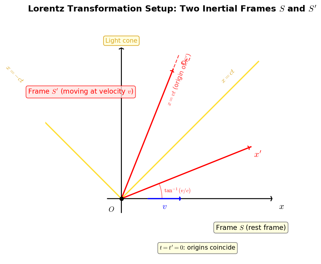
Fig. 5.2: Spacetime diagram of the Lorentz transformation. The coordinate axes of inertial frame \(S\) (black) and those of \(S'\) moving at velocity \(v\) (blue). The time and space axes of \(S'\) tilt symmetrically, while the worldline of light \(x = ct\) maintains 45° in both frames.
For \(v \ll c\), \(\gamma \approx 1\), recovering the Galilean transformation. As \(v \to c\), \(\gamma\) diverges — looking at Fig. 5.3 "Velocity dependence of the Lorentz factor γ", you can see it's nearly 1 at everyday speeds but shoots up dramatically near the speed of light. Geometrically, using the rapidity \(\varphi\) (\(\tanh\varphi = v/c\)), it can be written as a hyperbolic rotation in the \(t\)-\(x\) plane (see General Relativity Ch. 3 for details).
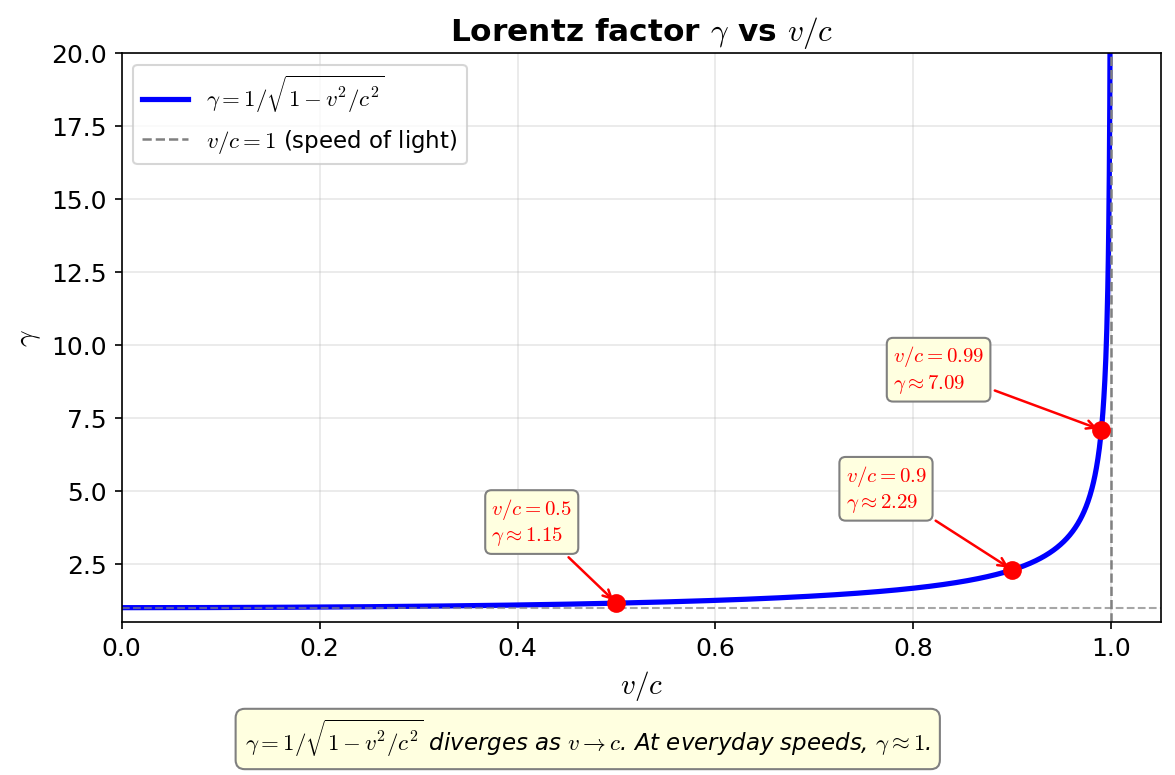
Fig. 5.3: Velocity dependence of the Lorentz factor γ. \(\gamma = 1/\sqrt{1-v^2/c^2}\) diverges as \(v \to c\). At everyday speeds, \(\gamma \approx 1\).
Physical Consequences (General Relativity Ch. 3)
Table 5.1: Main physical consequences of the Lorentz transformation
| Phenomenon | Formula | Meaning |
|---|---|---|
| Relativity of simultaneity | \(\Delta t' = -\gamma(v/c^2)\Delta x\) (when \(\Delta t = 0\)) | Two events simultaneous and separated in \(S\) are not simultaneous in \(S'\) |
| Time dilation | \(\Delta t = \gamma\,\Delta t'\) | A moving clock runs slower |
| Length contraction | \(L = L_0/\gamma\) | A moving rod appears shorter in the direction of motion |
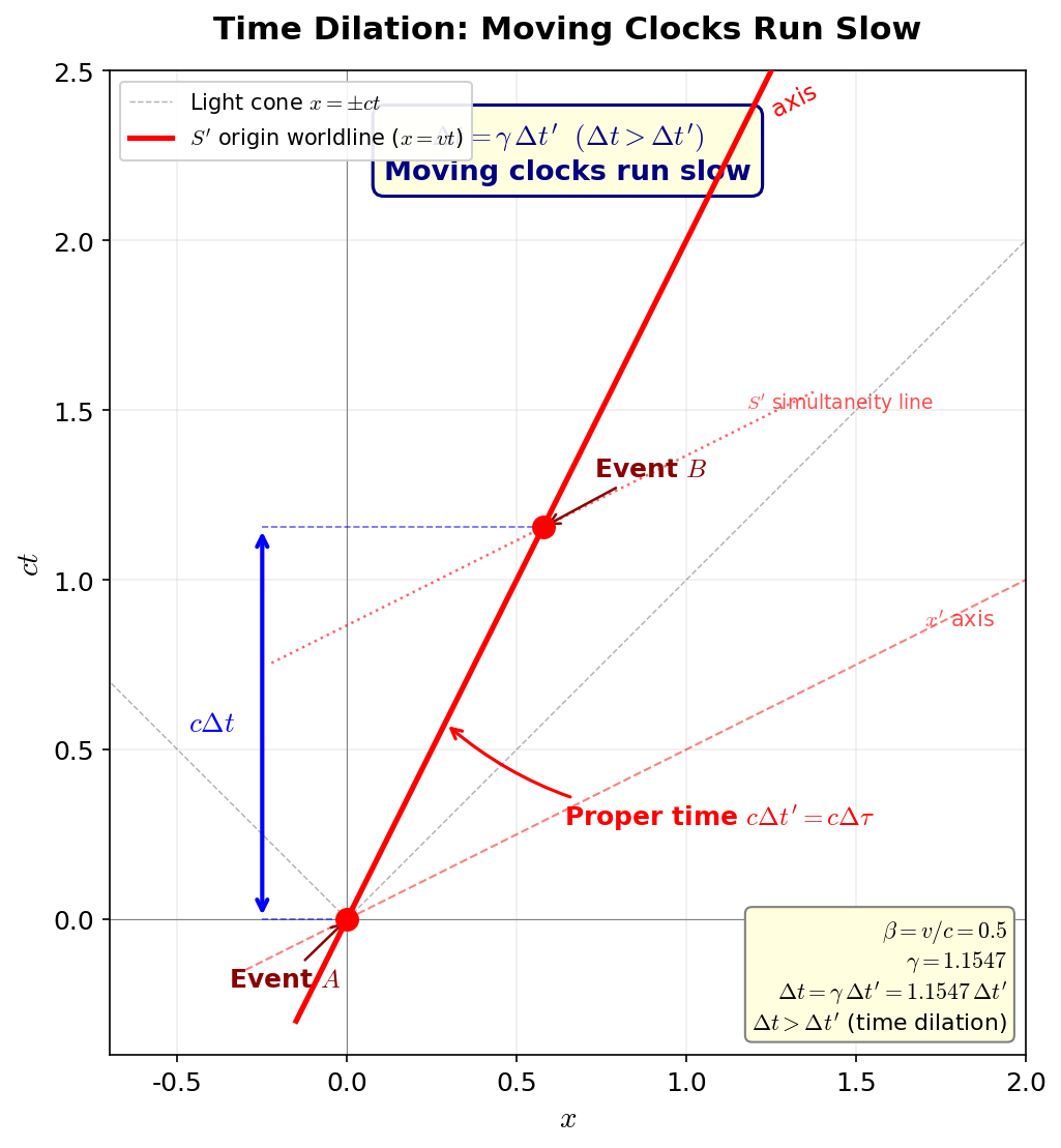
Fig. 5.4: Time dilation. The proper time \(\Delta t'\) ticked by a clock in the moving frame \(S'\) is stretched to \(\Delta t = \gamma\,\Delta t' > \Delta t'\) as observed in the rest frame \(S\). The closer the speed is to the speed of light, the more pronounced the dilation.
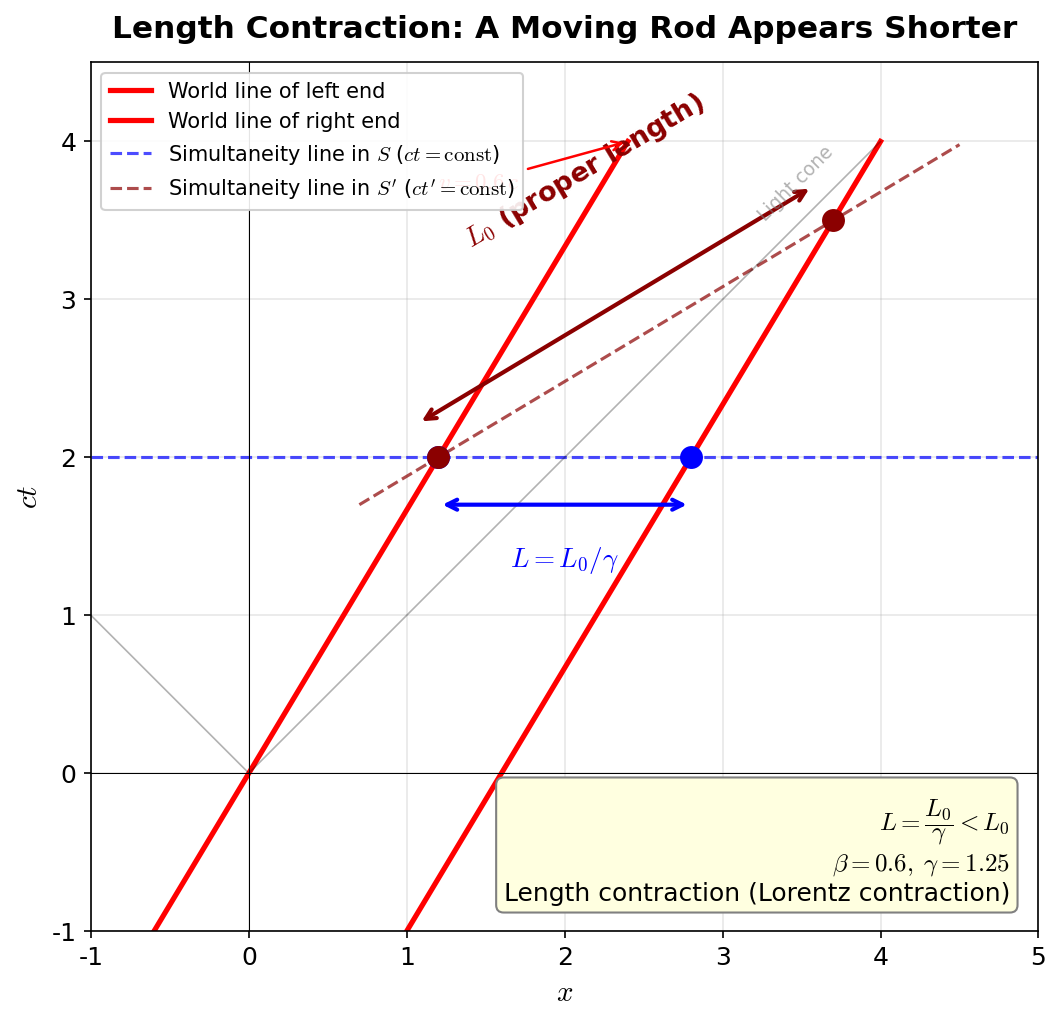
Fig. 5.5: Length contraction. A rod of rest length \(L_0\) is observed to be contracted to \(L = L_0/\gamma < L_0\) when moving at velocity \(v\). The contraction occurs only in the direction of motion.
🔵 Kai: "If \(S\) sees \(S'\)'s clock running slow, then \(S'\) should also see \(S\)'s clock running slow" — that's the twin paradox, right? If they both say "the other one is running slow," who ends up younger?
🟡 Lina: The one who rode the rocket ends up younger — that settles it. The one who experiences acceleration switches inertial frames, which breaks the symmetry between the two. See the Dive Deep section in General Relativity Ch. 3 for details. Muon lifetimes and GPS time corrections are also covered there.
🔵 Kai: The symmetry breaks the moment one accelerates... So does the age difference depend on "how much acceleration" and "how long the acceleration lasts"?
🟡 Lina: Exactly. The difference in proper time is determined by integrating over the entire path. Even with the same departure and arrival points, the age difference changes between a route with violent acceleration and a gentle route. The quantitative calculation is in the Dive Deep section of General Relativity Ch. 3.
🔵 Kai: "Integrating over the entire path" — so basically you add up all the acceleration along the way and compare?
⚪ Mei: So "both being equivalent" only holds while both are in inertial frames. The moment one accelerates, the situation becomes asymmetric.
✅ Comprehension Check: Why does the twin paradox resolve with "the one who rode the rocket is younger"?
Answer
The one who rode the rocket experiences acceleration (deceleration, turnaround), switching between inertial frames. This breaks the symmetry of the two situations, so the elapsed time for the one who experienced acceleration is shorter, and they remain younger.
5.3 Tools of Minkowski Spacetime (What We Use in String Theory)
🟡 Lina: In string theory, we'll work with spacetimes that have more than just 4 dimensions (why the number of dimensions increases will become clear from Ch. 14 onward). As the simplest case first, we take the background spacetime in which strings move to be \(D\)-dimensional flat Minkowski spacetime. Since even in curved spacetime the neighborhood of each point can be approximated by Minkowski spacetime (the local flatness theorem, see General Relativity Ch. 7), the tools we develop here will be used all the way to the end. In this section, I'll write specific formulas in 4 dimensions (\(D = 4\)), but generalization to \(D\) dimensions is straightforward — the coordinates simply increase to \(x^0, x^1, \ldots, x^{D-1}\), and in light-cone coordinates the transverse components become the \(D - 2\) components \(x^2, x^3, \ldots, x^{D-1}\). Let me list the key points.
Unit System and Sign Convention
From this section onward, we use natural units with \(c = 1\) as our default (see General Relativity Ch. 4). Time and space are measured in the same units, and \(c\) is not written explicitly in formulas. In string theory, we often additionally set \(\hbar = \alpha' = 1\), but we'll introduce that when needed. When SI numerical values are needed, we restore \(c\) through dimensional analysis.
Sign convention: We adopt the same convention as General Relativity, \(\eta_{\mu\nu} = \mathrm{diag}(-1, +1, +1, +1)\) (mostly plus). In Quantum Field Theory we used \((+,-,-,-)\) (mostly minus), but since standard string theory textbooks (Zwiebach, Polchinski, etc.) adopt mostly plus, we unify with that convention here.
Coordinates and Indices (General Relativity Ch. 4)
Einstein summation convention: When the same index appears both up and down, sum over it. \(A^\mu B_\mu \equiv \sum_\mu A^\mu B_\mu\).
Minkowski Metric (General Relativity Ch. 4)
An invariant quantity that takes the same components in all inertial frames. Restoring \(c\): \(ds^2 = -c^2 dt^2 + dx^2 + dy^2 + dz^2\).
4-Momentum and the Energy-Momentum Relation (General Relativity Ch. 4)
The 4-momentum of a particle (\(U^\mu\) is the 4-velocity, see General Relativity Ch. 4):
From the invariant norm \(p^\mu p_\mu = -m^2\), the energy-momentum relation is
(Why the minus sign in \(-m^2\): \(p^\mu p_\mu = \eta_{\mu\nu}p^\mu p^\nu = -E^2 + |\vec{p}|^2\), where the minus on the energy term comes from \(\eta_{00} = -1\). For a particle at rest with \(\vec{p} = 0\), \(p^\mu p_\mu = -E^2 = -m^2\), which is consistent.)
- At rest: \(E = m\) (restoring SI units: \(E = mc^2\))
- Low-speed limit: \(E \approx m + \frac{1}{2}m v^2\) (in SI: \(E \approx mc^2 + \frac{1}{2}mv^2\); see General Relativity Ch. 4 for the expansion)
- Zero mass: \(E = |\vec{p}|\), always travels at the speed of light
🔵 Kai: It's still amazing that something has energy \(m\) just by sitting still.
🟡 Lina: If we graph this relation, it forms a hyperbola (Fig. 5.6 "Geometric representation of the energy-momentum relation \(E^2 = p^2 + m^2\)"). The set of points satisfying \(E^2 - |\vec{p}|^2 = m^2\) traces out a hyperbola. Since a particle must always lie on this curve, it's called the mass shell — meaning "the shell on which the particle sits." Massless light lies on the straight line \(E = |p|\), while massive particles lie on the hyperbola.
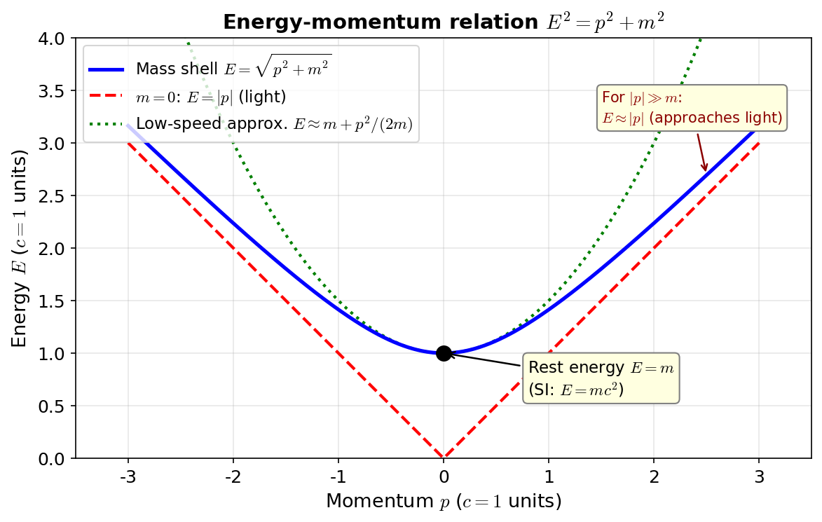
Fig. 5.6: Geometric representation of the energy-momentum relation \(E^2 = p^2 + m^2\). Particles sit on the mass shell (hyperbola), and for \(m = 0\), light coincides with the line \(E = |p|\). At low speeds, it reduces to the parabolic approximation (kinetic energy in Newtonian mechanics).
✅ Comprehension Check: In \(E^2 = |\vec{p}|^2 + m^2\) (with \(c=1\)), what is the energy when a particle is at rest (\(\vec{p}=0\))?
Answer
\(E = m\) (in natural units with \(c=1\)). Restoring SI units gives \(E = mc^2\). This is the famous mass-energy equivalence relation.
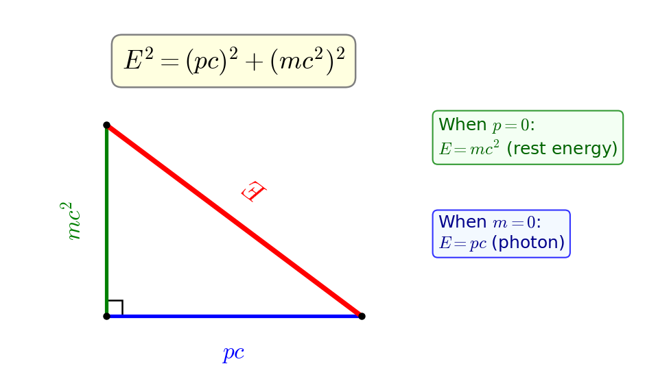
Fig. 5.7: Energy-momentum triangle relation. \(E^2 = |\vec{p}|^2 + m^2\) (with \(c = 1\)) can be visualized as the Pythagorean theorem of a right triangle. Taking the rest energy \(m\) as the base and the momentum \(|\vec{p}|\) as the height, the hypotenuse corresponds to the total energy \(E\).
🔵 Kai: The property of being massless and traveling at the speed of light — that's the one we'll use again when gravitons appear in string theory (Ch. 15), right? But \(E = \sqrt{|\vec{p}|^2 + m^2}\) has a square root, so it seems hard to handle when quantizing, doesn't it?
🟡 Lina: That's precisely the problem. In the next section, we'll introduce coordinates — light-cone coordinates — where this energy-momentum relation can be solved as a linear equation. Thanks to that, \(p^-\) is uniquely determined from the other components, making quantization of the string dramatically easier.
🔵 Kai: A square root means there's also a negative solution \(E = \pm\sqrt{|\vec{p}|^2 + m^2}\), right? What does negative energy mean?
🟡 Lina: Good question. Mathematically, the solution \(p^0 = -\sqrt{|\vec{p}|^2 + m^2}\) exists. The physical interpretation is understood as antiparticles in quantum field theory (Quantum Field Theory), but for now just remember the mathematical inconvenience that "taking the square root gives two solutions \(\pm\)." The key point of light-cone coordinates is that this \(\pm\) disappears.
📖 Returning to previously learned material: For the distinction between contravariant and covariant vectors, raising and lowering indices \(A_\mu = \eta_{\mu\nu}A^\nu\), and tensor contraction and rank, see General Relativity Ch. 4. When we handle tensors on the string worldsheet from Chapter 13 onward, we'll naturally carry over the notation from there.
5.4 Light-Cone Structure and Light-Cone Coordinates — The Star of String Theory
🟡 Lina: Here begins the original content of this chapter. Light-cone coordinates are the key tool for most quickly identifying "which degrees of freedom are physical" in string quantization (Ch. 14). Let's first briefly review the light-cone structure (causality) as preparation, then define the light-cone coordinates.
Review of Light-Cone Structure (Causality)
🟡 Lina: The sign of \(ds^2\) between two events classifies their causal relationship into three types.
Table 5.2: Causal classification by the sign of the spacetime interval
| Sign of \(ds^2\) | Name | Physical Meaning |
|---|---|---|
| \(ds^2 < 0\) | Timelike | Can be connected by a subluminal signal. Causally related |
| \(ds^2 = 0\) | Null / Lightlike | Can be connected by light. On the light cone |
| \(ds^2 > 0\) | Spacelike | Cannot be connected even by light. No causal relation |
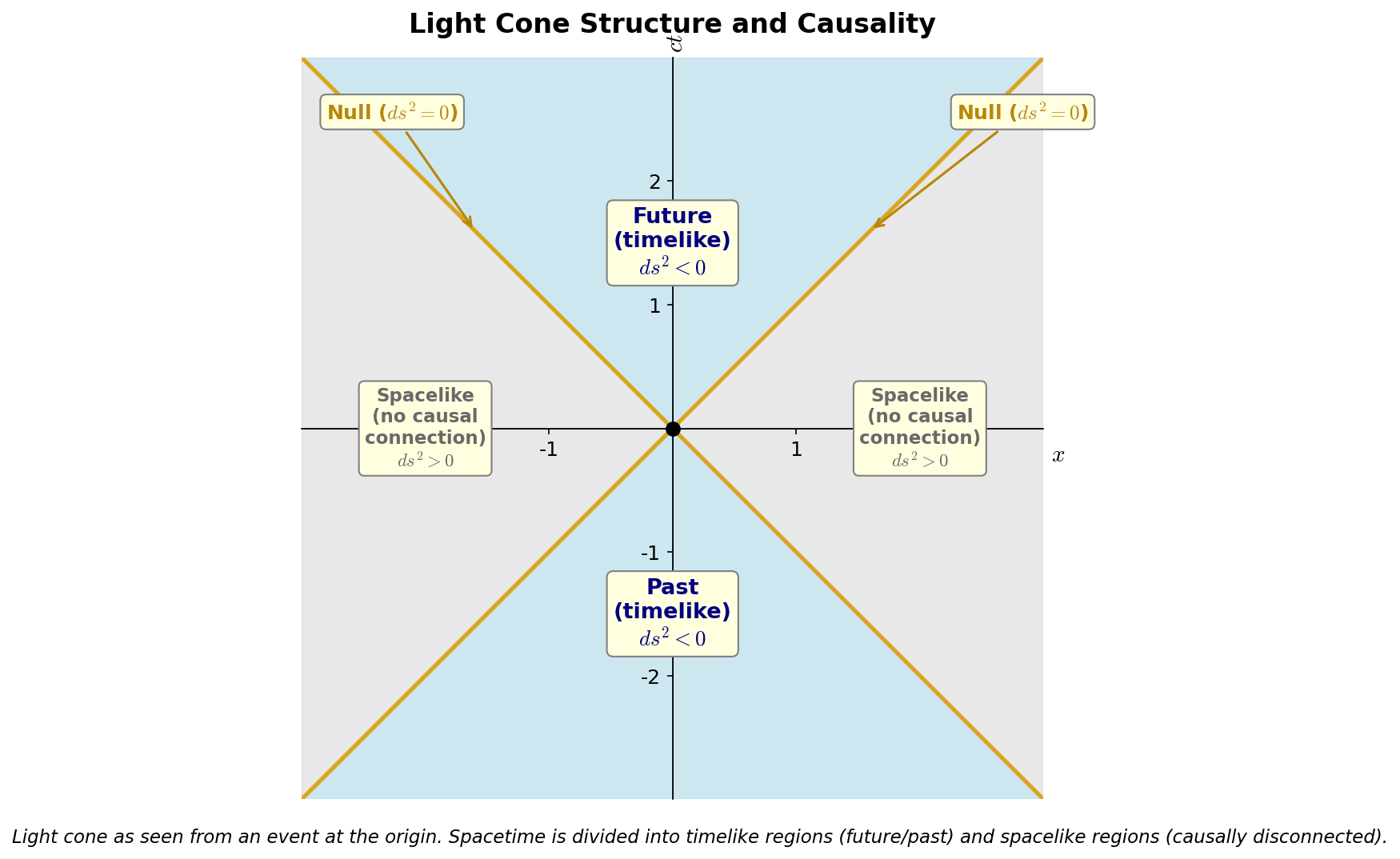
Fig. 5.8: Light-cone structure and causality. The light cone as seen from the event at the origin. Spacetime is divided into timelike regions (future and past) and spacelike regions (causally unrelated).
The surface \(ds^2 = 0\) forms the light cone, dividing spacetime into past, future, and causally unrelated regions (Fig. 5.8 "Light-cone structure and causality"). See "Three classifications of spacetime intervals" in General Relativity Ch. 3 for details.
Definition of Light-Cone Coordinates
🟡 Lina: We define new coordinates by combining the time coordinate \(x^0\) with one of the spatial coordinates \(x^1\):
The remaining coordinates \(x^2, x^3\) stay as they are.
🔵 Kai: Why is it called "light-cone" coordinates?
🟡 Lina: Consider light departing from the origin and traveling only in the \(x^1\) direction: \(dx^2 = dx^3 = 0\), and from \(ds^2 = 0\) we get \(-(dx^0)^2 + (dx^1)^2 = 0\), meaning \(dx^0 = \pm dx^1\). Light traveling in the positive direction satisfies \(dx^0 = dx^1\), so integrating gives \(x^0 = x^1 + C\) (\(C\) is a constant). Starting from the origin means \(C = 0\), so \(x^1 = x^0\) (in natural units with \(c = 1\)). Then
Light in the opposite direction has \(x^1 = -x^0\), giving \(x^+ = \frac{1}{\sqrt{2}}(x^0 + x^1) = 0\). In other words, along the worldline of light emitted from the origin, either \(x^+\) or \(x^-\) takes a constant value (0).
⚪ Mei: It's zero for light starting from the origin, but does the same thing hold for light starting from other points?
🟡 Lina: Good check. Light traveling in the \(x^1\) direction always satisfies \(dx^0 = \pm dx^1\), so \(dx^- = \frac{1}{\sqrt{2}}(dx^0 - dx^1) = 0\) (positive direction) or \(dx^+ = 0\) (negative direction). That is, along a light worldline, either \(x^+\) or \(x^-\) is constant (the constant value isn't necessarily 0, but it doesn't change). By the way, as we saw in Fig. 5.8 "Light-cone structure and causality", the light cone literally has the shape of a "cone" — if you draw the spacetime diagram of light spreading in all directions from the origin, it forms the surface of a cone. The straight lines you can draw from the apex of the cone along its surface are called generators (generatrices).
🔵 Kai: Generators? I think I've heard that before... are those the straight lines that make up the surface of a cone?
🟡 Lina: Yes. A generator is a straight line that constitutes the surface of a cone — a line you can draw straight from the apex along the surface. Imagine placing a ruler from the pointed tip of an ice cream cone toward the rim — that's a generator. Since a light cone is a type of cone, the straight lines drawn from the apex (the event at the origin) in the direction light travels are the generators of the light cone. It's called "light-cone coordinates" because they are coordinates along the generators of the light cone. It's easier to see in a figure (Fig. 5.9 "Geometric meaning of light-cone coordinates") — you can see that it's the usual \((x^0, x^1)\) coordinates rotated by 45 degrees, and the worldlines of light coincide exactly with the new coordinate axes.
🔵 Kai: A straight line from placing a ruler on the cone's surface... I see, it's like the "skeleton" of the cone. And the trajectory of light corresponds to each of those skeletal lines. So the \(x^+\) axis and \(x^-\) axis are choosing two of those skeletal lines — specifically the ones for light going in the positive and negative \(x^1\) directions?
🟡 Lina: Exactly. The light cone has generators in all directions, but we focus on the \(x^1\) direction, choose two lines, and make them the new coordinate axes — that's light-cone coordinates.
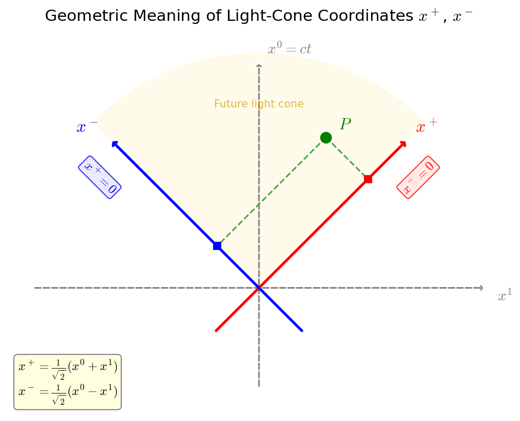
Fig. 5.9: Geometric meaning of light-cone coordinates. A coordinate system obtained by rotating the usual \((x^0, x^1)\) coordinates by 45 degrees. The worldlines of light coincide with the coordinate axes.
🔵 Kai: Ah, looking at Fig. 5.9 "Geometric meaning of light-cone coordinates", the \(x^+\) and \(x^-\) axes are indeed along the light directions.
🔵 Kai: Why is there a factor of \(1/\sqrt{2}\)? Wouldn't \(x^+ = x^0 + x^1\) work?
🟡 Lina: Good question. If we define \(\tilde{x}^+ = x^0 + x^1\) and \(\tilde{x}^- = x^0 - x^1\) without the \(1/\sqrt{2}\), then \(d\tilde{x}^+ d\tilde{x}^- = (dx^0)^2 - (dx^1)^2\), so \(ds^2 = -d\tilde{x}^+ d\tilde{x}^- + (dx^2)^2 + (dx^3)^2\). When we write \(ds^2 = \tilde{\eta}_{\mu\nu}\,d\tilde{x}^\mu d\tilde{x}^\nu\), Einstein's summation convention sums over all combinations of \(\mu\) and \(\nu\).
🔵 Kai: "All combinations" — how does that expand out concretely?
🟡 Lina: For example, with coordinates \((\tilde{x}^+, \tilde{x}^-, \tilde{x}^2, \tilde{x}^3)\) — four coordinates — \(\mu\) takes values \(+, -, 2, 3\) and \(\nu\) also takes \(+, -, 2, 3\), giving \(4 \times 4 = 16\) terms to sum. Among those, picking out the terms involving both \(+\) and \(-\), we get two: the term with \(\mu = +, \nu = -\) and the term with \(\mu = -, \nu = +\).
🔵 Kai: Two terms appear because \(\mu\) and \(\nu\) run independently.
🟡 Lina: Right. So we get two terms: \(\tilde{\eta}_{+-}d\tilde{x}^+ d\tilde{x}^- + \tilde{\eta}_{-+}d\tilde{x}^- d\tilde{x}^+\). The metric tensor is symmetric (\(\tilde{\eta}_{+-} = \tilde{\eta}_{-+}\)), and \(d\tilde{x}^+ d\tilde{x}^-\) equals \(d\tilde{x}^- d\tilde{x}^+\) (they're just products of numbers, so order doesn't matter), giving a combined \(2\tilde{\eta}_{+-}\,d\tilde{x}^+ d\tilde{x}^-\). This must equal \(-d\tilde{x}^+ d\tilde{x}^-\), so \(2\tilde{\eta}_{+-} = -1\), meaning \(\tilde{\eta}_{+-} = -1/2\).
🔵 Kai: \(-1/2\) is indeed an awkward number. What happens with the \(1/\sqrt{2}\)?
🟡 Lina: With the \(1/\sqrt{2}\) definition — as I'll derive shortly — we get \(ds^2 = -2\,dx^+ dx^- + \cdots\). Let's write the metric components in light-cone coordinates as \(\hat{\eta}_{\mu\nu}\). Even though it's the same Minkowski metric, the numerical values of the components change when coordinates change (just as changing how you draw a map changes the spacing of latitude and longitude lines). We put the hat (\(\hat{}\)) to distinguish from the standard-coordinate \(\eta_{\mu\nu} = \mathrm{diag}(-1,+1,+1,+1)\). Doing the same expansion as before, in \(\hat{\eta}_{\mu\nu}\,dx^\mu dx^\nu\) the terms involving \(+\) and \(-\) give \(2\hat{\eta}_{+-}\,dx^+dx^-\). Setting this equal to \(-2\,dx^+dx^-\) gives \(2\hat{\eta}_{+-} = -2\), meaning \(\hat{\eta}_{+-} = -1\) exactly.
⚪ Mei: To summarize: without \(1/\sqrt{2}\) we get the awkward \(\tilde{\eta}_{+-} = -1/2\), but with \(1/\sqrt{2}\) we get the clean \(\hat{\eta}_{+-} = -1\).
🟡 Lina: That's right. Since the metric components become only \(\pm 1\) or \(0\), raising and lowering indices becomes easy. I'll write out the full matrix shortly. Now let's actually derive \(ds^2 = -2\,dx^+dx^-\).
Spacetime Interval in Light-Cone Coordinates
🟡 Lina: Let's rewrite \(ds^2\) in light-cone coordinates. The starting point is the Minkowski metric in standard coordinates:
We want to replace the \(-(dx^0)^2 + (dx^1)^2\) part with light-cone coordinates. From the definitions:
Computing the product:
So \((dx^0)^2 - (dx^1)^2 = 2\,dx^+ dx^-\). What appears in \(ds^2\) is \(-(dx^0)^2 + (dx^1)^2\) with the opposite sign, so multiplying both sides by \(-1\):
Substituting into \(ds^2\):
(Here \((dx^2)^2\) means "the square of the infinitesimal change \(dx^2\) of coordinate \(x^2\)." The superscript 2 is the coordinate label, not an exponent, so although it's confusing, read \((dx^2)^2 = (dx^2) \times (dx^2)\). Same for \((dx^3)^2\).)
🔵 Kai: Wait, in the original formula \((dx^0)^2\) and \((dx^1)^2\) appeared separately, but in light-cone coordinates \(dx^+\) and \(dx^-\) appear as a product. How is a product intuitively different from a sum of squares?
🟡 Lina: Good question. With a sum of squares, each direction contributes independently, but with a product, if one factor is zero the whole thing vanishes. In other words, if one coordinate doesn't change, that term disappears entirely. For example, moving only in the \(x^+\) direction (\(dx^- = 0\), \(dx^2 = dx^3 = 0\)) gives \(ds^2 = -2\,dx^+\cdot 0 + 0 + 0 = 0\). Since \(ds^2 = 0\) is the condition for light, this is consistent with what we said about light's worldline lying along the \(x^+\) axis.
🔵 Kai: Ah, I see. In standard coordinates, finding the condition \(ds^2 = 0\) requires the calculation "\(-(dx^0)^2 + (dx^1)^2 = 0\) so \(dx^0 = \pm dx^1\)," but in light-cone coordinates you can just say "\(dx^-\) is zero" in one shot.
⚪ Mei: Right — it's precisely because of the product structure that the correspondence "one coordinate being constant = light" is directly visible.
🟡 Lina: I already used this in the \(1/\sqrt{2}\) discussion earlier, but let me organize it again. Let me say the important thing first: the physical spacetime is the same Minkowski spacetime — all that changed is how we chose coordinates. But when coordinates change, the "numerical values of the components" of the metric tensor change (just as changing the map projection changes the spacing of grid lines). To avoid confusion, I'll write the components expressed in light-cone coordinates as \(\hat{\eta}_{\mu\nu}\) (the hat is just a marker meaning "expressed in light-cone coordinates," not a different metric). We're just distinguishing it from the numerical values \(\eta_{\mu\nu} = \mathrm{diag}(-1,+1,+1,+1)\) in standard coordinates. One note here — in light-cone coordinates, the coordinates are \((x^+, x^-, x^2, x^3)\), so the index \(\mu\) takes the four values \(+, -, 2, 3\) rather than \(0, 1, 2, 3\). We've been using this implicitly since defining \(x^+, x^-\), but let me make it explicit here. Only the labels change; the role of "labels distinguishing four directions" remains the same.
🔵 Kai: I see — the index labels just change from numbers to \(+, -\), but the essence of having four directions is the same.
🟡 Lina: Right. Taking the row and column order as \(+, -, 2, 3\):
Check the position of each component in the left matrix. For example, row 1, column 2 is \(\hat{\eta}_{+-}\), and looking at the right matrix its value is \(-1\). The diagonal components \(\hat{\eta}_{++}\) and \(\hat{\eta}_{--}\) are zero, and the off-diagonal components \(\hat{\eta}_{+-} = \hat{\eta}_{-+} = -1\) remain. In the Minkowski metric where "time is minus, space is plus," here everything is consolidated into the \(+\) and \(-\) combination.
⚪ Mei: The \(-1\) that was on the diagonal has moved off-diagonal. It's an unfamiliar form, but the components being only \(0, \pm 1\) is certainly clean.
🟡 Lina: The inverse metric (the matrix used to raise indices) \(\hat{\eta}^{\mu\nu}\) is determined by \(\hat{\eta}^{\mu\alpha}\hat{\eta}_{\alpha\nu} = \delta^\mu_\nu\). In this case, the numerical values happen to be the same as \(\hat{\eta}_{\mu\nu}\): \(\hat{\eta}^{+-} = \hat{\eta}^{-+} = -1\), \(\hat{\eta}^{22} = \hat{\eta}^{33} = +1\), all others 0. The reason they're the same is that multiplying the above matrix by itself gives the identity matrix (it's its own inverse). I'll leave the verification as a practice problem.
4-Momentum in Light-Cone Coordinates
🟡 Lina: In light-cone coordinates, the components of 4-momentum also become
(Fig. 5.10 "Decomposition of momentum in light-cone coordinates"). In the usual \((p^0, p^1)\) plane, the \(p^+\) and \(p^-\) axes correspond to the generator directions of the light cone — that is, directions tilted at 45 degrees. The hyperbola in the figure is the mass shell, and particles always lie on it. In light-cone coordinates, once you fix the value of \(p^+\), the point on the hyperbola is uniquely determined — meaning \(p^-\) is determined as a dependent variable.
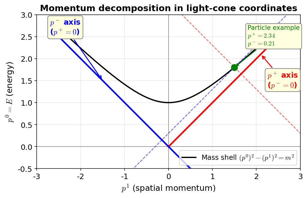
Fig. 5.10: Decomposition of momentum in light-cone coordinates. The \(p^+\) and \(p^-\) axes are overlaid on the usual \((p^0, p^1)\) plane. For a particle on the mass shell (hyperbola), \(p^-\) is uniquely determined by \(p^+\) and the transverse momenta.
🟡 Lina: Now let's write \(p^\mu p_\mu = -m^2\) in light-cone coordinates. The algebra is exactly the same as when we showed \((dx^0)^2 - (dx^1)^2 = 2\,dx^+dx^-\) for \(ds^2\). In standard coordinates, we lower indices with \(p_\mu = \eta_{\mu\nu}p^\nu\) (see General Relativity Ch. 4), so \(p^\mu p_\mu = \eta_{\mu\nu}p^\mu p^\nu = -(p^0)^2 + (p^1)^2 + (p^2)^2 + (p^3)^2\). In light-cone coordinates the same mechanism applies: we compute \(p^\mu p_\mu = \hat{\eta}_{\mu\nu}\,p^\mu p^\nu\) using the metric tensor components (for instance, \(p_+ = \hat{\eta}_{+-}p^- + \hat{\eta}_{++}p^+ = -p^-\) shows how indices are lowered, but for now it's faster to directly substitute the components of \(\hat{\eta}_{\mu\nu}\)). From the definitions of \(p^+\) and \(p^-\):
so \((p^0)^2 - (p^1)^2 = 2\,p^+ p^-\). Substituting: \(-(p^0)^2 + (p^1)^2 = -2\,p^+ p^-\), so
🔵 Kai: It's exactly the same structure as the \(ds^2\) case. You just replaced the infinitesimal coordinate changes \(dx^\mu\) with momenta \(p^\mu\).
🟡 Lina: Exactly. (Expanding the double sum, the only nonzero components of \(\hat{\eta}_{\mu\nu}\) are \(\hat{\eta}_{+-} = \hat{\eta}_{-+} = -1\) and \(\hat{\eta}_{22} = \hat{\eta}_{33} = +1\), so the surviving terms are four: \(\hat{\eta}_{+-}p^+p^- + \hat{\eta}_{-+}p^-p^+ + \hat{\eta}_{22}p^2 p^2 + \hat{\eta}_{33}p^3 p^3\). Since \(p^+, p^-, p^2, p^3\) are just numbers (not operators), we can swap the order of products: \(p^-p^+ = p^+p^-\). So \(= (-1)p^+p^- + (-1)p^+p^- + (p^2)^2 + (p^3)^2 = -2p^+p^- + (p^2)^2 + (p^3)^2\). The diagonal components \(\hat{\eta}_{++} = \hat{\eta}_{--} = 0\), so all other terms vanish.)
Here \((p^2)^2\) means "the square of \(p^2\) (the second component of momentum)." Since the index 2 and the exponent 2 are confusing, we sometimes use uppercase Latin indices like \((p^I)^2\) (\(I = 2, 3\)) when needed. \(p^2\) and \(p^3\) are the components in the directions we didn't touch when defining light-cone coordinates — they're transverse (perpendicular) to the \(x^+, x^-\) axes — so we collectively write them as the transverse momentum \(\vec{p}_\perp = (p^2, p^3)\). \((p^2)^2 + (p^3)^2 = |\vec{p}_\perp|^2\). We'll use this notation in later chapters too.
🔵 Kai: It's definitely confusing... whether \(p^2\) means "\(p\) squared" or "the second component." The \(\vec{p}_\perp\) notation is more reassuring.
🟡 Lina: Right. I'll use \(\vec{p}_\perp\) when there's ambiguity, so don't worry. Now let's solve for \(p^-\). Rearranging \(-2p^+p^- + |\vec{p}_\perp|^2 = -m^2\) gives \(2p^+p^- = |\vec{p}_\perp|^2 + m^2\), and dividing both sides by \(2p^+\):
(where \(|\vec{p}_\perp|^2 = (p^2)^2 + (p^3)^2\).)
🔵 Kai: It's solvable! \(p^-\) is determined by the other components (\(p^+, p^2, p^3\) and the mass). So one independent variable is reduced — in standard coordinates you needed a square root to find \(E\), but here it's just a single division. But wait — if \(p^+\) is zero, the denominator is zero and it diverges, right? What does that mean?
🟡 Lina: Good eye. Since \(p^+ = \frac{1}{\sqrt{2}}(E + p^1)\), for a massive particle choosing the positive-energy solution (\(E > 0\)), we have \(E > |p^1|\). Tracing through carefully: \(|\vec{p}|^2 = (p^1)^2 + (p^2)^2 + (p^3)^2\), and since \((p^2)^2\) and \((p^3)^2\) are non-negative, \(|\vec{p}|^2 \geq (p^1)^2\). Therefore \(E^2 = |\vec{p}|^2 + m^2 \geq (p^1)^2 + m^2 > (p^1)^2\). Since we chose the positive-energy solution \(E > 0\), taking positive square roots of both sides: \(E = \sqrt{E^2} > \sqrt{(p^1)^2} = |p^1|\) (for positive numbers \(a, b\), if \(a^2 > b^2\) then \(a > b\); apply with \(a = E > 0\) and \(b = |p^1| \geq 0\)). Since \(E > |p^1|\) means \(E > -p^1\) (even if \(p^1\) is negative), we get \(E + p^1 > 0\), so \(p^+ > 0\) always.
⚪ Mei: As long as there's mass, positive energy guarantees \(p^+\) is positive — no worry about the denominator being zero.
🟡 Lina: Right. \(p^+ = 0\) corresponds to a massless particle traveling at exactly the speed of light in the negative \(x^1\) direction (\(E = |p^1|\) with \(p^1 < 0\) giving \(E + p^1 = 0\)). In light-cone quantization, we adopt the convention of only considering particles with \(p^+ > 0\), avoiding this issue. In standard coordinates, \(p^\mu p_\mu = -(p^0)^2 + |\vec{p}|^2 = -m^2\) gives \(p^0 = \pm\sqrt{|\vec{p}|^2 + m^2}\) with a \(\pm\) sign ambiguity (\(p^0 > 0\) is the positive-energy solution = normal particle, \(p^0 < 0\) is the negative-energy solution). But in light-cone coordinates, \(p^-\) is uniquely determined by a linear equation.
⚪ Mei: The sign ambiguity disappears.
🟡 Lina: That's right. This is the reason why light-cone quantization in Ch. 14 can pick out only the physical states from the start.
🟡 Lina: Let me put the comparison between standard and light-cone coordinates in a table.
Table 5.3: Comparison of standard and light-cone coordinates
| Item | Standard coordinates \((x^0, x^1, x^2, x^3)\) | Light-cone coordinates \((x^+, x^-, x^2, x^3)\) |
|---|---|---|
| Definition | \(x^0 = t\), \(x^1 = x\) | \(x^\pm = (x^0 \pm x^1)/\sqrt{2}\) |
| Metric \(ds^2\) | \(-(dx^0)^2 + (dx^1)^2 + (dx^2)^2 + (dx^3)^2\) | \(-2\,dx^+dx^- + (dx^2)^2 + (dx^3)^2\) |
| Metric tensor | \(\eta_{\mu\nu} = \mathrm{diag}(-1,+1,+1,+1)\) | \(\hat{\eta}_{+-} = -1\), \(\hat{\eta}_{22} = \hat{\eta}_{33} = +1\), others 0 |
| Energy-momentum | $E = \pm\sqrt{ | \vec{p} |
| Sign ambiguity | \(\pm\) present (positive/negative energy solutions) | None (unique once \(p^+\) is fixed positive) |
| Light worldline | \(x^1 = \pm x^0\) (slope \(\pm 1\)) | \(x^+ = \text{const}\) or \(x^- = \text{const}\) |
Preview of the Benefits for String Theory
🔵 Kai: In the end, what's the benefit of using light-cone coordinates? There must be enough payoff to justify the trouble of changing coordinates, right?
🟡 Lina: We'll use them fully in Ch. 14 (string quantization), but as a preview, here are three points. For now, just getting the general feel is enough.
- \(p^-\) becomes a dependent variable: As we saw above. The number of degrees of freedom is reduced.
- Removing extra degrees of freedom becomes easy: When a point particle moves through spacetime, it traces a 1-dimensional trajectory = worldline. Similarly, when a 1-dimensional string moves, it traces a 2-dimensional surface — called the worldsheet. This worldsheet has "freedom in how you choose coordinates" that doesn't affect the physics — just as changing how you draw a map doesn't change the terrain, the physics doesn't change regardless of how you parametrize the worldsheet. But when doing calculations, you have to choose some specific coordinates, so information about "which coordinates you chose" — which is irrelevant to physics — creeps into the equations. Then among the solutions of the equations, a huge number of "states that are physically identical, just with a different choice of coordinates" get mixed in, making it impossible to tell which are the genuine physical degrees of freedom. Using light-cone coordinates, you can make a natural choice (light-cone gauge) that aligns the worldsheet "time direction" parameter \(\tau\) with \(x^+\), fixing that redundancy all at once. As a result, only the transverse oscillations \(x^2, x^3, \ldots\) remain as physical degrees of freedom.
🔵 Kai: The worldsheet is the "surface traced by the string's motion," right? Just as a moving point becomes a line, a moving line becomes a surface. The map analogy makes sense, but can I wait until Ch. 14 for the concrete meaning of "light-cone gauge"?
🟡 Lina: Yes, for now just remember the conclusion that "light-cone coordinates let you eliminate extra degrees of freedom." We'll go through the concrete steps in Ch. 14.
- The physical spectrum is obtained directly: In the standard method, non-physical states where "probability becomes negative" appear midway through the calculation, and must be removed afterward. Light-cone coordinates exclude such states from the start.
⚪ Mei: Reducing degrees of freedom and excluding non-physical states — that's quite powerful.
🟡 Lina: However, there is a trade-off. Lorentz covariance is explicitly lost (because we're treating \(x^+\) specially). But since physical results are independent of coordinate system, it's not a problem — this is the basic property of relativity that "computing in a specific coordinate system still yields general results."
🔵 Kai: But Lorentz covariance means "the laws of physics have the same form in every inertial frame," right? Is explicitly losing that really okay? Isn't there a danger of overlooking something along the way?
🟡 Lina: That's a sharp concern. In practice, light-cone quantization requires a final check that "Lorentz symmetry is truly preserved." The condition for that check to succeed determines the spacetime dimension to be \(D = 26\) (bosonic string) or \(D = 10\) (superstring) — a major result we'll see in Ch. 14. So "confirming the hidden covariance at the end" is a step that comes as part of the package.
⚪ Mei: Making covariance invisible to simplify the calculation, then checking covariance at the end — and from that the spacetime dimension is determined.
🔵 Kai: So it's like "paying the debt for taking the easy route at the end," and from paying that debt the dimension is determined... But conversely, if the dimension weren't 26 or 10, Lorentz symmetry would be broken, right? Can that be tested experimentally?
🟡 Lina: Good question. How extra dimensions might be experimentally observable is covered in Ch. 16. At this stage, just remember that "light-cone coordinates are the first step in trading covariance for calculability." This trade-off comes up frequently in string theory.
🔵 Kai: Then conversely, is there a method that quantizes while preserving covariance? What becomes harder in that approach...?
🟡 Lina: There is — it's called covariant quantization. In that approach, non-physical states with negative probability appear midway through the calculation, and removing them afterward takes extra work. Either method gives the same final physical conclusions, but light-cone quantization has better clarity in the sense of "dealing only with physical degrees of freedom from the start." We'll compare them in detail in Ch. 14.
🔵 Kai: Negative probability... it's unsettling to have physically impossible things appear midway through a calculation. If light-cone quantization doesn't produce those from the start, that seems safer. But "excluding from the start" means you have to judge what's safe to exclude at the beginning — isn't there a danger of accidentally throwing away physically important states?
🟡 Lina: That worry is reasonable. The degrees of freedom kept in light-cone quantization are those remaining after completely fixing gauge symmetry (the freedom of coordinate transformations on the worldsheet), so there's no danger of discarding physical states. And by checking Lorentz symmetry at the end, you confirm "we truly haven't missed anything" — the \(D = 26\) condition I mentioned is precisely that check. We'll actually carry this out in Ch. 14.
📝 Exercises:
- Scalar product in light-cone coordinates, the expression for \(p^-\), Lorentz transformations in light-cone coordinates → Practice Problems
✅ Comprehension Check: Write the definition of light-cone coordinates \(x^+, x^-\).
Answer
\(x^+ = \frac{1}{\sqrt{2}}(x^0 + x^1)\), \(x^- = \frac{1}{\sqrt{2}}(x^0 - x^1)\). In natural units with \(c = 1\), \(x^0 = t\), \(x^1 = x\), and the remaining coordinates \(x^2, x^3\) are unchanged.
✅ Comprehension Check: How is \(ds^2\) written in light-cone coordinates?
Answer
\(ds^2 = -2\,dx^+ dx^- + (dx^2)^2 + (dx^3)^2\).
✅ Comprehension Check: How is \(p^-\) for a particle of mass \(m\) determined by \(p^+\) and the transverse momenta \(p^2, p^3\)?
Answer
Writing \(p^\mu p_\mu = -m^2\) in light-cone coordinates gives \(-2p^+p^- + (p^2)^2 + (p^3)^2 = -m^2\). Solving: \(p^- = \dfrac{(p^2)^2 + (p^3)^2 + m^2}{2p^+}\).
5.5 The Remaining Question — Toward Acceleration and Gravity
🟡 Lina: Special relativity describes the physics between inertial frames — observers in uniform rectilinear motion. But what about accelerating observers or observers in a gravitational field?
🔵 Kai: Are acceleration and gravity related?
🟡 Lina: Good intuition. When an elevator accelerates, the person inside feels as if gravity has gotten stronger. Conversely, inside a freely falling elevator, you experience weightlessness. Acceleration and gravity are indistinguishable — this is the equivalence principle. It's the starting point of the next chapter.
🟡 Lina: The Minkowski metric \(\eta_{\mu\nu}\) describes "flat spacetime." But with gravity, spacetime curves — then the metric generalizes to \(g_{\mu\nu}(x)\), which varies from place to place. In string theory too, \(g_{\mu\nu}\) appears as the metric of the background spacetime in which strings move (the background spacetime is called the "target space," but we'll formally introduce this in Ch. 13). The special-relativistic \(\eta_{\mu\nu}\) is the starting point for everything.
⚪ Mei: So \(\eta_{\mu\nu}\) is the special case of \(g_{\mu\nu}(x)\) where "it's the same everywhere."
✅ Comprehension Check: What is the equivalence principle?
Answer
The principle that acceleration and gravity are locally indistinguishable. For example, inside an accelerating elevator one feels stronger gravity, and inside a freely falling elevator one experiences weightlessness.
Preview of the Next Chapter
Ch. 6「What Is the Nature of Gravity? — General Relativity」 — Starting from the equivalence principle, we survey the key points of Einstein's general relativity: "gravity is the curvature of spacetime." Leaving detailed derivations and calculations to General Relativity, this chapter compactly organizes the tools in the form used in string theory — the metric tensor, geodesics, and Einstein's equations — and reveals how the "convenient form" of the particle action extends directly to the string action (Ch. 13).
References
- Barton Zwiebach, A First Course in String Theory, Ch.2: "Special Relativity and Extra Dimensions" — Light-cone coordinates (usage in string theory)
- General Relativity Ch. 3 Special Relativity — Lorentz Transformation and Physical Consequences — Derivation of light-speed invariance and Lorentz transformations
- General Relativity Ch. 4 Mathematics of Minkowski Spacetime — Metric, 4-Vectors, Tensors — Index notation, 4-momentum, low-speed limit expansion
- Quantum Field Theory Ch. 2 Review of Special Relativity and Lorentz Invariance — Lorentz invariance in field theory
Feedback on this page
Let us know if something was unclear, incorrect, or could be improved.