Chapter 3: Making Steam Engines More Efficient — The Birth of Thermodynamics and Entropy
Story so far: In Ch. 1, Newton built a model of gravity, and in Ch. 2, Maxwell unified electricity and magnetism. In both cases, "curiosity" was the primary motivation. In this chapter, the motivation is entirely different—we see a story of a model born from practical necessity. And a practical question about steam engine efficiency reaches a fundamental property of the universe—entropy.
Goals of this chapter
- Follow the story of how an inquiry driven by "necessity" reached a fundamental property of the universe
- Understand Carnot's efficiency limit and Boltzmann's entropy, and grasp the core of statistical mechanics: "counting microscopic states" explains macroscopic thermal phenomena
3.1 Motivation: Can We Make Steam Engines More Efficient?
🟡 Lina: In Ch. 1 and Ch. 2, we talked about how curiosity—"Why do planets move?" and "Can electricity and magnetism be unified?"—gave birth to models. Today's motivation is completely different—money.
🔵 Kai: Money?
🟡 Lina: 18th century Britain. The Industrial Revolution was in full swing. Burning coal to produce steam, using steam power to drive machines—the steam engine was the heart of the economy. But steam engines were inefficient. Of the heat energy put in, only a small fraction could be converted to useful work. The rest was discarded as waste heat.
🔵 Kai: That's wasteful. How much was being wasted?
🟡 Lina: Early steam engines had efficiencies of only a few percent—over 90% of the input heat was wasted. So the question "Can we improve efficiency? Is there a theoretical limit?" was urgent. The person who answered this was Sadi Carnot of France, in his 1824 paper Reflections on the Motive Power of Fire.
🔭 Philosophy of Science Note: Models in physics are born not only from "curiosity" but also from "practical necessity." However, regardless of which motivation starts the journey, both can reach profound depths. The type of motivation does not determine the value of a model.
✅ Comprehension Check: Who first demonstrated the theoretical limit on steam engine efficiency?
Answer
Sadi Carnot. He showed it in his 1824 paper Reflections on the Motive Power of Fire.
✅ Comprehension Check: How does the motivation for the model in this chapter differ from those in Ch. 1 and Ch. 2?
Answer
Ch. 1 and Ch. 2 were motivated by curiosity, while this chapter is motivated by the practical necessity (money) of improving steam engine efficiency.
3.2 Carnot's Question — Is There a Limit to Efficiency?
🟡 Lina: Carnot's question was simple. Is there a theoretical upper limit to the efficiency of converting heat into work?
🔵 Kai: Is there an upper limit? It seems like as technology advances, you could keep increasing efficiency indefinitely.
🟡 Lina: Actually, there is an upper limit. No matter how much technology advances, there's a wall that cannot be crossed in principle. Carnot derived this not through experiment but through a thought experiment. First, let's organize what a heat engine does. Look at Fig. 3.1 "Energy flow of a heat engine". In the diagram, the high-temperature source is written as \(T_\text{hot}\) and the low-temperature source as \(T_\text{cold}\) to make it explicit, but from here on in the text, I'll abbreviate them as \(T_H\) (\(H\) = hot) and \(T_C\) (\(C\) = cold). Similarly for heat: \(Q_H\) (heat received from the hot source) and \(Q_C\) (heat discharged to the cold source).
%%{init: {"theme": "default", "themeCSS": ".edgePath .path, .flowchart-link { stroke-width: 2px !important; }"}}%%
flowchart LR
    Hot["Hot source<br/>Temperature T_hot"] -->|"Heat Q_hot"| Engine["Heat engine"]
    Engine -->|"Work W"| Work["Work<br/>(useful output)"]
    Engine -->|"Waste heat Q_cold"| Cold["Cold source<br/>Temperature T_cold"]
    style Hot fill:#f66,color:#fff
    style Cold fill:#66f,color:#fff
    style Engine fill:#ff9
Fig. 3.1: Energy flow of a heat engine
A heat engine receives heat \(Q_H = Q_\text{hot}\) from a hot source (temperature \(T_H = T_\text{hot}\)), converts part of it into work \(W\), and discharges the remainder \(Q_C = Q_\text{cold}\) to a cold source (temperature \(T_C = T_\text{cold}\)).
The 4 Steps of the Carnot Cycle
🟡 Lina: Carnot thought, "What if there were a perfectly ideal heat engine with no waste?" He constructed an ideal cycle where all processes are reversible (can be undone). It consists of 4 steps.
- Isothermal expansion (at temperature \(T_H\)): "Isothermal" means constant temperature. The gas expands while in contact with the hot source. It absorbs heat \(Q_H\) from the source to keep the temperature constant, while doing work.
- Adiabatic expansion: "Adiabatic" means no heat exchange. Disconnected from the hot source, the gas expands further. The temperature drops from \(T_H\) to \(T_C\) without any heat exchange.
- Isothermal compression (at temperature \(T_C\)): The gas is compressed while in contact with the cold source. It releases heat \(Q_C\) to the cold source to keep the temperature constant.
- Adiabatic compression: Disconnected from the cold source, the gas is compressed further. The temperature returns from \(T_C\) to \(T_H\) without any heat exchange.
⚪ Mei: Temperature changes happen through "adiabatic" processes, and heat exchange happens through "isothermal" processes—the roles are neatly separated.
🟡 Lina: Right. I've drawn a diagram showing what happens physically at each step (Fig. 3.2 "The 4 steps of the Carnot cycle").
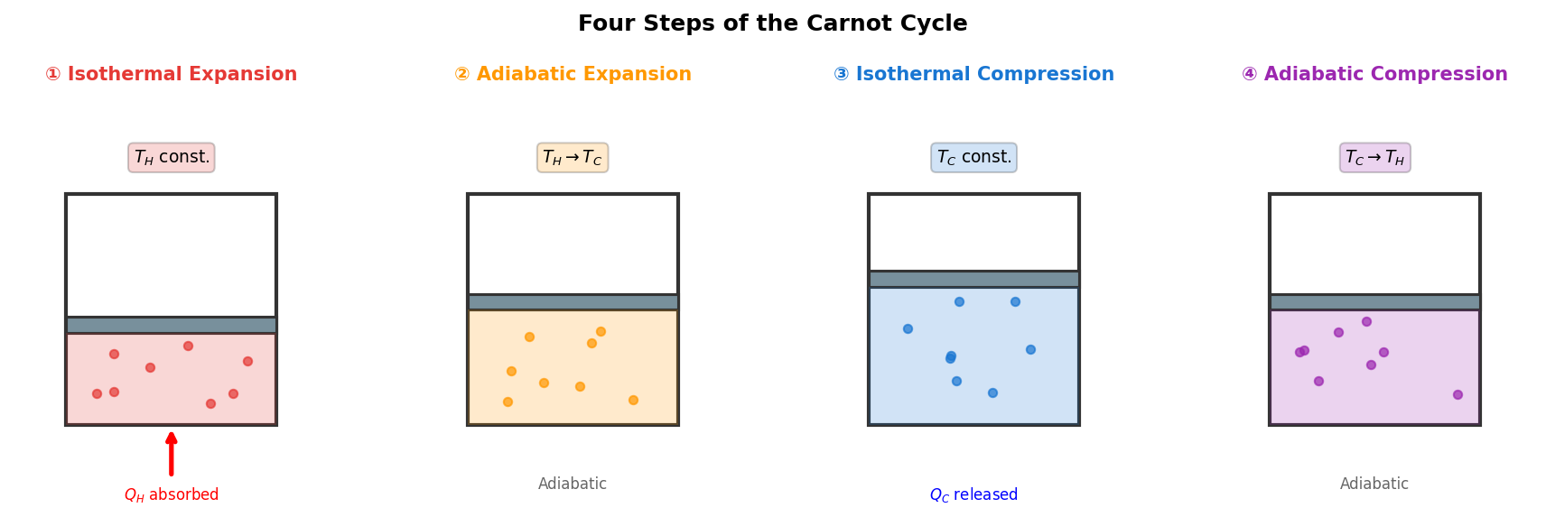
Fig. 3.2: The 4 steps of the Carnot cycle. Each step is physically illustrated with a cylinder and piston. ① Absorbing heat \(Q_H\) from the hot source and expanding, ② Adiabatic expansion causing temperature drop, ③ Releasing heat \(Q_C\) to the cold source and compressing, ④ Adiabatic compression restoring temperature.
🟡 Lina: When you plot these 4 steps on a pressure-volume diagram (PV diagram), it looks like Fig. 3.3 "PV diagram of the Carnot cycle".
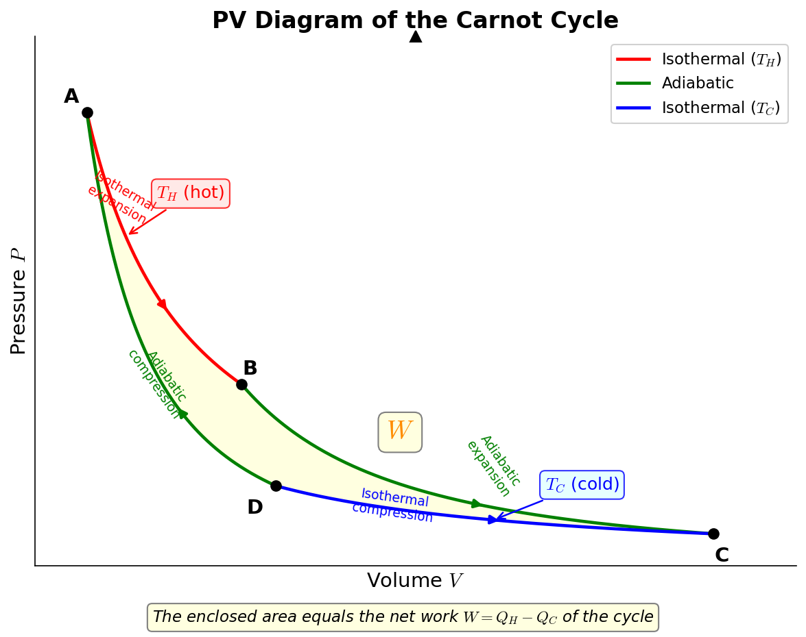
Fig. 3.3: PV diagram of the Carnot cycle. The 4 steps of the Carnot cycle (isothermal expansion → adiabatic expansion → isothermal compression → adiabatic compression) shown on a pressure-volume diagram. The enclosed area corresponds to the net work \(W\).
🟡 Lina: After going through the 4 steps, the gas returns to its original state—that's why it's called a "cycle."
🔵 Kai: If it returns to the original state... does the internal energy also return to its original value?
🟡 Lina: Exactly. If the state returns to the original, the change in internal energy is zero. From energy conservation:
That is, the work equals the "absorbed heat" minus the "discharged heat."
🔵 Kai: I see, only the net difference becomes work. But if we could make \(Q_C\) zero, couldn't we convert everything to work...?
Definition of Efficiency and Carnot's Conclusion
🟡 Lina: Efficiency \(\eta\) is defined as "what fraction of the input heat is converted to work":
🔵 Kai: To get 100% efficiency, we'd need \(Q_C = 0\), meaning zero waste heat? But is there a physical reason why waste heat can't be zero?
🟡 Lina: That's exactly the crux. Carnot showed that for a reversible cycle, \(Q_H/T_H = Q_C/T_C\) holds—meaning if \(T_C > 0\), then necessarily \(Q_C > 0\), and waste heat cannot be zero.
🔵 Kai: Wait, why does \(Q_H/T_H = Q_C/T_C\) hold? Dividing by temperature makes them equal—that's not intuitive at all.
🟡 Lina: Good question. I'll derive it explicitly now.
Derivation of the Carnot Efficiency
🟡 Lina: Using an ideal gas as the working substance, we can calculate each step explicitly. The ideal gas equation of state is \(pV = Nk_B T\). In high school you might have learned \(pV = nRT\) (\(n\) is the amount of substance, \(R\) is the gas constant), but rewriting in terms of \(N\) molecules gives \(Nk_B = nR\), so it's the same equation. Here \(k_B \approx 1.381 \times 10^{-23}\;\text{J/K}\) is the Boltzmann constant—a conversion factor that connects energy and temperature at the single-molecule level. It's related to the gas constant \(R\) you learned in high school by \(R = N_A k_B\) (\(N_A\) is Avogadro's number). In this chapter, writing in terms of the number of molecules \(N\) makes it easier to connect to statistical mechanics later.
Step 1 (Isothermal expansion \(A \to B\), temperature \(T_H\)):
First, internal energy is the total energy possessed by all particles constituting the system—the sum of all kinetic energies of the particles and the potential energies of their interactions. For an ideal gas, there are no forces between particles, so the potential energy is zero, and the internal energy is entirely kinetic energy—determined only by the speeds of the particles. In an isothermal process, temperature is constant, so the average speed of particles is also constant—therefore the internal energy doesn't change either.
🔵 Kai: I see, if the temperature doesn't change, the particle motion doesn't change either, so the internal energy stays constant.
🟡 Lina: Exactly. Next, we use energy conservation. The heat added to the system is distributed between the increase in internal energy and the work done by the system—that is, "heat added = change in internal energy + work done." In equation form:
Here \(dU\) is the infinitesimal change in internal energy, \(\delta Q\) is the infinitesimal heat added, and \(p\,dV\) is the infinitesimal work done by the system when the volume changes by \(dV\). You might notice the different symbols \(\delta\) and \(d\)—for now, think of both as "symbols representing infinitesimal quantities." The reason for the distinction is explained in "First Law (Energy Conservation)". This is energy conservation itself, and in a later section we'll formally name it the First Law.
For now, remember "heat added = change in internal energy + work done." In an isothermal process, the change in internal energy is zero, so \(\delta Q = p\,dV\). That is, the absorbed heat equals \(\delta Q = p\,dV\) summed up (integrated) over the entire process. Substituting \(p = Nk_BT_H/V\) from the equation of state \(pV = Nk_BT_H\):
Here we used \(\int_{V_A}^{V_B} \frac{dV}{V} = [\ln V]_{V_A}^{V_B} = \ln V_B - \ln V_A = \ln\frac{V_B}{V_A}\). You learned \(\int 1/x\,dx = \ln x\) in high school.
⚪ Mei: So the absorbed heat is determined by the temperature and the logarithm of the volume ratio. The more the gas expands, the more heat it absorbs.
Step 3 (Isothermal compression \(C \to D\), temperature \(T_C\)):
🟡 Lina: Since it's an isothermal process, just like in Step 1, the change in internal energy is zero and \(\delta Q = p\,dV\) holds. But this time the temperature is \(T_C\), so the equation of state gives \(p = Nk_BT_C/V\). In Step 1, it was expansion (\(dV > 0\)) so \(\delta Q > 0\)—the system was absorbing heat. This time it's compression, so \(dV < 0\)—meaning \(p\,dV < 0\), and \(\delta Q = p\,dV < 0\). Since \(\delta Q\) is "heat added to the system," a negative value means "heat left the system"—the system is releasing heat. The total heat added to the system over the entire process is found by integrating as the volume changes from \(V_C\) to \(V_D\) (since it's compression, \(V_D < V_C\)):
Mechanically computing \(\int_{V_C}^{V_D} \frac{dV}{V} = [\ln V]_{V_C}^{V_D} = \ln V_D - \ln V_C = \ln(V_D/V_C)\) gives the correct result.
Since \(V_D < V_C\) (volume decreases due to compression), \(\ln(V_D/V_C) < 0\)—so the integral result \(Nk_B T_C \ln(V_D/V_C)\) is negative. Indeed, the system is releasing heat.
Here we want to define \(Q_C\) as "the magnitude of heat released by the system to the cold source" as a positive value. Since the integral result is negative (representing "the system lost heat"), we take its absolute value:
The last equality uses \(-\ln(a/b) = \ln(b/a)\).
🔵 Kai: How do the two adiabatic processes come in?
🟡 Lina: In adiabatic processes, \(\delta Q = 0\), so the First Law becomes \(dU = -p\,dV\). For a monatomic ideal gas (a gas of single atoms like helium), particles only move in the \(x\), \(y\), \(z\) directions, and it's experimentally known that each direction carries \(\frac{1}{2}k_BT\) of energy (\(k_B\) is the Boltzmann constant that appeared earlier in the equation of state). That means \(\frac{3}{2}k_BT\) per particle, and \(U = \frac{3}{2}Nk_BT\) for \(N\) particles. Why this holds will be derived from statistical mechanics later in this chapter (3.7 "The Statistical Mechanical Meaning of Temperature"). For now, please accept it as an experimental fact. The infinitesimal change is \(dU = \frac{3}{2} N k_B\,dT\). Combining this with the equation of state \(p = Nk_BT/V\), let's derive how temperature and volume are related in an adiabatic process. Substituting into \(dU = -p\,dV\):
Dividing both sides by \(Nk_B T\) gives \(\frac{3}{2}\frac{dT}{T} = -\frac{dV}{V}\). Notice that the left side is a function of \(T\) only and the right side is a function of \(V\) only. When this happens, you can integrate each side with respect to its own variable (a technique called separation of variables). Using \(\int dT/T = \ln T\) and \(\int dV/V = \ln V\), we get \(\frac{3}{2}\ln T = -\ln V + \text{const}\). Moving \(\ln V\) to the left: \(\frac{3}{2}\ln T + \ln V = \text{const}\). Using logarithm properties \(a\ln x = \ln x^a\) and \(\ln x + \ln y = \ln(xy)\): \(\ln(T^{3/2} V) = \text{const}\). Taking the exponential of both sides: \(T^{3/2} V = \text{constant}\).
🔵 Kai: Oh, so temperature and volume are linked together. If it expands, the temperature drops.
🟡 Lina: Right. We could use it as is, but to make the "\(T\) and \(V\) relationship" easier to see, I want to make the exponent on \(T\) equal to 1, so I'll raise both sides to the \(2/3\) power. \((T^{3/2} V)^{2/3} = T^{(3/2)(2/3)} \cdot V^{2/3} = T \cdot V^{2/3}\), so we can write \(T V^{2/3} = \text{constant}\) (the specific value of the constant on the right changes, but "constant" is the same). In high school you might have learned \(pV^\gamma = \text{constant}\) (\(\gamma\) is the heat capacity ratio); for a monatomic ideal gas \(\gamma = 5/3\), giving \(TV^{\gamma-1} = TV^{2/3} = \text{constant}\), the same equation. The important point is that "in an adiabatic process, temperature and volume cannot change independently." Applying this to the adiabatic expansion \(B \to C\) and adiabatic compression \(D \to A\):
Let's try dividing the first equation by the second. The left side is \(\frac{T_H V_B^{2/3}}{T_C V_D^{2/3}}\), the right side is \(\frac{T_C V_C^{2/3}}{T_H V_A^{2/3}}\)—hmm, that's a bit complicated. Let me do it more simply. From the first equation: \(V_B^{2/3} = (T_C/T_H) V_C^{2/3}\). From the second equation: \(V_A^{2/3} = (T_C/T_H) V_D^{2/3}\). Dividing these two, \(T_C/T_H\) cancels:
Removing the \(2/3\) power (raising both sides to the \(3/2\) power):
🔵 Kai: Ah, the arguments inside the logarithms become the same! So if we take the ratio \(Q_C/Q_H\)... the logarithms cancel, don't they?
🟡 Lina: Exactly. Since \(\ln(V_B/V_A) = \ln(V_C/V_D)\), taking the ratio of \(Q_H\) and \(Q_C\) causes the logarithmic factors to cancel, leaving only the ratio of temperatures:
Therefore, the efficiency of the Carnot cycle is:
🔵 Kai: But we calculated this using a monatomic ideal gas, right? Wouldn't it be different for other gases?
🟡 Lina: Good question. Actually, the Carnot efficiency is independent of the working substance. Here we calculated it explicitly for a monatomic ideal gas, but whether you use diatomic molecules or a liquid, any reversible cycle gives the same result. This is a consequence of Carnot's theorem—if the efficiency depended on the working substance, you could combine the more efficient one with the less efficient one to create a device that violates the Second Law.
⚪ Mei: So unless the cold source temperature is zero, the efficiency can never reach 100%.
🟡 Lina: What's even more important is Carnot's theorem—among all heat engines operating between the same temperatures, the reversible engine (Carnot engine) has the maximum efficiency. Any irreversible engine necessarily achieves lower efficiency.
🔵 Kai: Why?
🟡 Lina: If there were an engine more efficient than the Carnot engine, you could combine it with a reversed Carnot engine (heat pump) to "transfer heat from the cold source to the hot source with no cost whatsoever." This contradicts the Second Law, which we'll discuss shortly.
📝 Exercises:
- Concrete calculation of Carnot efficiency → Problem B-1. Calculating Carnot Efficiency
✅ Comprehension Check: Write the formula for the upper limit of Carnot cycle efficiency.
Answer
\(\eta_{\text{Carnot}} = 1 - \frac{T_C}{T_H}\)
✅ Comprehension Check: Under what conditions does the Carnot efficiency limit fail to reach 100%?
Answer
As long as the cold source temperature \(T_C\) is not zero, the efficiency cannot reach 100%.
3.3 The Laws of Thermodynamics — Energy Conservation and Directionality
🟡 Lina: Building on Carnot's work, the laws of thermodynamics were formalized in the 19th century. There are laws from the Zeroth to the Third, but the most important are the Zeroth, First, and Second Laws.
Zeroth Law (Transitivity of Thermal Equilibrium)
🟡 Lina: The Zeroth Law is the law that guarantees the existence of temperature.
If system \(A\) is in thermal equilibrium with system \(C\), and system \(B\) is also in thermal equilibrium with system \(C\), then system \(A\) and system \(B\) are in thermal equilibrium with each other.
⚪ Mei: That sounds obvious...
🟡 Lina: It "seems" obvious, but it's precisely because this transitivity holds that we can label all systems with a single number called "temperature." If this law didn't hold, situations like "\(A\) and \(C\) are in equilibrium but \(A\) and \(B\) are not" could occur, and the concept of temperature itself would become meaningless.
✅ Comprehension Check: Why is the Zeroth Law of thermodynamics important? What would go wrong if it didn't hold?
Answer
Because the Zeroth Law (transitivity of thermal equilibrium) holds, all systems can be labeled with a single number called "temperature." If it didn't hold, the concept of temperature itself would become meaningless.
First Law (Energy Conservation)
🟡 Lina: The First Law is energy conservation. Written in differential form:
Here \(dU\) is the change in internal energy, \(\delta Q\) is the heat added to the system, and \(\delta W\) is the work done by the system. If we consider gas expansion/compression, \(\delta W = p\,dV\), so:
This is exactly the same equation as "heat added = change in internal energy + work done" (\(\delta Q = dU + p\,dV\)) that we used in the Carnot cycle derivation, just solved for \(dU\).
🔵 Kai: Why are \(d\) and \(\delta\) different?
🟡 Lina: Good question. \(dU\) is an infinitesimal change of a state variable—once the state of the system is determined, the value of \(U\) is uniquely determined. On the other hand, \(\delta Q\) and \(\delta W\) are path-dependent quantities—their values depend on what process was followed. It's like the difference between your bank account balance (state variable) and the amount of cash deposited (path-dependent).
⚪ Mei: Let me organize this.
Table 3.1: Comparison of state variables and path-dependent quantities
| Category | Notation | Examples | Characteristics |
|---|---|---|---|
| State variables (\(d\)) | \(dU\), \(dS\), \(dV\) | Internal energy, entropy, volume | Uniquely determined once the state is specified. Path-independent |
| Path-dependent quantities (\(\delta\)) | \(\delta Q\), \(\delta W\) | Heat, work | Values change depending on the process taken |
✅ Comprehension Check: In the First Law equation \(dU = \delta Q - \delta W\), why are the symbols \(d\) and \(\delta\) used differently?
Answer
\(dU\) represents the infinitesimal change of a state variable (a quantity uniquely determined once the system's state is specified), while \(\delta Q\) and \(\delta W\) represent path-dependent quantities (quantities whose values change depending on the process taken).
Second Law (Entropy Increase / Irreversibility)
🟡 Lina: The Second Law is the law of "directionality." There are several equivalent formulations:
Clausius's statement: Heat does not spontaneously flow from a cold body to a hot body.
Kelvin's statement: There is no process whose sole result is to extract heat from a heat source and convert it entirely into work.
🔵 Kai: Isn't that obvious? Hot coffee cools down, but cold coffee never spontaneously heats up.
🟡 Lina: It "seems" obvious, right? But this is actually a deep mystery. Newton's equation \(F = ma\) is time-reversal symmetric—meaning the form of the equation doesn't change if you reverse time. The motion of microscopic particles is consistent with the laws of physics whether played forward or backward.
🔵 Kai: Wait a moment. If microscopic laws are time-reversal symmetric... does that mean a process where "heat flows from cold to hot" is also allowed microscopically? But isn't that a contradiction? It's OK microscopically but never happens macroscopically? So the Second Law isn't an "absolute law" like Newton's laws?
🟡 Lina: Good intuition. Actually, that's right—the character of the Second Law is fundamentally different from Newton's equation of motion. The person who resolved this contradiction was Boltzmann—but before that, let's look at the thermodynamic definition of entropy.
✅ Comprehension Check: Write the First Law in differential form.
Answer
\(dU = \delta Q - p\,dV\) (the heat added to the system equals, by energy conservation, the sum of the change in internal energy and the work done by the system).
✅ Comprehension Check: What is the Clausius statement of the Second Law of thermodynamics?
Answer
Heat does not spontaneously flow from a cold body to a hot body.
3.4 The Thermodynamic Definition of Entropy
🟡 Lina: From the results of the Carnot cycle, something remarkable can be derived. For a reversible cycle:
Let me tidy up the notation a bit. Until now we've treated both \(Q_H\) and \(Q_C\) as positive values representing "magnitudes of heat." But to generalize from here, I'll switch to the sign convention where heat received by the system is positive, heat released by the system is negative. Under this convention, the heat released during isothermal compression is written as \(-Q_C\). Then the equation above becomes:
🔵 Kai: Going around once and summing gives zero... is that a coincidence?
🟡 Lina: It's not a coincidence. This can actually be generalized. The Carnot cycle is a special closed curve, but I want to show that the same thing holds for any reversible cycle of arbitrary shape. Consider drawing an arbitrary closed curve on a PV diagram and dividing its interior into a fine grid. The reason a grid can be constructed is that through each point on the PV diagram, you can draw exactly one "constant-temperature curve (isotherm)" and one "no-heat-exchange curve (adiabat)." An isotherm is "the set of \((p, V)\) satisfying the equation of state \(pV = Nk_BT\) for a fixed \(T\)," so one exists for each temperature. Similarly, an adiabat passes through each point as the curve satisfying "\(TV^{2/3} = \text{constant}\)." It's just like how exactly one "meridian" and one "parallel" pass through every point on a map.
🔵 Kai: Ah, like meridians and parallels on a map, isotherms and adiabats cross everywhere on the PV diagram to form a grid.
🟡 Lina: Exactly. Using isotherms and adiabats as grid lines, you can divide the PV diagram into fine cells. Each cell has 4 sides: "isotherm → adiabat → isotherm → adiabat"—in other words, each cell is a tiny Carnot cycle. The relation \(Q_H/T_H = Q_C/T_C\) that we showed for an ideal gas is actually independent of the working substance by Carnot's theorem—it holds for any substance in a reversible Carnot cycle (if there were a substance for which it didn't hold, you could combine it with an ideal gas to create a device violating the Second Law). Therefore, for each tiny Carnot cycle, \(\delta Q_H/T_H + \delta Q_C/T_C = 0\) holds. If you fill the interior of any closed curve with these cells, you can approximate the curve as a collection of tiny Carnot cycles—like approximating a curve with a staircase.
🔵 Kai: The part about shared edges of adjacent cycles canceling each other is a bit hard to visualize...
🟡 Lina: Think of it this way. Imagine tiling a floor. When you cover the entire floor with small square tiles, the boundary between adjacent tiles is shared by two tiles. From one tile's perspective it's the "right edge," but from the neighboring tile's perspective it's the "left edge"—the same edge is traversed in opposite directions.
Physically, the isothermal expansion edge of one tiny cycle becomes the isothermal compression edge of the neighboring cycle. They traverse the same segment of the same isotherm, one in the expansion direction (\(\delta Q > 0\)) and the other in the compression direction (\(\delta Q < 0\)). Since the temperature is the same and the magnitudes of the changes are equal, the \(\delta Q/T\) contributions cancel exactly.
🔵 Kai: Ah, so adding the edges of neighboring cycles gives \(+\delta Q/T + (-\delta Q/T) = 0\).
🟡 Lina: Exactly. And what about the adiabatic edges? Remember that "adiabatic" means "no heat exchange" (we confirmed this in Steps 2 and 4). So on adiabatic lines, \(\delta Q = 0\), meaning \(\delta Q/T = 0\)—they don't contribute. In the end, all internal edges either "cancel with their neighbors on isotherms" or "are zero on adiabats," and only the outer boundary edges remain without cancellation.
🔵 Kai: Ah, the tile analogy makes sense! Everything internal cancels, leaving only the perimeter. ...But does this hold even if the perimeter is all squiggly?
🟡 Lina: Exactly. Since each tiny Carnot cycle satisfies \(\delta Q_H/T_H + \delta Q_C/T_C = 0\), summing over all of them leaves only the integral along the perimeter:
This means that "\(\delta Q_{\text{rev}}/T\) behaves like an exact differential."
🔵 Kai: What's an exact differential?
🟡 Lina: Let me use a mountain-climbing analogy. The elevation difference depends only on the starting and ending points—no matter which trail you take, \(h(B) - h(A)\) is the same value. This kind of "infinitesimal change that doesn't depend on the path" is called an exact differential. Mathematically, it means "there exists a function \(S\) such that the quantity can be written as its infinitesimal change \(dS\)." On the other hand, the distance walked depends on the path—this is an inexact differential. \(\delta Q\) is exactly like this: even with the same starting and ending points, its value changes depending on the intermediate process.
⚪ Mei: So \(\delta Q\) itself is like "distance walked" and path-dependent, but dividing by \(T\) makes it like "elevation difference"—path-independent.
🟡 Lina: Nice analogy. The fact that \(\oint \delta Q_{\text{rev}}/T = 0\) holds means that summing \(\delta Q_{\text{rev}}/T\) from \(A\) to \(B\) gives a result that doesn't depend on the path. Let me explain intuitively why. If there are two paths from \(A\) to \(B\), path I and path II, and the results were different—going via path I and returning via the reverse of path II would give a non-zero value for one complete loop. But that contradicts \(\oint = 0\). So any path must give the same value. I'll prove this rigorously in the next subsection. This means there exists a function \(S\) such that \(dS = \delta Q_{\text{rev}}/T\)—\(\delta Q_{\text{rev}}/T\) is an exact differential.
Remember—\(\delta Q\) itself was an inexact differential that depends on the path. But dividing by \(T\) transforms it into a path-independent quantity. In mathematics, a quantity that "converts an inexact differential into an exact differential by dividing" is called an integrating factor. Here, \(1/T\) plays the role of the integrating factor.
✅ Comprehension Check: \(\delta Q\) is a path-dependent quantity, but what property does \(\delta Q_{\text{rev}}/T\) have?
Answer
The integral of \(\delta Q_{\text{rev}}/T\) along a reversible process is path-independent (it behaves like an exact differential). This allows us to define entropy \(S\) as a state variable.
Entropy as a State Function
🟡 Lina: The fact that the loop integral over a reversible cycle is zero means that \(\int \delta Q_{\text{rev}}/T\) along a reversible process is path-independent.
Let's prove it. Consider two different reversible paths I and II going from state \(A\) to state \(B\). Consider the cycle "path I from \(A \to B\), then reverse of path II from \(B \to A\)":
Therefore:
🔵 Kai: Oh, you get the same value no matter which path you take! That's why it can be called a "state function."
🟡 Lina: Since it's path-independent, this defines a state function. Fixing a reference state \(O\):
Written in differential form:
This is the thermodynamic definition of entropy \(S\). \(\delta Q\) was an inexact differential that depends on the path, but dividing by \(T\) transforms it into a path-independent state function. \(T\) plays the role of an integrating factor.
The Fundamental Relation of Thermodynamics
🟡 Lina: Substituting \(\delta Q_{\text{rev}} = T\,dS\) into the First Law:
This is the fundamental relation of thermodynamics. \(dU\), \(dS\), and \(dV\) are all total differentials of state functions—no inexact differentials are involved.
🔵 Kai: That's elegant. But can this equation only be used for reversible processes?
🟡 Lina: Good question. Since \(U\), \(S\), and \(V\) are all state functions, this equation holds as a relation between any equilibrium states. It can be used universally as an expression relating the differences between two equilibrium states, regardless of whether the process is reversible or irreversible.
Verification with the Carnot Cycle
🟡 Lina: Let's verify the entropy changes in the Carnot cycle.
- Isothermal expansion (\(T_H\)): \(\Delta S_1 = Q_H / T_H\)
- Adiabatic expansion: \(\Delta S_2 = 0\) (since \(\delta Q = 0\))
- Isothermal compression (\(T_C\)): \(\Delta S_3 = -Q_C / T_C\)
- Adiabatic compression: \(\Delta S_4 = 0\)
Change over one cycle:
⚪ Mei: Indeed zero. Since entropy is a state function, it returns to its original value after one cycle.
🔵 Kai: But what if the process is irreversible? Does it not return to zero after one cycle?
🟡 Lina: Good question. For irreversible processes, \(\delta Q/T < dS\), that is:
Equality holds for reversible processes. For an adiabatic system (\(\delta Q = 0\)):
This is the law of entropy increase—the Second Law expressed in terms of entropy.
✅ Comprehension Check: Write the thermodynamic definition of entropy in differential form.
Answer
\(dS = \delta Q_{\text{rev}} / T\) (the infinitesimal heat added to the system in a reversible process, divided by temperature).
3.5 Boltzmann's Entropy — From Micro to Macro
🟡 Lina: The thermodynamics we've covered so far uses no information about the microscopic world. "Heat," "temperature," and "entropy" have all been defined as macroscopic quantities. Boltzmann's idea was revolutionary—macroscopic thermal phenomena can be explained by the statistical behavior of microscopic particles.
Microstates and Macrostates
🔵 Kai: Statistical?
🟡 Lina: For example, think about the air in a room. There are about \(10^{23}\) air molecules. Tracking the motion of each one is impossible. But "how the whole thing behaves" can be predicted using probability and statistics.
Let me distinguish two concepts here.
- Macrostate: A state specified by macroscopically measurable quantities such as temperature, pressure, and volume
- Microstate: A state where the positions and velocities (or quantum states in quantum mechanics) of all particles are completely specified
For a given macrostate, there are generally an enormous number of corresponding microstates.
🔵 Kai: So even though you can't know how a single molecule moves, you can make predictions when you look at \(10^{23}\) of them together?
🟡 Lina: Exactly. You can't predict the result of rolling a die once, but if you roll it a million times, you can predict that each face appears roughly equally. Same principle.
Boltzmann's Entropy
🟡 Lina: Boltzmann defined entropy as follows:
Where: - \(\Omega\) = the number of microstates corresponding to a given macrostate - \(k_B \approx 1.381 \times 10^{-23}\;\text{J/K}\) = Boltzmann constant. As you can tell from the units J/K (energy ÷ temperature), it serves as a conversion factor connecting the microscopic world (energy) to the macroscopic world (temperature) - \(\ln\) = natural logarithm
🔵 Kai: Why take the logarithm?
🟡 Lina: For additivity. When you place two independent systems side by side, the number of microstates of the combined system is a product:
Why a product? Because for every microstate of system 1, all microstates of system 2 are possible. It's the same reason two dice give \(6 \times 6 = 36\) combinations.
Taking the logarithm converts the product into a sum:
Entropy becomes an additive quantity. The same property as energy or volume.
⚪ Mei: So taking the logarithm is for "converting multiplication to addition." It comes from a physical requirement, not a mathematical trick.
Understanding with a Coin Example
🟡 Lina: Let's think with a concrete example. Flip 4 coins.
Table 3.2: Macrostates and entropy for 4 coins
| Macrostate (number of heads) | Number of microstates \(\Omega\) | Entropy \(S/k_B = \ln\Omega\) |
|---|---|---|
| 0 (all tails) | 1 | 0 |
| 1 | 4 | 1.39 |
| 2 | 6 | 1.79 |
| 3 | 4 | 1.39 |
| 4 (all heads) | 1 | 0 |
🔵 Kai: All heads or all tails has only 1 way, but half-and-half has 6 ways!
⚪ Mei: So "2 heads and 2 tails" has the largest \(\Omega\) and maximum entropy.
🟡 Lina: Right. It's obvious at a glance when you graph it (Fig. 3.4 "Number of microstates and entropy for coins"). See how the middle peaks?
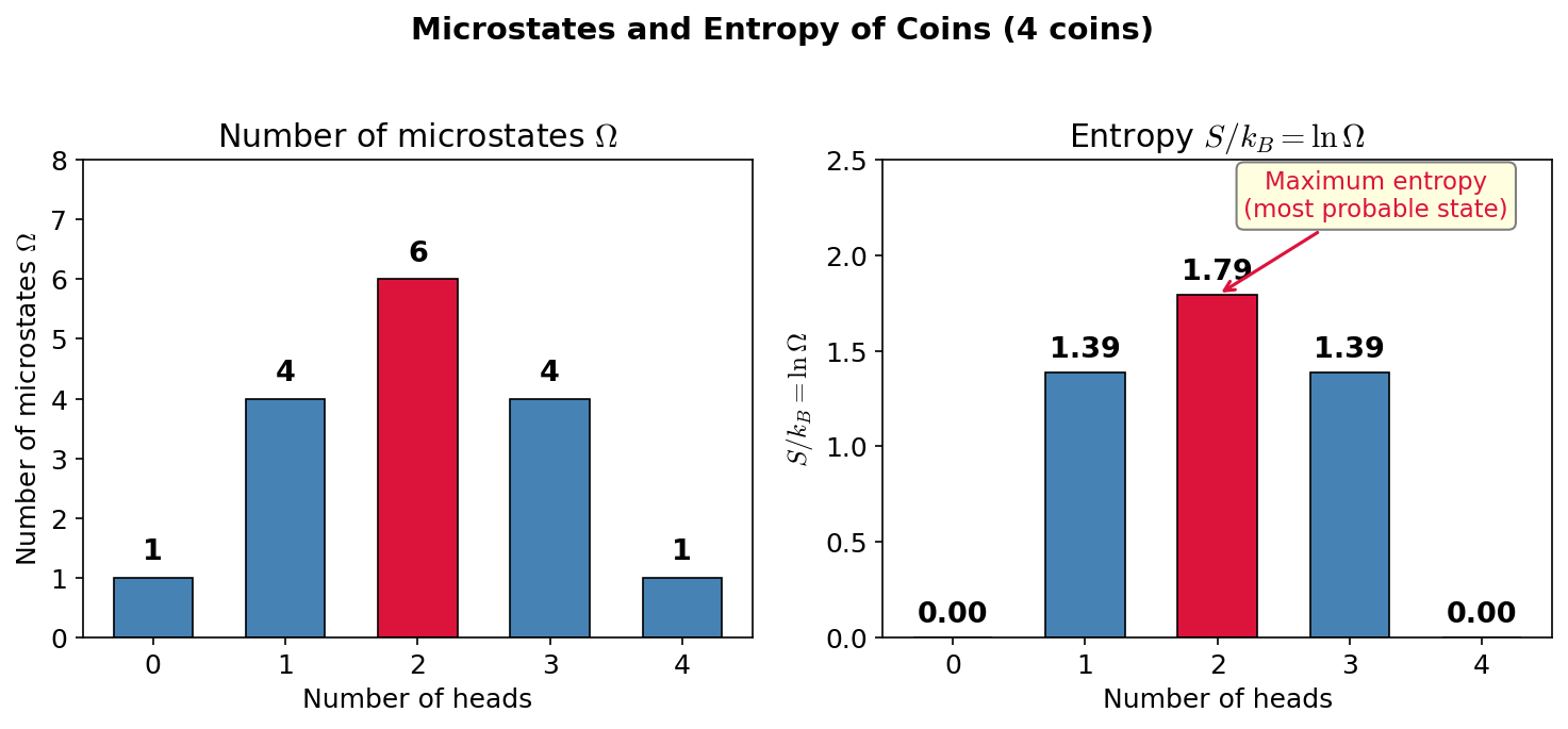
Fig. 3.4: Number of microstates and entropy for coins. For 4 coins, the number of microstates \(\Omega\) and entropy \(S/k_B = \ln\Omega\) for each macrostate (number of heads). Entropy is maximized at the most uniform distribution (2 heads).
✅ Comprehension Check: In the 4-coin example, which macrostate has maximum entropy? Why?
Answer
The macrostate with 2 heads and 2 tails. Because the number of corresponding microstates \(\Omega = 6\) is the largest (\(S = k_B \ln \Omega\) is maximized).
🟡 Lina: Right. And with \(10^{23}\) particles, the \(\Omega\) of "uniformly distributed states" is overwhelmingly larger than the \(\Omega\) of "states concentrated in one place." So the system naturally moves toward states with larger \(\Omega\)—that is, higher entropy. Look at Fig. 3.5 "Free expansion and entropy increase" for a concrete image. When you remove the partition in a box, the gas spontaneously spreads throughout. Focusing only on "which half each particle is in," the initial state (all particles in the left half) has only 1 configuration, but at equilibrium, each particle can be in either half, so the number of configurations explosively increases to \(2^N\).
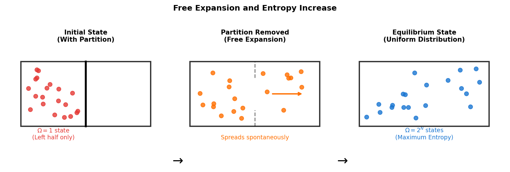
Fig. 3.5: Free expansion and entropy increase. When the partition is removed, the gas spontaneously spreads throughout. Focusing only on "which half each particle is in," the initial state (all particles in the left half) has only 1 configuration, but at equilibrium (uniform distribution), each particle can be in either half, so the number of configurations increases to \(2^N\).
Why the Second Law Holds
🔵 Kai: That's why "heat flows from hot to cold"?
🟡 Lina: Yes. Heat flows from hot to cold because doing so increases the total number of microstates \(\Omega\). It's not forbidden—the probability of it happening in reverse is just astronomically small.
🔵 Kai: So it's not "forbidden" but "almost certainly happens that way"... But how small is "almost certainly"? Like winning the lottery? Or orders of magnitude smaller?
🟡 Lina: Let's estimate it concretely. If \(N\) gas molecules are in a box, the probability that all molecules gather in the left half is:
For \(N = 10^{23}\):
🔵 Kai: \(10^{-3 \times 10^{22}}\)... that's way beyond lottery odds. A probability with \(10^{22}\) zeros is basically "never happens."
🟡 Lina: Even if you tried once every second for the age of the universe (about \(10^{10}\) years \(\approx 10^{17}\) seconds), it would never happen once.
🔭 Philosophy of Science Note: The Second Law is not a "law that can never be violated" but a "statistical law whose probability of violation is astronomically small." This is fundamentally different in character from deterministic laws like Newton's equation of motion. Decide for yourself—can you confidently say "an event with probability \(10^{-10^{22}}\) will not occur"?
📝 Exercises:
- Number of microstates and entropy for coins → Problem M-1. Entropy of Coins
✅ Comprehension Check: Write Boltzmann's definition of entropy and state what \(\Omega\) represents.
Answer
\(S = k_B \ln \Omega\). \(\Omega\) is the number of microstates (the total number of microscopic configurations that yield the same macroscopic state).
✅ Comprehension Check: Explain why heat flows from hot to cold, using the number of microstates.
Answer
Heat flowing from hot to cold increases the total number of microstates \(\Omega\). It's not forbidden for it to flow in reverse—the probability is just astronomically small.
3.6 Number of Microstates for an Ideal Gas — A Concrete Calculation
🟡 Lina: Since \(S = k_B \ln \Omega\) might seem abstract, let's concretely calculate \(\Omega\) for an ideal gas.
Problem Setup
🟡 Lina: Consider \(N\) identical particles (mass \(m\)) confined in a box of volume \(V\) with total energy \(E\).
In classical mechanics, each particle's state is completely specified by 6 numbers: position \((x, y, z)\) and momentum \((p_x, p_y, p_z)\). Momentum is "mass × velocity," a vector quantity with components \(p_x = mv_x\), \(p_y = mv_y\), \(p_z = mv_z\) in each direction.
🔵 Kai: Isn't position alone sufficient?
🟡 Lina: No. Even at the same position, a fast-moving particle and a stationary particle are in different states. So you need both "where it is" and "how it's moving." For 1 particle, there are 6 numbers \((x, y, z, p_x, p_y, p_z)\)—if you think of these as 6 coordinate axes in a 6-dimensional space, a single point in that space completely represents "where the particle is and how it's moving." For 2 particles, \(6 \times 2 = 12\) numbers determine the entire system's state. For \(N\) particles, you need \(6N\) variables total. The \(6N\)-dimensional space with these \(6N\) variables as coordinate axes is called phase space. "Phase" here is unrelated to wave phase—there are various theories about the name's origin, but for now think of it as "the space that completely represents the system's state." A single point in phase space corresponds to one microstate of the entire system.
⚪ Mei: So for \(10^{23}\) particles, a single point in a \(6 \times 10^{23}\)-dimensional space completely describes the entire system. An enormous number of dimensions, but the concept is simple.
The Energy Constraint
🟡 Lina: In an ideal gas, there are no interactions between particles, so the total energy is the sum of kinetic energies:
To make the structure of this equation clearer, let's line up the \(3N\) momentum components as \(\xi_1, \xi_2, \ldots, \xi_{3N}\) (\(\xi_1 = p_{x,1}\), \(\xi_2 = p_{y,1}\), \(\xi_3 = p_{z,1}\), \(\xi_4 = p_{x,2}\), ...). Then the total energy condition becomes:
🔵 Kai: \(\xi_1^2 + \xi_2^2 + \cdots = 2mE\) looks like some kind of sphere? In 3 dimensions, \(x^2 + y^2 + z^2 = R^2\) is a sphere...
🟡 Lina: Good intuition. That's exactly right—this is the equation of a \(3N\)-dimensional sphere with radius \(\sqrt{2mE}\). So once the energy is fixed, the "distribution" of momenta is restricted to the surface of a sphere, and the larger the energy, the larger the sphere becomes, which increases the number of states. The energy constraint translates into a geometric constraint—the size of the sphere.
⚪ Mei: So the energy constraint gets converted into a geometric condition—the "radius of the sphere."
🟡 Lina: Right. I've drawn an illustration in Fig. 3.6 "Sphere in momentum space and number of microstates".
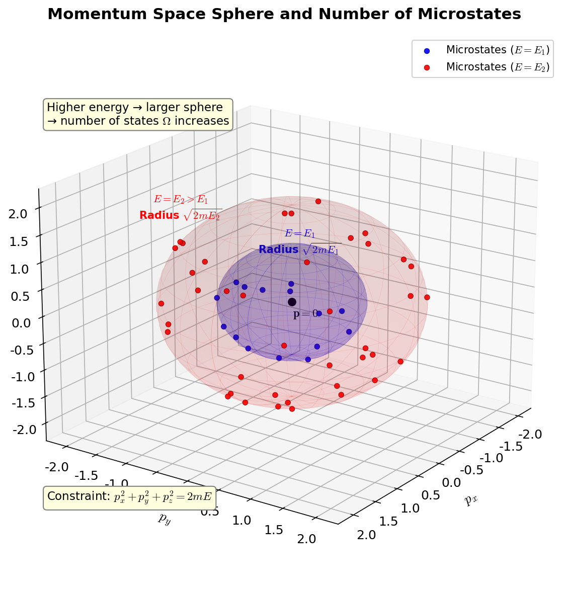
Fig. 3.6: Sphere in momentum space and number of microstates. The microstates of an ideal gas correspond to a sphere (its interior) of radius \(\sqrt{2mE}\) in momentum space. As energy increases, the sphere grows larger and the number of microstates increases.
The states with exactly energy \(E\) lie on the sphere's surface, but when counting microstates, we use the volume inside the sphere (all states with energy \(E\) or less). In high dimensions, most of the sphere's volume is actually concentrated near the surface. Intuitively, the volume of a \(d\)-dimensional sphere is proportional to \(R^d\), so the ratio of the volume of a sphere of radius \(0.99R\) to one of radius \(R\) is \((0.99)^d\)—for \(d = 3\) it's about 97%, but for \(d = 10^{23}\), \((0.99)^{10^{23}} \approx 0\), meaning almost all the volume is concentrated in the outer 1% shell. So whether you count using the interior volume or the surface area of the shell, the result is the same. Here we'll proceed by taking it as proportional to the interior volume.
🔵 Kai: In high dimensions, volume concentrates at the surface... that's counterintuitive. But when you say \((0.99)^{10^{23}} \approx 0\), it makes sense.
Volume of a \(3N\)-Dimensional Sphere
🔵 Kai: How do you find the volume of a \(3N\)-dimensional sphere? For 3 dimensions it's \(\frac{4}{3}\pi R^3\), but...
🟡 Lina: Good question. To find the number of microstates, we need to calculate the volume of a sphere of radius \(\sqrt{2mE}\) in momentum space. In 3 dimensions, the sphere volume is \(\frac{4}{3}\pi R^3\)—proportional to \(R^3\). Extending the same idea to \(d\) dimensions, using multiple integrals (I'll skip the derivation), you get:
Here \(\Gamma\) is the gamma function—a function that extends the factorial \(n!\) to non-integer values, satisfying \(\Gamma(n+1) = n!\) for integers \(n\). Why does \(\pi\) appear? Recall the area of a 2-dimensional circle \(\pi R^2\)—the \(\pi\) comes from "going all the way around in the angular direction." In higher dimensions it's the same: when computing the sphere volume with multiple integrals, integrating over all angular directions produces powers of \(\pi\), and integrating in the radial direction (distance from center) naturally produces factorials (or their generalization, the gamma function).
⚪ Mei: \(\pi\) comes from the "going all the way around" geometry, and \(\Gamma\) comes from "accumulating along the radial direction"—they arise from different origins.
🟡 Lina: Exactly. You don't need to memorize the formula—what matters is that it's proportional to \(R^d\). That means the higher the dimension \(d\), the more explosively the volume grows with even a small increase in radius \(R\). Let's verify with low dimensions. For \(d = 1\): \(V_1 = \frac{\pi^{1/2}}{\Gamma(3/2)} R = \frac{\sqrt{\pi}}{\frac{1}{2}\sqrt{\pi}} R = 2R\)—that's a line segment of length \(2R\), correct. For \(d = 2\): \(V_2 = \frac{\pi}{\Gamma(2)} R^2 = \pi R^2\)—area of a circle. For \(d = 3\): \(V_3 = \frac{\pi^{3/2}}{\Gamma(5/2)} R^3 = \frac{\pi^{3/2}}{\frac{3}{4}\sqrt{\pi}} R^3 = \frac{4}{3}\pi R^3\)—volume of a sphere. They all check out.
🔵 Kai: For \(\Gamma(d/2 + 1)\), if \(d\) is odd, you get things like \(\Gamma(3/2)\) or \(\Gamma(5/2)\)—non-integer arguments. Can those be computed?
🟡 Lina: Good point. The gamma function extends the factorial \(n!\) to non-integers and satisfies the recurrence relation \(\Gamma(n+1) = n \cdot \Gamma(n)\). The value \(\Gamma(1/2) = \sqrt{\pi}\) is known, and from there you can compute \(\Gamma(3/2) = \frac{1}{2}\sqrt{\pi}\), \(\Gamma(5/2) = \frac{3}{4}\sqrt{\pi}\), and so on. But what matters now isn't the details of these coefficients—it's that the volume is proportional to \(R^d\)—meaning the higher the dimension \(d\), the more explosively the volume grows with even a small increase in radius. We'll revisit the detailed properties of the gamma function when needed. Substituting \(R = \sqrt{2mE}\):
Assembling the Microstate Count
🟡 Lina: Next, let's consider the position degrees of freedom. A single particle can be anywhere within the volume \(V\), so the "number of choices" for position is proportional to \(V\). For 2 particles, particle 1 can be anywhere in \(V\) and particle 2 independently anywhere in \(V\)—so \(V \times V = V^2\). For \(N\) particles, \(V^N\). So the position degrees of freedom contribute a factor of \(V^N\).
🔵 Kai: Do you get the number of microstates by multiplying the momentum-space sphere volume by \(V^N\)?
🟡 Lina: A few more corrections are needed. First, the "volume" of phase space is continuous, so as-is it can't become a "count" of states—volume is a real-valued number, and you can't say "how many."
🔵 Kai: Right. If you're told "the area is 10 square meters," you can't say "how many squares" without specifying the square size.
🟡 Lina: Exactly. To count states, you need to divide phase space by some minimum unit to get "the number of cells." Just like deciding the cell size on graph paper. So what determines the cell size? This is where quantum mechanics (which we'll study in detail from the next chapter onward) enters. Quantum mechanics has a principle that "you cannot simultaneously determine position and momentum with perfect precision"—for example, trying to measure a particle's position precisely causes its momentum information to blur. As a consequence of this principle, phase space has a "minimum cell" smaller than which no distinction can be made. The constant that determines this minimum area is \(h\) (\(h \approx 6.626 \times 10^{-34}\;\text{J·s}\), called Planck's constant)—a fundamental constant by which nature has decided "I won't distinguish finer than this." Why this value and why such a principle exists will be studied in detail from the next chapter onward.
🔵 Kai: So the specific value of \(h\) is experimentally determined, and for now I should just accept it as "the cell size determined by nature"?
🟡 Lina: Exactly. In each direction, the minimum value of \(\Delta x \cdot \Delta p_x\) is of order \(h\). One particle has position and momentum in each of the \(x, y, z\) directions, so the minimum cell is \(h \times h \times h = h^3\) (it's a product because each direction is independent). For \(N\) particles, \(h^{3N}\). So we divide the phase space volume by \(h^{3N}\) to convert it to "number of states."
Furthermore, identical particles are indistinguishable when swapped—this is a requirement from quantum mechanics that we'll study in detail from the next chapter. Intuitively, you can't put "name tags" on helium atom A and helium atom B—they have exactly the same properties, so exchanging them is physically undetectable. For now, accept that "you cannot label identical particles to distinguish them." Swapping particle 1 and particle 2 gives the same microstate. There are \(N!\) permutations of \(N\) particles, so we divide by \(N!\) to remove duplicates. Putting it all together:
(When \(N\) is large, \(\Gamma(3N/2+1)\) can be handled with Stirling's approximation introduced in the next subsection, so you don't need to worry about whether the argument is an integer.)
🔵 Kai: That's complicated...
🟡 Lina: What matters is the dependence on \(E\) and \(V\). Viewing it as a function of \(E\) and \(V\) only with \(N\) fixed (all factors depending on \(N\) treated as constants):
⚪ Mei: Expanding the volume or increasing the energy—either one increases the number of microstates. A simple result, which is reassuring.
Entropy Calculation
🟡 Lina: Taking the logarithm:
As-is, \(\ln(N!)\) and \(\ln\Gamma(3N/2+1)\) are hard to handle. Here we use Stirling's approximation. When \(n\) is large, the logarithm of \(n!\) is:
This is because \(\ln n! = \ln 1 + \ln 2 + \cdots + \ln n\) can be approximated by the integral \(\int_1^n \ln x\,dx = n\ln n - n + 1 \approx n\ln n - n\).
🔵 Kai: It's convenient that the logarithm of a factorial can be approximated by \(n \ln n - n\). You certainly can't directly compute \(10^{23}!\).
🟡 Lina: Applying this: \(\ln(N!) \approx N\ln N - N\), \(\ln\Gamma(3N/2+1) \approx \frac{3N}{2}\ln\frac{3N}{2} - \frac{3N}{2}\). Simplifying: \(N\ln V - N\ln N = N\ln(V/N)\) and \(\frac{3N}{2}\ln(2mE) - \frac{3N}{2}\ln\frac{3N}{2} = \frac{3N}{2}\ln\frac{4mE}{3N}\). Further decomposing \(\ln\frac{4mE}{3N} = \ln\frac{E}{N} + \ln\frac{4m}{3}\), the \(\ln\frac{4m}{3}\) part is a constant independent of both \(E\) and \(V\), so it can be grouped with other constant terms involving \(m\) and \(h\) (noting that the argument of the logarithm becomes dimensionless when combined with these constants). The final result is called the Sackur-Tetrode formula:
Here (constant) contains all terms constructed from \(m\), \(h\), \(k_B\), etc. You might wonder "the argument of \(\ln(E/N)\) has dimensions of energy—is it okay to put that inside a logarithm?" In fact, the constant includes terms like \(\frac{3}{2}\ln(4\pi m / (3h^2))\) which, combined with the rest, make the logarithm's argument dimensionless. However, when taking partial derivatives with respect to \(E\) or \(V\), these constant terms vanish, so they don't affect the following calculations. So for now, it's fine to think "don't worry about the constant part."
⚪ Mei: The larger \(E\) is and the larger \(V\) is, the larger the entropy. Matches our intuition.
🟡 Lina: Right. More energy means a larger sphere in momentum space; more volume means a larger position space. Both increase the number of microstates.
✅ Comprehension Check: How does the number of microstates \(\Omega\) for an ideal gas depend on energy \(E\)?
Answer
\(\Omega \propto E^{3N/2}\). Because as energy increases, the volume of the sphere in momentum space increases.
3.7 The Statistical Mechanical Meaning of Temperature
🟡 Lina: Using Boltzmann's entropy, we can also give temperature a statistical mechanical meaning.
Derivation from the Thermal Equilibrium Condition of Two Systems
🟡 Lina: Consider two systems (system 1 and system 2) that can exchange energy. The total energy is conserved:
The number of microstates of the combined system is:
Here I'll make one important assumption. The principle of equal a priori probabilities—the assumption that for an isolated system, all microstates satisfying constraints like energy are realized with equal probability.
🔵 Kai: Why can we say they're equally probable?
🟡 Lina: A deep question. There's no rigorous proof. But the symmetry argument that "there's no reason to favor a particular microstate," combined with the fact that results derived from this assumption agree with experiment, supports this principle. Think of it as the starting assumption of statistical mechanics.
🔵 Kai: How does that lead to maximizing \(\Omega\)?
🟡 Lina: If each microstate is equally probable, then the probability of realizing a given macrostate is proportional to the number of microstates \(\Omega\) corresponding to that macrostate. So the macrostate with the largest \(\Omega\) is realized with the highest probability—meaning the system moves toward the energy distribution that maximizes \(\Omega_{\text{total}}\).
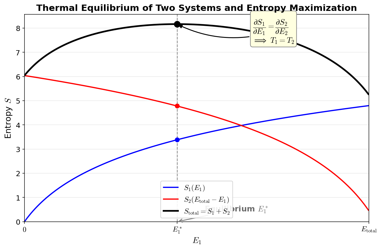
Fig. 3.7: Thermal equilibrium and entropy maximization. When two systems exchange energy, equilibrium is reached at the point where the total entropy \(S_{\text{total}} = S_1(E_1) + S_2(E_{\text{total}} - E_1)\) is maximized. At this point, \(\partial S_1/\partial E_1 = \partial S_2/\partial E_2\), i.e., \(T_1 = T_2\).
🟡 Lina: We just need to find the condition that maximizes \(\Omega_{\text{total}}\). I've drawn the concept in Fig. 3.7 "Thermal equilibrium and entropy maximization". Since it's easier to work with logarithms, let's write it in terms of entropy:
Differentiate with respect to \(E_1\) and set equal to zero:
Since \(E_2 = E_{\text{total}} - E_1\), we have \(\partial E_2 / \partial E_1 = -1\). Therefore:
🔵 Kai: At equilibrium, \(\partial S / \partial E\) is equal for both systems!
🟡 Lina: Right. And we know that "in thermal equilibrium, temperatures are equal." So \(\partial S / \partial E\) must be a quantity related to temperature. Indeed:
This is the statistical mechanical definition of temperature.
✅ Comprehension Check: Express the condition for two systems to reach thermal equilibrium through energy exchange, using entropy.
Answer
\(\frac{\partial S_1}{\partial E_1} = \frac{\partial S_2}{\partial E_2}\) (the energy derivatives of entropy are equal for both systems). This corresponds to the temperatures being equal.
Verification with an Ideal Gas
🟡 Lina: The entropy of an ideal gas we found earlier was \(S = k_B N \left[\frac{3}{2}\ln \frac{E}{N} + \ln\frac{V}{N} + (\text{constant})\right]\). When differentiating with respect to \(E\), since \(\ln(E/N) = \ln E - \ln N\), the \(\ln N\) part vanishes as a constant. Let's differentiate:
Rearranging:
🔵 Kai: \(E = \frac{3}{2}Nk_BT\)—that's the same equation we used in the adiabatic process calculation! The one we used without proof back then has now been derived?
🟡 Lina: Exactly. Earlier we used it as a "known fact," but now we've just derived it from statistical mechanics. The \(3\) is the number of degrees of freedom each particle has (motion in \(x\), \(y\), \(z\) directions), with \(\frac{1}{2}k_B T\) of energy per degree of freedom. This is called the equipartition theorem.
🔵 Kai: So if a molecule can also rotate, it gains more degrees of freedom, and at the same temperature it has more energy?
🟡 Lina: Exactly. A diatomic molecule gains 2 rotational degrees of freedom, giving \(E = \frac{5}{2}Nk_BT\). That's the power of the equipartition theorem. Moreover, starting from just the statistical mechanics definition \(1/T = \partial S/\partial E\), all these familiar formulas can be derived. Similarly, differentiating entropy with respect to \(V\) gives pressure:
Rearranging:
🔵 Kai: The ideal gas equation of state! But wait. When computing \(\partial S/\partial V\), you're holding \(E\) fixed, right? Why fix energy instead of temperature?
🟡 Lina: Good question. Here we're considering an isolated system (no energy exchange with the outside), so \(E\) is constant. Temperature is a quantity derived from \(E\), so at the starting point it's natural to hold \(E\) fixed.
⚪ Mei: So you find the entropy from \(S = k_B \ln \Omega\), differentiate with respect to \(E\) to get temperature, differentiate with respect to \(V\) to get pressure—everything comes out.
🟡 Lina: Exactly. Count the microstates, get the entropy, and just differentiate—temperature, pressure, equation of state all follow. All macroscopic quantities emerge from counting microstates—that's the power of statistical mechanics.
✅ Comprehension Check: When deriving \(E = \frac{3}{2}Nk_BT\) from the entropy of an ideal gas, what operation is performed?
Answer
Take the partial derivative of the entropy \(S = k_B N [\frac{3}{2}\ln E + \cdots]\) with respect to energy \(E\) to compute \(1/T = \partial S/\partial E\), then solve for \(E\).
The Intuitive Meaning of Temperature
🟡 Lina: Putting the definition \(1/T = \partial S / \partial E\) into words:
The lower the temperature of a system, the more the entropy (logarithm of the number of states) increases when a little energy is added.
A hot object is already "disordered," so adding energy doesn't open up that many new states. A cold object is still "orderly," so a little energy opens up many new states.
🔵 Kai: So lower temperature means more "room to grow." The effect of giving energy is larger.
🟡 Lina: Right. Let's confirm visually with the graph in Fig. 3.8 "Statistical mechanical meaning of temperature. The slope \(\partial S/\partial E = 1/T\) of the \(S\)-\(E\) graph gives the inverse of temperature. The steep region (blue) is low temperature". On an \(S\)-\(E\) graph, for the same system, in the low-energy region (low temperature) the slope \(\partial S/\partial E\) is steep, and in the high-energy region (high temperature) the slope becomes gentle.
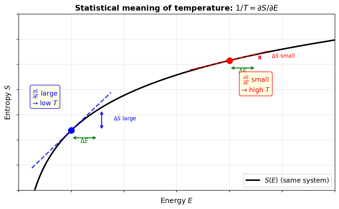
Fig. 3.8: Statistical mechanical meaning of temperature. The slope \(\partial S/\partial E = 1/T\) of the \(S\)-\(E\) graph gives the inverse of temperature. The steep region (blue) is low temperature—the same \(\Delta E\) produces a large entropy increase. The gentle region (red) is high temperature—adding energy barely increases entropy.
So when energy flows from the high-temperature system to the low-temperature system, the entropy decrease on the hot side is smaller than the entropy increase on the cold side, and overall entropy increases.
🔵 Kai: So that's why heat flows from hot to cold! But if the system is small—like only 10 particles—could you observe it flowing the other way?
🟡 Lina: Sharp. In fact, at the nanoscale, deviations from the Second Law are observed as "fluctuations." When the number of particles is small, the ratio of \(\Omega\) values isn't overwhelming. But for macroscopic systems (\(N \sim 10^{23}\)), it effectively never happens.
🔵 Kai: Huh, so the Second Law is an "approximate law" that holds because the number of particles is large.
🟡 Lina: Exactly. Newton's laws "hold deterministically for individual particles," but the Second Law is "a statistical law that effectively holds because \(N\) is large"—the character of the law is fundamentally different. There are at least two types of "ways physical laws hold"—deterministic laws that hold rigorously even for a single particle, and statistical laws that effectively hold only when \(N\) is large. The Second Law is the latter—violations are visible at the nanoscale but appear absolute at the macroscale.
⚪ Mei: So even though they're both "physical laws," the mechanisms by which they hold are completely different. Deterministic laws and statistical laws—we need to distinguish between them.
📝 Exercises:
- Deriving equality of temperatures from the thermal equilibrium condition → Problem M-2. Statistical Mechanical Definition of Temperature
✅ Comprehension Check: Write the statistical mechanical definition of temperature.
Answer
\(\frac{1}{T} = \frac{\partial S}{\partial E}\bigg|_{V,N}\) (the partial derivative of entropy with respect to energy is the inverse of temperature).
✅ Comprehension Check: When energy is added to a cold object, how does the number of microstates change?
Answer
It increases greatly (since \(\partial S / \partial E\) is large, \(T\) is small).
3.8 Free Energy \(F = U - TS\)
🟡 Lina: Let me introduce one more important concept. The Helmholtz free energy.
Motivation: Systems at Constant Temperature
🟡 Lina: In the laboratory, systems are often kept at constant temperature by contact with a large heat bath. In this case, the system's entropy is not constant (because it exchanges energy with the heat bath). Instead, the temperature \(T\) is constant.
In such situations, the quantity that determines "which state does the system settle into?" is the free energy:
The Minimization Principle for \(F\)
🟡 Lina: Considering the total system (system + heat bath), the total entropy increases (Second Law). Here we assume the system's volume is constant (no work is done)—a typical situation of a system in a container immersed in a heat bath. Under this condition, let's derive a condition written only in terms of the system's quantities, starting from the total system's entropy change.
🟡 Lina: Let's find the entropy change of the heat bath. Two key points:
- The heat bath is so large that receiving energy from the system barely changes its temperature. Imagine dropping a single drop of hot water into a huge pool—the pool's temperature hardly changes. So the heat bath is always approximately in equilibrium, and its energy exchange with the system is "just a tiny change" from the bath's perspective. Therefore, for the bath we can directly use \(dS = \delta Q_{\text{rev}}/T\)—for heat \(\Delta Q_{\text{bath}}\) received by the bath, \(\Delta S_{\text{bath}} = \Delta Q_{\text{bath}}/T\). (Strictly speaking, the condition "a quasi-static process without dissipation is reversible" is needed, but since it's a tiny change for the huge heat bath, this condition is automatically satisfied.)
- Since volume is constant, the system does no work (\(\Delta W = p\Delta V = 0\)). From the First Law \(\Delta U = \Delta Q - \Delta W\) with \(\Delta W = 0\), the system's energy change is \(\Delta U_{\text{sys}} = \Delta Q_{\text{sys}}\) (the heat received by the system directly becomes the change in internal energy). From energy conservation, the heat received by the system equals the heat lost by the bath: \(\Delta Q_{\text{bath}} = -\Delta Q_{\text{sys}} = -\Delta U_{\text{sys}}\)
🔵 Kai: I see, the amount the system gains in energy equals what the bath loses—energy conservation.
🟡 Lina: Putting it together:
Requiring \(\Delta S_{\text{total}} \geq 0\):
Multiplying both sides by \(-T\) (since \(T > 0\), the inequality flips):
Since the temperature \(T\) is constant (fixed by the heat bath), \(\Delta U - T\Delta S = \Delta(U - TS)\). That is:
🟡 Lina: So at constant temperature and constant volume, the system changes in the direction that minimizes the free energy \(F\).
⚪ Mei: Rewriting the law of entropy increase in terms of the system alone gives the decrease of \(F\).
Physical Meaning of \(F\)
🟡 Lina: Think about the meaning of \(F = U - TS\).
- \(U\) represents the drive to lower energy (stability)
- \(-TS\) represents the drive to increase entropy (disorder)
\(F\) combines these two competing tendencies into a single quantity. At low temperature (small \(T\)), energy minimization dominates and the system prefers ordered states. At high temperature (large \(T\)), entropy maximization dominates and the system prefers disordered states.
✅ Comprehension Check: In the free energy \(F = U - TS\), which term dominates at low versus high temperature?
Answer
At low temperature, \(U\) (energy minimization) dominates and the system prefers ordered states. At high temperature, \(-TS\) (entropy maximization) dominates and the system prefers disordered states.
🔵 Kai: Water becoming ice (order) at low temperature and steam (disorder) at high temperature is the result of this competition. But how is the boundary—the temperature where ice melts—determined?
🟡 Lina: Good question. It's the temperature where the state that minimizes \(F\) switches from "ordered state" to "disordered state"—this is the phase transition temperature. As temperature rises, at some point the \(-TS\) term begins to dominate over the \(U\) term, and the disordered state has lower \(F\)—that switching moment is the phase transition. I've illustrated this competition in Fig. 3.9 "Competition between energy and entropy in free energy".
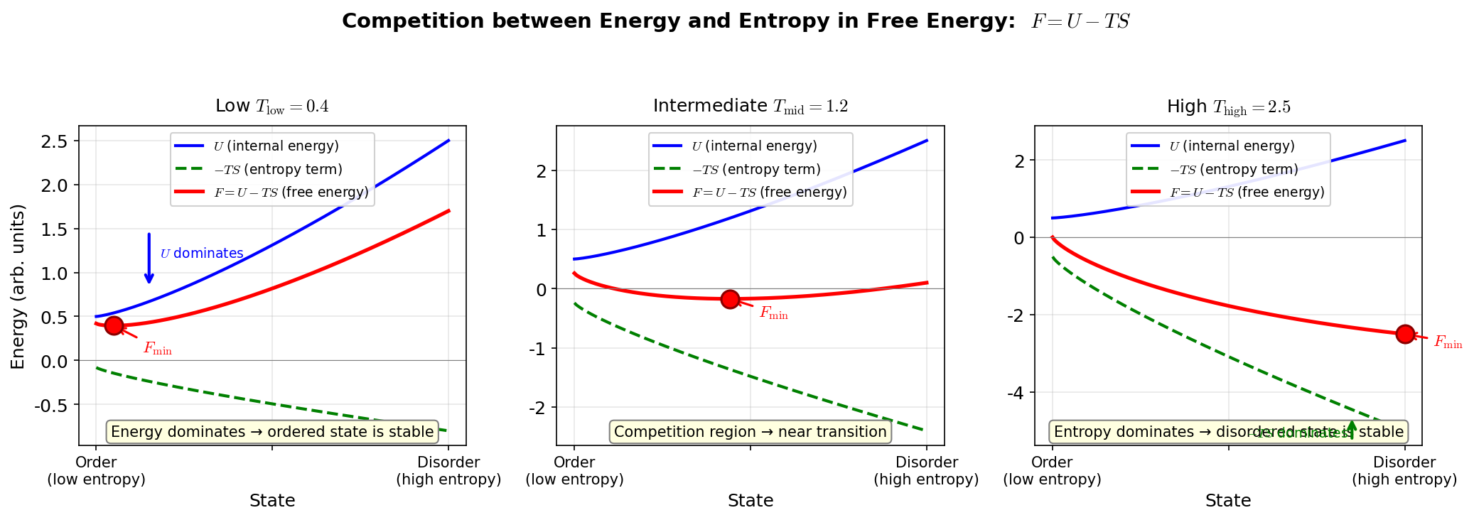
Fig. 3.9: Competition between energy and entropy in free energy. In \(F = U - TS\), energy minimization (order) dominates at low temperature, while entropy maximization (disorder) dominates at high temperature.
🟡 Lina: The essence of phase transitions is that the minimization condition for \(F\) changes with temperature.
Differential Form
🟡 Lina: Computing the infinitesimal change of \(F\):
Substituting \(dU = T\,dS - p\,dV\):
🔵 Kai: Oh, the \(T\,dS\) canceled cleanly!
🟡 Lina: The natural variables of \(F\) are \((T, V)\). From partial derivatives:
⚪ Mei: If you know a single function \(F\), differentiating with respect to \(T\) gives entropy and with respect to \(V\) gives pressure—everything comes out.
✅ Comprehension Check: Under what conditions is the free energy \(F = U - TS\) minimized?
Answer
At constant temperature and constant volume, the system changes in the direction that minimizes the free energy \(F\).
3.9 From "Necessity" to "Fundamental Laws of the Universe"
🟡 Lina: Let's step back and review the story of this chapter.
🔵 Kai: It started from the practical question of wanting to improve steam engine efficiency.
⚪ Mei: From there, Carnot's efficiency limit emerged, connecting to the Second Law and then to Boltzmann's \(S = k_B \ln \Omega\).
🔵 Kai: But isn't it strange? Carnot was only thinking about steam engine efficiency—why did he arrive at a law that applies to the entire universe?
🟡 Lina: Good question. Because Carnot pursued the "ideal limit." The moment he discarded the details of specific machines and asked "what is possible in principle?", the problem transcended any particular machine and became universal. An inquiry that began from the practical necessity of steam engines ultimately reached a fundamental property of the universe—entropy increases. In the prologue I said "motivations come in two types: necessity and curiosity," but even starting from necessity, you can reach depths just as profound as curiosity can.
✅ Comprehension Check: What practical question did this chapter's story begin with, and what fundamental property of the universe did it ultimately reach?
Answer
It began with the practical question of wanting to improve steam engine efficiency, and ultimately reached the fundamental property of the universe that "entropy increases."
3.10 Foreshadowing: Entropy and Black Holes
%%{init: {"theme": "default", "themeCSS": ".edgePath .path, .flowchart-link { stroke-width: 2px !important; }"}}%%
flowchart TD
    A["Steam engine efficiency<br/>(practical motivation)"] --> B["Carnot cycle<br/>η = 1 − T_C/T_H"]
    B --> C["Second Law of Thermodynamics<br/>Entropy increase"]
    C --> D["Boltzmann<br/>S = k_B ln Ω"]
    D --> E["Statistical mechanics<br/>Counting microstates"]
    E --> F["Bekenstein-Hawking<br/>Black hole entropy<br/>S_BH = A/(4ℓ_P²) k_B"]
    F --> G["Strominger-Vafa (1996)<br/>Computing microstates with string theory<br/>(Chapter 20)"]
    style A fill:#ffa,stroke:#333
    style G fill:#afa,stroke:#333
Fig. 3.10: Genealogy of the entropy concept
🟡 Lina: Let me plant one piece of foreshadowing.
🔵 Kai: Foreshadowing?
🟡 Lina: The concept of entropy we learned in this chapter will reappear in later chapters. In the 1970s, Bekenstein and Hawking showed that black holes also have entropy:
Here \(A\) is the area of the event horizon, \(\hbar = h/(2\pi)\) is the Dirac constant (Planck's constant \(h\) divided by \(2\pi\); in quantum mechanics this appears more frequently than \(h\)—you'll see why from the next chapter onward; for now think of it as "a constant related to \(h\)"), and \(\ell_P = \sqrt{G\hbar/c^3}\) is the Planck length (which we'll treat in more detail in later chapters).
🔵 Kai: Black holes have entropy... so from \(S = k_B \ln \Omega\), does that mean black holes also have microstates?
🟡 Lina: That very question leads to one of string theory's greatest successes. In 1996, Strominger and Vafa used string theory to count the microstates of black holes and derived the Bekenstein-Hawking entropy from \(S = k_B \ln \Omega\) (Ch. 20).
⚪ Mei: A concept that started with steam engines connects to black holes!
🟡 Lina: That's what makes physics fascinating. Fields that seem unrelated are connected at deep levels. But be careful—the Bekenstein-Hawking entropy comes from combining general relativity and quantum mechanics, and while its microscopic origin has been explained by string theory, this is limited to specific black holes (BPS black holes). Extension to general black holes remains an unsolved problem.
🔭 Philosophy of Science Note: The derivation of black hole entropy from string theory is a beautiful achievement, but by itself it doesn't constitute "experimental verification" of string theory. This is because other models (such as loop quantum gravity) might also be able to derive the same result. "A model that gives the right answer" and "the uniquely correct model" are different things. From the standpoint of falsifiability, judge for yourself.
✅ Comprehension Check: Who showed that black holes also have entropy?
Answer
Bekenstein and Hawking.
Preview of the Next Chapter
Ch. 4 — The three successful models of Newtonian mechanics, electromagnetism, and thermodynamics begin to fail one after another at the end of the 19th century. Black-body radiation, the photoelectric effect, the precession of Mercury's perihelion. This "crisis" opens the door to the two great revolutions of the 20th century—relativity and quantum mechanics. In particular, the black-body radiation problem plays an important role as the intersection of thermodynamics learned in this chapter and quantum theory (see Quantum Mechanics Ch. 1 of Quantum Mechanics for details).
References
The content of this chapter was structured with reference to the following sources.
- David Tong, Lectures on Statistical Physics, Ch.1: "The Fundamentals of Statistical Mechanics" — Microcanonical ensemble, principle of equal a priori probabilities
- David Tong, Lectures on Statistical Physics, Ch.2: "Classical Gases" — Boltzmann entropy, statistical mechanical definition of temperature
- David Tong, Lectures on Statistical Physics, Ch.4: "Classical Thermodynamics" — Laws of thermodynamics, Carnot cycle
- David Tong, Lectures on Statistical Physics, Ch.5: "Phase Transitions" — Free energy
Feedback on this page
Let us know if something was unclear, incorrect, or could be improved.