Appendix D: Curvature Quantities for Representative Spacetimes: Formula Collection
Story so far: Through Appendix C, we have established the computational techniques of tensor analysis and the tools of differential forms. Throughout the main text, we have dealt with many specific spacetimes, including the Schwarzschild spacetime, general spherically symmetric spacetimes, and the Friedmann-Robertson-Walker (FRW) cosmological model. However, searching through scattered results across chapters each time is cumbersome.
Goals of this chapter
- Organize the metric, Christoffel symbols, Riemann curvature tensor, and Einstein tensor for representative spacetimes appearing throughout all chapters as a reference table
- Complete a formula collection that can be repeatedly referenced as a "dictionary" for future applications and exercises
🟡 Lina: Well, you two. It's been a long journey. Starting from special relativity, through curved spacetime, geodesics, black holes, cosmology, and the Einstein equations—you've learned an enormous amount of material.
🔵 Kai: Honestly, my head is about to explode... The Schwarzschild Christoffel symbols, the FRW Einstein tensor—I keep going "wait, what was that again?"
⚪ Mei: Same here. Recalculating from scratch every time just isn't realistic.
🟡 Lina: That's exactly why we're creating this chapter. Think of it like bringing a formula sheet to an exam—I want you to use this as a general relativity dictionary. We won't just compile calculation "results"; we'll also confirm the physical meaning of each quantity as we go.
D.1 Review of Basic Definitions
🟡 Lina: First, let me gather all the geometric quantities appearing in this formula collection in one place. This also serves as a summary of what we learned from Chapter 4 onward in the main text. For an overview of the three main metrics covered in this chapter, see Fig. D.1 "Comparison of key metrics". Minkowski (flat), Schwarzschild (spherically symmetric vacuum), and FRW (homogeneous isotropic universe)—these three are the most fundamental metrics in general relativity.
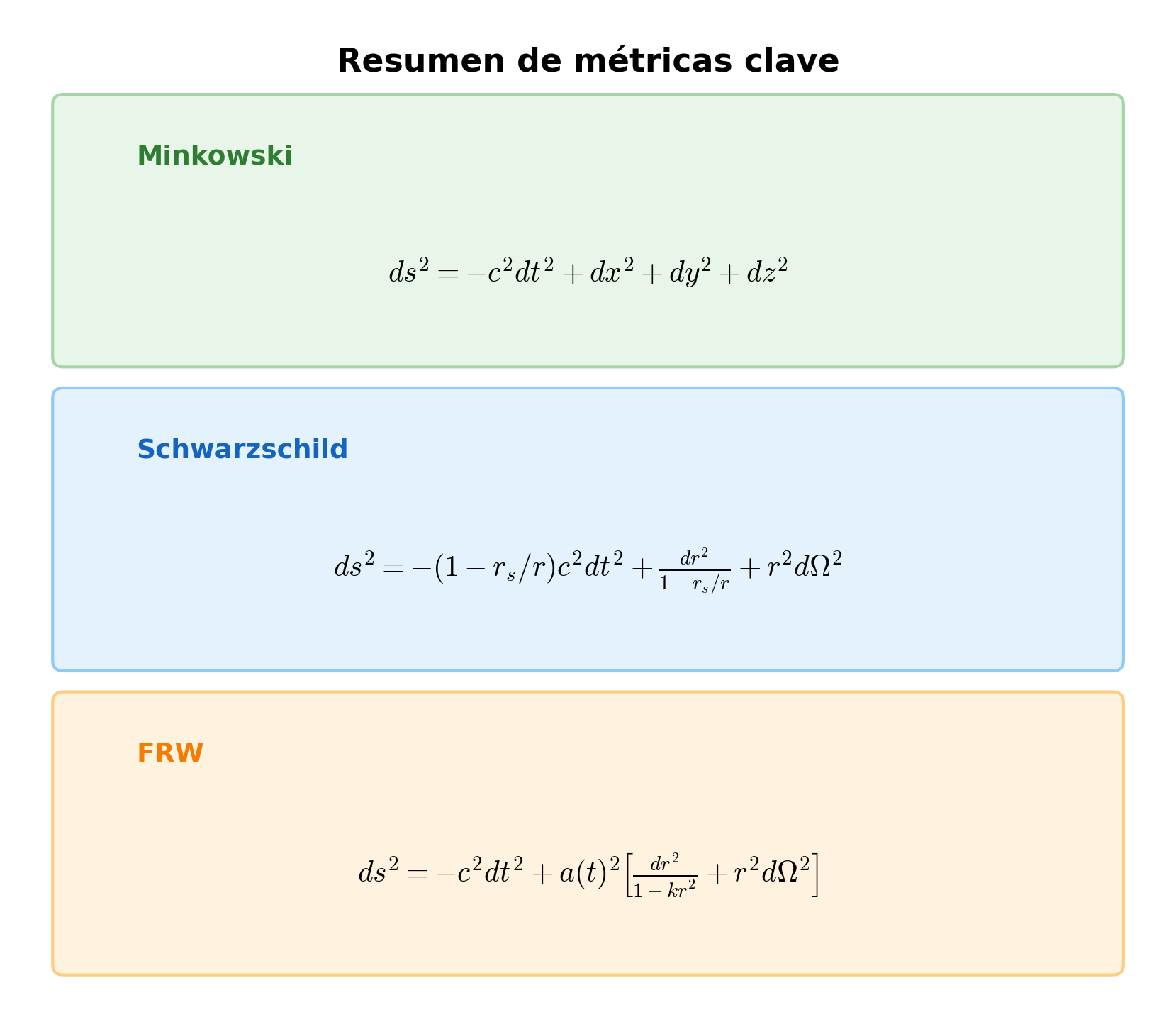
Fig. D.1: Comparison of key metrics. The three main metrics: Minkowski, Schwarzschild, and FRW.
D.1.1 Metric Tensor
🟡 Lina: The metric tensor \(g_{\alpha\beta}\) is the "ruler" of spacetime. It defines the line element between two points as
In flat Minkowski spacetime, \(g_{\alpha\beta} = \eta_{\alpha\beta} = \mathrm{diag}(-1, +1, +1, +1)\). In the presence of gravity, \(g_{\alpha\beta}\) becomes a function of the coordinates.
🔵 Kai: The metric tensor represents "the gravitational field itself," right?
🟡 Lina: Exactly. In Newton's model, the gravitational potential \(\Phi\) represented the gravitational field, but in Einstein's model, the metric tensor \(g_{\alpha\beta}\) takes on that role.
D.1.2 Christoffel Symbols
🟡 Lina: As you can see from the definition, swapping \(\nu\) and \(\sigma\) doesn't change the right-hand side. In other words, it's symmetric in the lower indices: \(\Gamma^\mu{}_{\nu\sigma} = \Gamma^\mu{}_{\sigma\nu}\). This reduces the number of independent components by nearly half.
⚪ Mei: So it's a property that follows automatically from the structure of the definition.
🟡 Lina: Physically, this is the quantity that appears in the geodesic equation
It tells us what it means to "travel straight" in curved spacetime.
D.1.3 Riemann Curvature Tensor
🔵 Kai: A rank-4 tensor... just looking at the formula, I can't get any intuition for what it represents. How is it related to tidal forces?
🟡 Lina: Intuitively, think of two particles falling freely side by side—the Riemann tensor determines their "relative acceleration," whether they move toward or away from each other. If you drop two balls one above the other near Earth, the lower ball experiences stronger gravity so their separation increases, right? That's the tidal force, and the Riemann tensor precisely describes its magnitude and direction.
Now, as a rank-4 tensor, each index takes values 0–3, giving \(4^4 = 256\) total components. But due to symmetries, only 20 are independent. Let me outline how to count them:
- \(R_{\alpha\beta\gamma\delta} = -R_{\beta\alpha\gamma\delta}\) (antisymmetry in the 1st and 2nd indices)
- \(R_{\alpha\beta\gamma\delta} = -R_{\alpha\beta\delta\gamma}\) (antisymmetry in the 3rd and 4th indices)
- \(R_{\alpha\beta\gamma\delta} = R_{\gamma\delta\alpha\beta}\) (exchange symmetry of the first and second pairs)
- \(R_{\alpha\beta\gamma\delta} + R_{\alpha\gamma\delta\beta} + R_{\alpha\delta\beta\gamma} = 0\) (first Bianchi identity: the cyclic sum over the 2nd–4th indices vanishes)
From the first two antisymmetries, the pair \([\alpha\beta]\) has \(\binom{4}{2} = 6\) choices, and the pair \([\gamma\delta]\) also has 6 choices. So there are \(6 \times 6 = 36\) independent combinations. Furthermore, due to the third symmetry (exchange of the first and second pairs), swapping \([\alpha\beta]\) and \([\gamma\delta]\) gives the same value. Here, let me use a convenient technique for counting independent components. A rank-4 tensor with 4 indices is complicated, but thanks to the antisymmetries, we can treat each pair \([\alpha\beta]\) and \([\gamma\delta]\) as "a single label." Since there are 6 choices for each pair, we can rearrange the independent components of \(R_{\alpha\beta\gamma\delta}\) into a \(6 \times 6\) table (matrix). Consider a \(6 \times 6\) matrix with the 6 choices of \([\alpha\beta]\) as row numbers and the 6 choices of \([\gamma\delta]\) as column numbers. Specifically, label the 6 antisymmetric pairs as \([01], [02], [03], [12], [13], [23]\) with numbers \(i = 1, 2, \ldots, 6\), and construct the matrix \(M_{ij} = R_{[\alpha\beta]_i [\gamma\delta]_j}\). For example, \(M_{12} = R_{0102}\) (the combination of pair \([01]\) and pair \([02]\)), \(M_{21} = R_{0201}\) (the combination of pair \([02]\) and pair \([01]\)), and the exchange symmetry \(R_{\alpha\beta\gamma\delta} = R_{\gamma\delta\alpha\beta}\) gives \(M_{12} = M_{21}\). In general, this exchange symmetry corresponds to the matrix symmetry \(M_{ij} = M_{ji}\).
🔵 Kai: I see, so you "compress" the rank-4 tensor into a rank-2 matrix to get a clearer picture. I know how to count independent components of a symmetric matrix.
🟡 Lina: Exactly. In a symmetric matrix, the \((i,j)\) and \((j,i)\) components are equal, so the independent components are just the "diagonal elements" and the "elements above the diagonal." For a \(6 \times 6\) matrix, there are 6 diagonal elements and \(5 + 4 + 3 + 2 + 1 = 15\) off-diagonal elements above the diagonal (the 1st row has 5 to its right, the 2nd row has 4, and so on). Together that's \(6 + 15 = 21\). This is the general formula \(n(n+1)/2\) for an \(n \times n\) symmetric matrix with \(n = 6\).
⚪ Mei: So we're at 21 so far. But there was one more symmetry in the list earlier, wasn't there?
🟡 Lina: Good memory. That's right, the Bianchi identity hasn't been used yet. \(R_{\alpha\beta\gamma\delta} + R_{\alpha\gamma\delta\beta} + R_{\alpha\delta\beta\gamma} = 0\)—this provides a new constraint only when all four indices are distinct. When there are repeated indices, each term becomes zero or cancels with others due to antisymmetry, making the identity trivially satisfied.
🔵 Kai: Specifically, what does that mean?
🟡 Lina: Let me show you just one of the clearest examples. If \(\alpha = \beta\), the first term is \(R_{\alpha\alpha\gamma\delta} = 0\) (when the same index appears in the first two positions, antisymmetry forces it to zero). The remaining terms similarly vanish, giving \(0 + 0 + 0 = 0\), which is trivial. Other patterns of repetition (for example \(\gamma = \alpha\)) can similarly be verified to be trivially satisfied—try it as a practice exercise if you're interested.
⚪ Mei: So the only case that gives genuinely new information is when all four indices are distinct.
🟡 Lina: Exactly. In 4 dimensions, consider using all four values \((0,1,2,3)\). The Bianchi identity is a cyclic sum over the 2nd–4th indices with the 1st index \(\alpha\) fixed. There are 4 choices for \(\alpha\), but actually they all reduce to the same equation. Let's look at this concretely. Choosing \(\alpha = 0\) gives \(R_{0123} + R_{0231} + R_{0312} = 0\). Next, choosing \(\alpha = 1\) gives \(R_{1023} + R_{1230} + R_{1302} = 0\). However, using the symmetries, this equation reduces to the same content as the \(\alpha = 0\) case.
🔵 Kai: Wait, different \(\alpha\) gives the same equation?
🟡 Lina: Yes. For example, \(R_{1023}\) directly gives \(R_{1023} = -R_{0123}\) from the antisymmetry of the first two indices \(R_{\alpha\beta\gamma\delta} = -R_{\beta\alpha\gamma\delta}\) (just swapping indices 1 and 0). Similarly for \(R_{1230}\), using the pair exchange symmetry \(R_{\alpha\beta\gamma\delta} = R_{\gamma\delta\alpha\beta}\) gives \(R_{1230} = R_{3012}\), and then the first-pair antisymmetry gives \(R_{3012} = -R_{0312}\), which reduces to the third term of the \(\alpha = 0\) equation. \(R_{1302}\) also reduces to the second term of the \(\alpha = 0\) equation by the same procedure (the remaining cases \(\alpha = 2, 3\) can be verified similarly—try them as practice exercises). So there is only 1 independent Bianchi identity. Ultimately, \(21 - 1 = 20\) independent components remain.
⚪ Mei: You narrow it down step by step using each symmetry: 256 → 36 → 21 → 20. What a beautiful structure.
D.1.4 Ricci Tensor and Scalar Curvature
🟡 Lina: Since the Riemann tensor is rank-4 and contains too much information, we "contract" one pair of indices (that is, set one upper index and one lower index to the same letter and sum over them) to obtain a rank-2 tensor—the Ricci tensor \(R_{\mu\nu}\). Looking at the definition \(R_{\mu\nu} = R^\rho{}_{\mu\rho\nu}\), the 1st index (upper \(\alpha\)) and the 3rd index (lower \(\gamma\)) of the original Riemann tensor \(R^\alpha{}_{\beta\gamma\delta}\) are set to the same letter \(\rho\) and summed over \(\rho = 0, 1, 2, 3\). The remaining 2nd and 4th indices become \(\mu\) and \(\nu\) of the Ricci tensor. While the Riemann tensor records the "tidal force in each direction," the Ricci tensor summarizes this into "volume change along a given direction." Specifically, it represents the rate at which a small freely falling sphere is compressed or stretched by the gravity of surrounding matter, changing its volume.
🔵 Kai: How does "summing up tidal forces in each direction" become "volume change"?
🟡 Lina: Good question. Think of a small sphere. The Riemann tensor records deformations individually: "compressed in the \(x\) direction," "stretched in the \(y\) direction," "compressed in the \(z\) direction," and so on. The contraction in the Ricci tensor \(R_{\mu\nu}\) corresponds to summing these deformations over all directions. If you total the deformations in all directions, you can tell whether the overall volume of the sphere increases or decreases, right? That's why contraction corresponds to volume change. Furthermore, its trace (the average over all directions) is the scalar curvature \(R\). The Einstein tensor is constructed from these two.
⚪ Mei: Riemann is "tidal force in each direction," and Ricci is its "summary"—the result of summing deformations over all directions.
🟡 Lina: Exactly.
D.1.5 Einstein Tensor
🟡 Lina: The Einstein equation is (in geometric units \(G = c = 1\))
The left side \(G_{\mu\nu}\) is the curvature of spacetime, and the right side \(T_{\mu\nu}\) is the distribution of energy and momentum. The reason \(G_{\mu\nu}\) rather than \(R_{\mu\nu}\) appears on the left side is that \(G_{\mu\nu}\) automatically satisfies the identity \(\nabla^\mu G_{\mu\nu} = 0\) (derived from the Bianchi identity). Here \(\nabla_\mu\) is the covariant derivative—the differential operator in curved spacetime that adds correction terms involving Christoffel symbols to the ordinary partial derivative \(\partial_\mu\) (we studied this in detail in Ch. 12 of the main text). Intuitively, think of it as "a derivative that extracts the true rate of change of a tensor without being misled by the bending of the coordinate system." \(\nabla^\mu\) is shorthand for \(g^{\mu\alpha}\nabla_\alpha\), meaning the covariant derivative with its index raised by the metric. To be specific about what \(\nabla^\mu G_{\mu\nu} = 0\) means: since \(\mu\) in \(\nabla^\mu\) and the first \(\mu\) in \(G_{\mu\nu}\) are the same letter appearing as upper and lower indices, by Einstein's summation convention we sum over \(\mu = 0, 1, 2, 3\). That is, \(\nabla^0 G_{0\nu} + \nabla^1 G_{1\nu} + \nabla^2 G_{2\nu} + \nabla^3 G_{3\nu} = 0\) holds for each \(\nu\)—this is what "the covariant divergence vanishes" means.
🔵 Kai: So it's like the ordinary "divergence" but with corrections for curved spacetime.
🟡 Lina: Exactly. If you do the same thing with ordinary partial derivatives \(\partial^\mu\), you get the "ordinary divergence," but \(\nabla^\mu\) includes corrections from Christoffel symbols, making it the "correct divergence even in curved spacetime." The structure is just the sum shown above, but the contents of each term are slightly more complex than with partial derivatives—that's the only difference. This identity is consistent with the energy conservation law \(\nabla^\mu T_{\mu\nu} = 0\) on the right side, making the equation self-consistent. In other words, the matter distribution on the right determines the curvature on the left, and conversely, that curvature determines the motion of matter through geodesics. In Wheeler's famous words: "Matter tells spacetime how to curve, and spacetime tells matter how to move."
⚪ Mei: The energy conservation law and the geometric identity are automatically consistent—that's why the Einstein tensor is the appropriate quantity for the left side of the equation.
D.1.6 Orthonormal Basis (Tetrad)
🟡 Lina: Let me first explain why we introduce an "orthonormal basis" here. Components of the Riemann tensor or Einstein tensor written in a coordinate basis depend on the choice of coordinates and acquire complicated factors. But when written in an orthonormal basis, each component directly corresponds to a local physical quantity (magnitude of tidal forces, energy density, pressure, etc.). That's why many entries in this formula collection give curvature quantities in orthonormal basis components.
🟡 Lina: Recall that the metric tensor \(g_{\alpha\beta}\) is the tool for computing the inner product of two vectors. It generalizes the high school vector dot product \(\mathbf{u} \cdot \mathbf{v} = u_x v_x + u_y v_y + u_z v_z\). In curved spacetime it's written as \(g(\mathbf{u}, \mathbf{v}) = g_{\alpha\beta}u^\alpha v^\beta\) (the same indices \(\alpha\), \(\beta\) appear as upper and lower, so we sum each over 0–3—Einstein's summation convention). In flat space, \(g_{\alpha\beta}\) becomes the identity matrix and you recover the high school dot product formula. Now I'll introduce "hatted indices" \(\hat{\alpha}\). These denote orthonormal basis indices, distinguishing them from coordinate basis indices \(\alpha\). When a basis \(\mathbf{e}_{\hat{\alpha}}\) labeled with hatted indices \(\hat{\alpha}\) satisfies
—that is, when the inner products of the basis vectors equal the Minkowski metric \(\eta_{\hat{\alpha}\hat{\beta}} = \mathrm{diag}(-1,+1,+1,+1)\)—we call it an "orthonormal basis." It corresponds to the basis of a "freely falling elevator" where special relativity holds locally. For a diagonal metric \(ds^2 = g_{00}(dx^0)^2 + g_{11}(dx^1)^2 + \cdots\), each basis vector is obtained simply by taking the reciprocal of the square root of the absolute value of the metric component. The notation \((\mathbf{e}_{\hat{\alpha}})^\mu\) means "the \(\mu\)-direction coordinate component of basis vector \(\mathbf{e}_{\hat{\alpha}}\)." For a diagonal metric, the \(\hat{\alpha}\)-th orthonormal basis vector has a component only in the same coordinate direction as \(\hat{\alpha}\). Let me show a specific example first. For \(\hat{\alpha} = \hat{r}\), the basis vector \(\mathbf{e}_{\hat{r}}\) has a component only in the \(r\) direction, with value \(1/\sqrt{|g_{rr}|}\). Its components in the other directions (\(t\), \(\theta\), \(\varphi\)) are all zero. Writing this generally: \((\mathbf{e}_{\hat{\alpha}})^\mu = \delta^\mu_\alpha / \sqrt{|g_{\alpha\alpha}|}\). Here \(\delta^\mu_\alpha\) is called the Kronecker delta, which equals 1 when \(\mu = \alpha\) and 0 when \(\mu \neq \alpha\). In other words, it expresses mathematically that "there is a component only in the \(\alpha\) direction." One point to note: the \(\alpha\) in this formula is a fixed label indicating "the coordinate direction corresponding to \(\hat{\alpha}\)," and is not an index to be summed over by Einstein's summation convention. Normally when the same letter appears as upper and lower indices we sum, but here we're just specifying one direction for each \(\hat{\alpha}\), like "the direction corresponding to \(\hat{r}\) is \(r\)." Let me give you a tip for recognizing this: \(\delta^\mu_\alpha\) is a table of values meaning "1 if \(\mu = \alpha\), 0 if \(\mu \neq \alpha\)," not an instruction to sum over \(\alpha\). Here \(\alpha\) is a fixed label specifying "which orthonormal basis vector we're talking about"—for example, when writing the \(\hat{r}\) basis, we fix \(\alpha = r\), and only \(\mu\) runs over \(t, r, \theta, \varphi\). As a result, only the \(\mu = r\) component is \(1/\sqrt{|g_{rr}|}\), and the rest are zero. In practice, you don't need to memorize the general formula—just remember that "the basis vector in the \(\hat{\alpha}\) direction has a component of \(1/\sqrt{|g_{\alpha\alpha}|}\) in the corresponding coordinate direction." Written out explicitly: for \(\hat{t}\), it's \(1/\sqrt{|g_{tt}|}\) in the \(t\) direction; for \(\hat{r}\), it's \(1/\sqrt{g_{rr}}\) in the \(r\) direction; for \(\hat{\theta}\), it's \(1/\sqrt{g_{\theta\theta}}\) in the \(\theta\) direction; for \(\hat{\varphi}\), it's \(1/\sqrt{g_{\varphi\varphi}}\) in the \(\varphi\) direction—that's all there is to it.
When converting tensor components to the orthonormal basis, you use the basis vector components: \(T_{\hat{\alpha}\hat{\beta}} = (\mathbf{e}_{\hat{\alpha}})^\mu (\mathbf{e}_{\hat{\beta}})^\nu T_{\mu\nu}\). For a diagonal metric, this simply reduces to "dividing by \(\sqrt{|g_{\alpha\alpha}|}\) for each index"—because the basis vector components are \(1/\sqrt{|g_{\alpha\alpha}|}\). We'll use this conversion rule concretely in D.3.3.
🔵 Kai: This is a bit hard to visualize. Multiplying by the basis vector components basically means "normalizing the scale markings of the coordinate basis," right?
🟡 Lina: Yes, that's a good way to put it. Coordinate basis vectors have "tick mark lengths" that vary from place to place, right? The orthonormal basis adjusts them all to unit length, so when converting tensor components, you divide by the "tick mark size"—that's what multiplying by \(1/\sqrt{|g_{\alpha\alpha}|}\) corresponds to. Let's see what this looks like concretely.
🟡 Lina: For example, in Schwarzschild spacetime where \(g_{rr} = (1-2M/r)^{-1}\), we have \(|g_{rr}|^{1/2} = (1-2M/r)^{-1/2}\), and its reciprocal \((1-2M/r)^{1/2}\) becomes the \(r\) component of the \(\hat{r}\) basis vector. All components are listed in D.2.3, so you can check there.
⚪ Mei: So in any curved spacetime, you can always find a basis that locally looks like the Minkowski metric \(\eta_{\hat{\alpha}\hat{\beta}}\) of special relativity.
✅ Comprehension Check: Why does the Riemann curvature tensor in 4-dimensional spacetime have only 20 independent components?
Answer
The Riemann tensor has multiple symmetries: antisymmetry in the 1st and 2nd indices, antisymmetry in the 3rd and 4th indices, exchange symmetry of the first and second pairs, and the first Bianchi identity (the cyclic sum over the 2nd–4th indices vanishes). These constraints reduce the original \(256\) components to only 20 independent ones.
D.2 Schwarzschild Spacetime
🟡 Lina: The vacuum spacetime around a non-rotating, spherically symmetric mass \(M\). Planetary motion in the solar system, light bending, the most basic black hole model—everything derives from here. Take a look at Fig. D.2 "Mass-radius relation of astronomical objects and the Schwarzschild radius". It compares the mass and radius of various astronomical objects on a log-log plot, from Earth to the galactic center black hole (Sgr A*). The black line is the Schwarzschild radius, which in geometric units (\(G = c = 1\), see D.6 for details) is \(r_s = 2M\), and in SI is \(r_s = 2GM/c^2\). When an object's radius becomes smaller than this, it becomes a black hole. Looking at the figure, neutron stars sit just above the black line with only a factor of a few to spare from the Schwarzschild radius—meaning their compactness \(GM/(Rc^2)\) (a dimensionless quantity measuring how close the object's radius \(R\) is to the Schwarzschild radius \(2GM/c^2\), see Ch. 18 in the main text) is very high, as you can see at a glance.
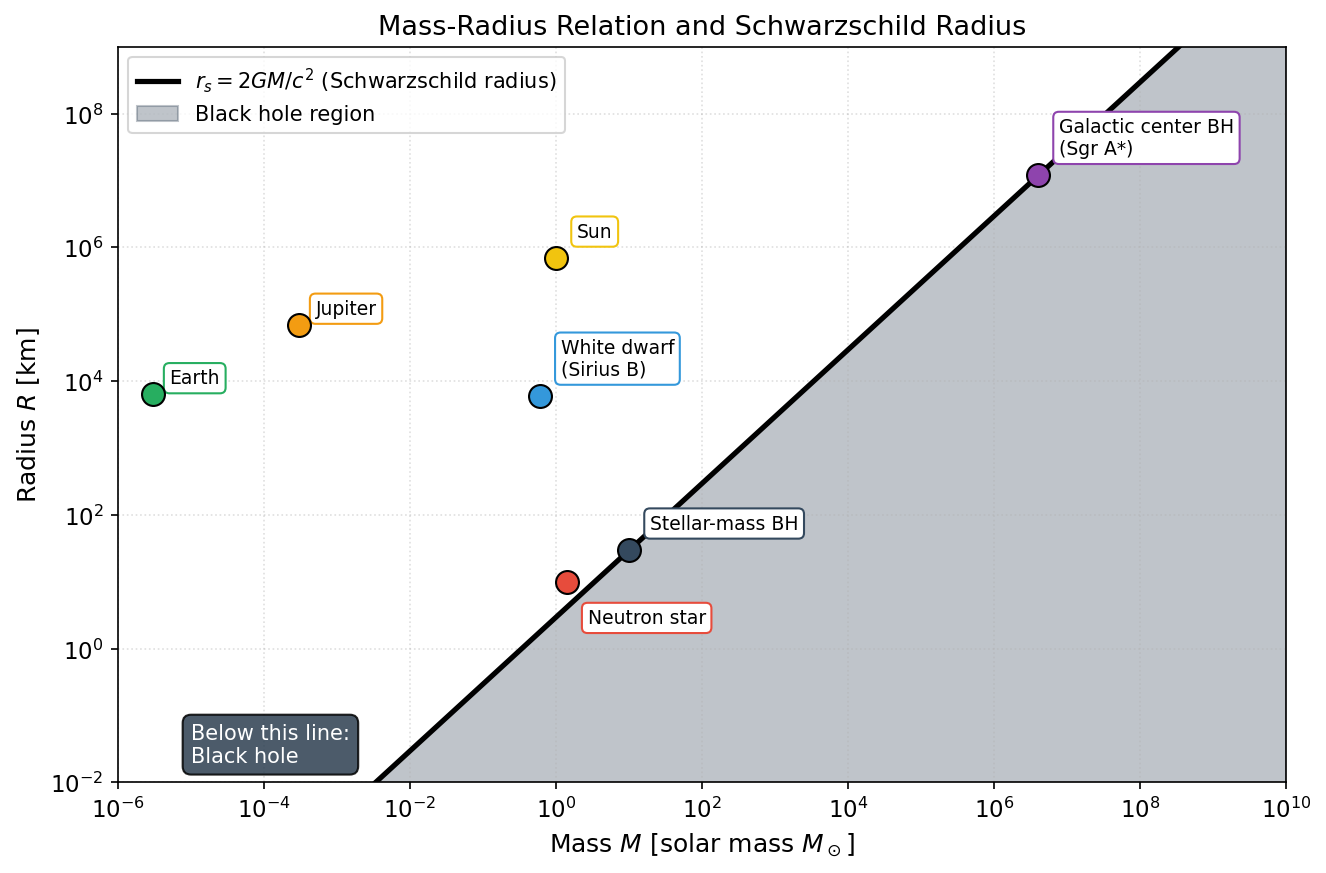
Fig. D.2: Mass-radius relation of astronomical objects and the Schwarzschild radius. Mass-radius relation and the Schwarzschild radius \(r_s = 2GM/c^2\) (in geometric units, \(r_s = 2M\)). Earth, Jupiter, the Sun, white dwarfs, neutron stars, stellar-mass black holes, and the galactic center black hole (Sgr A) compared on a log-log plot. The region below the black line (\(R < r_s\)) is a black hole.*
D.2.1 Metric
🔵 Kai: At \(r = 2M\), \(g_{tt} = 0\) and \(g_{rr}\) diverges, right? Is there really a "wall" there?
🟡 Lina: Good question. \(r = 2M\) is the event horizon, but it's merely a coordinate singularity. The Riemann tensor is finite there, so physically nothing special happens. The real singularity is at \(r = 0\).
✅ Comprehension Check: In Schwarzschild spacetime, what is the difference between the singularities at \(r = 2M\) and \(r = 0\)?
Answer
\(r = 2M\) is a coordinate singularity that can be removed by an appropriate coordinate transformation. In fact, the Riemann tensor takes finite values there. On the other hand, \(r = 0\) is a genuine (physical) singularity where curvature invariants (such as the Kretschner scalar \(R_{\alpha\beta\gamma\delta}R^{\alpha\beta\gamma\delta}\)) diverge.
D.2.2 Christoffel Symbols (Non-zero Components)
⚪ Mei: Using the lower-index symmetry, we also get \(\Gamma^t{}_{rt} = \Gamma^t{}_{tr}\), \(\Gamma^\theta{}_{\theta r} = \Gamma^\theta{}_{r\theta}\), and so on.
🟡 Lina: Look at \(\Gamma^r{}_{tt}\). Far away where \(r \gg 2M\), we have \((1 - 2M/r) \approx 1\), so \(\Gamma^r{}_{tt} \approx M/r^2\). This is exactly the Newtonian gravitational acceleration \(GM/r^2\) (with \(G = 1\)). Substituting into the geodesic equation reproduces Newton's equation of motion.
📝 Exercises:
- Derivation of \(\Gamma^r{}_{tt}\) → Problem B-1. Schwarzschild \(\Gamma^r_{\ tt}\), derivation of \(\Gamma^r{}_{rr}\) → Problem B-2. Schwarzschild \(\Gamma^r_{\ rr}\), verification of orthonormal basis → Problem B-6. Verification of the Schwarzschild Orthonormal Basis, correspondence with general spherically symmetric metric → Problem B-7. Christoffel Symbol Verification for General Spherical Symmetry
D.2.3 Orthonormal Basis
🔵 Kai: Since \(g_{tt} = -(1-2M/r)\), we have \(|g_{tt}|^{1/2} = (1-2M/r)^{1/2}\). Its reciprocal becomes the \(t\) component of the \(\hat{t}\) basis vector... But wait, at \(r = 2M\), \((1-2M/r)^{-1/2}\) diverges, right? Does that mean we can't construct an orthonormal basis?
🟡 Lina: Sharp observation. The orthonormal basis based on the coordinate \(t\) indeed breaks down at \(r = 2M\). This reflects the coordinate singularity, and to cross the horizon one needs to switch to a different coordinate system (for example, one using the proper time of a freely falling observer).
D.2.4 Riemann Curvature (Orthonormal Basis Components)
🟡 Lina: These are all the independent non-zero components—6 in total (in a general 4-dimensional spacetime there can be up to 20, but spherical symmetry imposes strong constraints). Moreover, thanks to spherical symmetry, the \(\theta\) and \(\varphi\) directions are equivalent, which is why some of the equations above have pairs connected by equality signs. In terms of independent "values," there are really only 4 types (\(\pm 2M/r^3\) and \(\pm M/r^3\)). The remaining non-zero components are determined by symmetries. For example, \(R_{\hat{t}\hat{r}\hat{r}\hat{t}}\) follows from the antisymmetry of the 1st and 2nd indices: \(R_{\hat{t}\hat{r}\hat{r}\hat{t}} = -R_{\hat{r}\hat{t}\hat{r}\hat{t}} = 2M/r^3\). Also, components mixing different angular directions (such as \(R_{\hat{t}\hat{\theta}\hat{r}\hat{\varphi}}\)) vanish due to spherical symmetry. Intuitively, in a spherically symmetric spacetime the \(\theta\) and \(\varphi\) directions are "equivalent," so there's no reason for one to couple specially with others—hence the mixed components must vanish. Everything has \(M/r^3\) as the basic scale, with coefficients being just \(\pm 1\) or \(\pm 2\). The same \(r^{-3}\) dependence as the Newtonian tidal force.
🔵 Kai: They're all proportional to \(r^{-3}\). So how large are they at \(r = 2M\) (the horizon)?
🟡 Lina: For example, substituting \(r = 2M\) into \(R_{\hat{\theta}\hat{t}\hat{\theta}\hat{t}} = M/r^3\) gives \(1/(8M^2)\), which is finite. The more massive the black hole, the larger \(M\) is, so the tidal force at the horizon is actually weaker. But at \(r = 0\) it diverges—that's the real singularity.
⚪ Mei: Since it's \(1/(8M^2)\), if \(M\) increases by a factor of 10, the tidal force decreases by a factor of 100. That clearly explains why the horizon of a supermassive black hole is "gentle."
🔵 Kai: At large distances \(r \to \infty\), all components approach zero. So far away it returns to flat spacetime?
🟡 Lina: Exactly. This is called asymptotic flatness. It's a property expected for the spacetime around an isolated body. By the way, while the Riemann tensor is non-zero, the Ricci tensor vanishes completely. Since it's a vacuum, \(R_{\mu\nu} = 0\).
🔵 Kai: Are \(R_{\mu\nu} = 0\) and \(G_{\mu\nu} = 0\) from D.2.5 the same thing?
🟡 Lina: Yes, in 4 dimensions they're equivalent. Contracting (taking the trace of) both sides of \(G_{\mu\nu} = R_{\mu\nu} - \frac{1}{2}g_{\mu\nu}R\) with \(g^{\mu\nu}\): \(g^{\mu\nu}R_{\mu\nu} = R\) (this is just the definition of \(R\)), and \(g^{\mu\nu}g_{\mu\nu} = \delta^\mu{}_\mu = 4\) (\(\delta^\mu{}_\mu\) adds up four 1's for \(\mu = 0,1,2,3\)), giving \(g^{\mu\nu}G_{\mu\nu} = R - \frac{1}{2} \cdot 4 \cdot R = R - 2R = -R\). So if \(G_{\mu\nu} = 0\), the trace gives \(R = 0\). Substituting back into \(G_{\mu\nu} = R_{\mu\nu} - \frac{1}{2}g_{\mu\nu}R = 0\) gives \(R_{\mu\nu} = 0\) as well. Conversely, if \(R_{\mu\nu} = 0\) then \(R = g^{\mu\nu}R_{\mu\nu} = 0\), so \(G_{\mu\nu} = R_{\mu\nu} = 0\). Try verifying this explicitly as a practice exercise.
⚪ Mei: Taking the trace gives the relation between \(R\) and \(G\), and substituting back proves the equivalence. An elegant argument.
🔵 Kai: Hmm... so in vacuum, \(R_{\mu\nu} = 0\) and \(G_{\mu\nu} = 0\) are the same—I get that. But the Riemann tensor is non-zero, right? So "zero curvature" and "zero Ricci" are completely different things. Then conversely, when matter is present, are \(R_{\mu\nu} = 0\) and \(G_{\mu\nu} = 0\) no longer equivalent?
🟡 Lina: Good question. When matter is present, \(G_{\mu\nu} = 8\pi T_{\mu\nu} \neq 0\), so neither is zero to begin with. But the mathematical fact that "\(R_{\mu\nu} = 0\) is equivalent to \(G_{\mu\nu} = 0\)" holds regardless of whether the right side is zero. And as we just confirmed, even in vacuum (\(R_{\mu\nu} = 0\)) the Riemann tensor is non-zero—meaning "spacetime can be curved even without matter." That's one of the fascinating aspects of general relativity.
✅ Comprehension Check: From what can the Christoffel symbols and Riemann tensor of Schwarzschild spacetime be mechanically computed?
Answer
They can be mechanically computed from the metric tensor \(g_{\mu\nu}\) and its partial derivatives. The Christoffel symbols are constructed from first derivatives of the metric, and the Riemann tensor from first derivatives of the Christoffel symbols and their quadratic products.
📝 Exercises:
- Symmetry of the Riemann tensor → Problem B-8. Application of Riemann Tensor Symmetries, verification that \(R_{\hat{t}\hat{t}} = 0\) → Problem B-9. Schwarzschild \(R_{tt} = 0\), computation of the Kretschmann scalar → Problem M-3. Kretschmann Scalar for Schwarzschild, geodesic equation and Newtonian limit → Problem M-1. Newtonian Limit of Schwarzschild Geodesics, circular orbits and tidal forces → Problem A-1. Schwarzschild Circular Orbits and Tidal Forces
D.2.5 Einstein Equation
🟡 Lina: A vacuum solution. The solution of the equation in regions without matter. The mass \(M\) enters the metric as a boundary condition.
D.3 General Spherically Symmetric Spacetime
🟡 Lina: A more general spherically symmetric spacetime that also allows time dependence. It describes gravitational collapse of stars and black hole formation processes.
D.3.1 Metric
🔵 Kai: Why write it with exponential functions like \(e^{\nu}\)? Couldn't we just use \(f(r,t)\)?
🟡 Lina: Good question. As we confirmed in D.1.1, our sign convention is \((-,+,+,+)\)—meaning the time direction gets a minus sign and spatial directions get plus signs in the \(ds^2\) expression. So \(g_{tt}\) must be negative and \(g_{rr}\) must be positive. Writing \(g_{tt} = -e^{\nu}\) and \(g_{rr} = e^{\lambda}\) guarantees \(e^{\nu} > 0\) and \(e^{\lambda} > 0\) regardless of what real values \(\nu\) and \(\lambda\) take, automatically maintaining the correct signs. Furthermore, the Christoffel symbols involve derivatives of the metric, right? Differentiating \(g_{rr} = e^{\lambda}\) gives \(\partial_r g_{rr} = \lambda' e^{\lambda}\), and when multiplied by \(g^{rr} = e^{-\lambda}\), the \(e^{\lambda}\) cancels, leaving just \(\lambda'\). So the Christoffel symbol expressions become much cleaner. Incidentally, the Schwarzschild solution is the special case \(e^{\nu} = e^{-\lambda} = 1 - 2M/r\) (time-independent). That is, \(\nu = -\lambda\) and both are functions of \(r\) only.
⚪ Mei: In the general case \(\nu\) and \(\lambda\) are independent functions, but in Schwarzschild that constraint is imposed.
D.3.2 Christoffel Symbols (Non-zero Components)
A dot \(\dot{}\) denotes \(\partial/\partial t\), and a prime \('\) denotes \(\partial/\partial r\).
🔵 Kai: Can we compare this with the Schwarzschild case? If I set \(\dot{\nu} = \dot{\lambda} = 0\) and substitute \(e^{\nu} = 1 - 2M/r\) and so on, would it match D.2.2?
🟡 Lina: Exactly. Let's actually substitute one and check. For example, substituting Schwarzschild values into \(\Gamma^r{}_{tt} = (\nu'/2)\,e^{\nu - \lambda}\): since \(e^\nu = 1-2M/r\), we have \(\nu = \ln(1-2M/r)\), and differentiating with respect to \(r\) gives \(\nu' = \frac{2M/r^2}{1-2M/r}\). Also \(e^{\nu-\lambda} = e^\nu \cdot e^{-\lambda} = (1-2M/r)(1-2M/r) = (1-2M/r)^2\). Substituting these: \(\frac{\nu'}{2}e^{\nu-\lambda} = \frac{M/r^2}{1-2M/r} \cdot (1-2M/r)^2 = \frac{M}{r^2}(1-2M/r)\). This matches D.2.2. You can also verify later that substituting the Schwarzschild values into the D.3.3 Einstein tensor formulas gives \(G_{\hat{t}\hat{t}} = 0\)—try that as a practice exercise.
D.3.3 Einstein Tensor (Orthonormal Basis Components)
The following are the diagonal components for the time-independent case (\(\dot{\nu} = \dot{\lambda} = 0\)). In the general time-dependent case, additional terms involving \(\dot{\lambda}\) and \(\dot{\nu}\) appear, but here we focus on the components most important for the static stellar interior structure.
🔵 Kai: Can we also verify that these become \(0\) for Schwarzschild?
🟡 Lina: Let's try. Substituting \(e^{-\lambda} = 1-2M/r\), \(e^\lambda = (1-2M/r)^{-1}\), and \(\nu' = \frac{2M/r^2}{1-2M/r}\): \(\nu' r = \frac{2M/r}{1-2M/r}\). Let's find a common denominator for the terms in the parentheses of \(G_{\hat{r}\hat{r}}\). Putting the 3 terms over the common denominator \((1-2M/r)\):
Expanding the numerator: \(2M/r + 1 - 2M/r - 1 = 0\). So the entire bracket vanishes and \(G_{\hat{r}\hat{r}} = 0\). Consistent with a vacuum solution.
⚪ Mei: It cancels out beautifully. I'd like to check \(G_{\hat{t}\hat{t}}\) too.
🟡 Lina: Let's verify \(G_{\hat{t}\hat{t}}\) similarly. For Schwarzschild, \(\nu = -\lambda\), so differentiating both sides with respect to \(r\) gives \(\nu' = -\lambda'\), meaning \(\lambda' = -\nu' = -\frac{2M/r^2}{1-2M/r}\). Substituting \(r\lambda' = -\frac{2M/r}{1-2M/r}\) into the bracket of \(G_{\hat{t}\hat{t}}\): \(-\frac{2M/r}{1-2M/r} - 1 + \frac{1}{1-2M/r} = \frac{-2M/r - (1-2M/r) + 1}{1-2M/r} = \frac{-2M/r - 1 + 2M/r + 1}{1-2M/r} = 0\), confirming \(G_{\hat{t}\hat{t}} = 0\) as well.
🔵 Kai: Oh, this one also cancels out to zero perfectly!
🟡 Lina: Let me also include one off-diagonal component that becomes non-zero when time dependence is present. Computing the Ricci tensor from the D.3.2 Christoffel symbols and constructing the Einstein tensor, the result in the coordinate basis is \(G_{tr} = \dot{\lambda}/r\) (the derivation is lengthy, so I'll just give the result). Let's convert this to the orthonormal basis. Recall the transformation rule from D.1.6: \(T_{\hat{\alpha}\hat{\beta}} = (\mathbf{e}_{\hat{\alpha}})^\mu (\mathbf{e}_{\hat{\beta}})^\nu T_{\mu\nu}\). For a diagonal metric, the basis vectors have components in only one direction, so this simply reduces to dividing by \(\sqrt{|g_{\alpha\alpha}|}\) for each index: \(T_{\hat{\alpha}\hat{\beta}} = T_{\alpha\beta}/(\sqrt{|g_{\alpha\alpha}|}\sqrt{|g_{\beta\beta}|})\). Here \(\alpha = t\) and \(\beta = r\), so we divide by \(\sqrt{|g_{tt}|} = e^{\nu/2}\) and \(\sqrt{g_{rr}} = e^{\lambda/2}\). That is, \(G_{\hat{t}\hat{r}} = G_{tr}/(e^{\nu/2} \cdot e^{\lambda/2}) = (\dot{\lambda}/r) \cdot e^{-(\nu + \lambda)/2}\):
This corresponds to energy flux (such as heat flow). In the static case (\(\dot{\lambda} = 0\)), this component vanishes, consistent with the absence of energy flow.
🔵 Kai: Are you not including the angular component \(G_{\hat{\theta}\hat{\theta}}\)?
🟡 Lina: I've omitted it because the expression is long, but physically it corresponds to the tangential pressure \(p_\perp\). You can compute it from the Christoffel symbols if needed.
🟡 Lina: Let me summarize the physical meaning of the 3 components shown here. As we learned in Chapter 14 of the main text, when placing the energy-momentum tensor on the right side of the Einstein equation \(G_{\hat{\alpha}\hat{\beta}} = 8\pi T_{\hat{\alpha}\hat{\beta}}\): \(G_{\hat{t}\hat{t}} = 8\pi \rho\) (\(\rho\) is the energy density) and \(G_{\hat{r}\hat{r}} = 8\pi p_r\) (\(p_r\) is the radial pressure).
🔵 Kai: So \(\rho\) is energy density and \(p_r\) is pressure... meaning each component of the Einstein tensor corresponds one-to-one to physical quantities of the fluid.
🟡 Lina: Exactly. For a perfect fluid (an idealized fluid with no viscosity or heat conduction, characterized only by isotropic pressure \(p\)—see Chapter 14 of the main text), \(p_r = p_\perp = p\). That is, the pressure is the same in both the radial and tangential directions. More generally, one can consider fluids with anisotropic pressure, in which case \(p_r \neq p_\perp\). \(\rho\) is the energy per unit volume of the fluid, and \(p_r\) is the force per unit area pushing on surfaces in the radial direction.
🔵 Kai: In the transformation of the off-diagonal component \(G_{\hat{t}\hat{r}}\) earlier, why does the same rule "divide by \(\sqrt{|g_{\alpha\alpha}|}\)" work? Does the same rule apply to off-diagonal components?
🟡 Lina: Good question. The transformation rule from D.1.6, \(T_{\hat{\alpha}\hat{\beta}} = (\mathbf{e}_{\hat{\alpha}})^\mu (\mathbf{e}_{\hat{\beta}})^\nu T_{\mu\nu}\), is a general formula that holds regardless of whether components are diagonal or off-diagonal. For a diagonal metric, the basis vectors have components in only one direction, so even for the \(\hat{t}\) and \(\hat{r}\) combination, only the single term \((\mathbf{e}_{\hat{t}})^t (\mathbf{e}_{\hat{r}})^r T_{tr}\) survives. The result is \(G_{\hat{t}\hat{r}} = (1/\sqrt{|g_{tt}|})(1/\sqrt{g_{rr}}) \cdot G_{tr}\). It's exactly the same rule as for diagonal components, just with a different combination of indices.
🔵 Kai: I see, because it's a diagonal metric there are no mixing terms.
🟡 Lina: Meanwhile, the off-diagonal component \(G_{\hat{t}\hat{r}} = 8\pi q\) (\(q\) is the energy flux density, i.e., energy flowing per unit area per unit time) becomes non-zero for imperfect fluids with heat conduction, etc.
⚪ Mei: Diagonal components correspond to "energy and pressure present at that location," while off-diagonal components correspond to "flow of energy." For a static star there's no flow, so off-diagonal components are zero—consistent with the \(\dot{\lambda} = 0\) condition from earlier.
🟡 Lina: Perfect summary. The equations of stellar interior structure are derived from these. In particular, integrating \(G_{\hat{t}\hat{t}} = 8\pi\rho\) defines a "mass function" \(m(r) = 4\pi\int_0^r \rho(r')\,r'^2\,dr'\), which represents the energy (mass) contained within radius \(r\). @exercise: Derivation of mass function \(m(r)\) → Problem M-4. Derivation of the Mass Function
D.4 Friedmann-Robertson-Walker (FRW) Cosmological Model
🟡 Lina: The metric describing a homogeneous and isotropic universe. The fundamental model of cosmology.
D.4.1 Metric
🟡 Lina: \(a(t)\) is the scale factor representing the time evolution of the size of the universe, and \(k = +1, 0, -1\) is the spatial curvature parameter.
🔵 Kai: The shape of the universe changes depending on the value of \(k\), right?
🟡 Lina: That's right. \(k = +1\) is a closed universe (spherical), \(k = 0\) is flat, and \(k = -1\) is an open universe (hyperbolic).
✅ Comprehension Check: What do the parameters \(a(t)\) and \(k\) in the FRW metric represent, respectively?
Answer
\(a(t)\) is the scale factor, representing how the spatial size of the universe changes with time. \(k\) is the spatial curvature parameter: \(k = +1\) corresponds to a closed universe (spherical), \(k = 0\) to a flat universe, and \(k = -1\) to an open universe (hyperbolic).
D.4.2 Christoffel Symbols (Non-zero Components)
A dot \(\dot{}\) denotes \(\partial/\partial t\).
🔵 Kai: \(\Gamma^r{}_{tr}\), \(\Gamma^\theta{}_{t\theta}\), \(\Gamma^\varphi{}_{t\varphi}\) are all \(\dot{a}/a\). Isn't that exactly the Hubble parameter \(H\) from the main text!
🟡 Lina: Exactly. \(H = \dot{a}/a\) is the expansion rate of the universe. The appearance of \(H\) in the spatial Christoffel symbols reflects the geometric meaning of "traveling straight" in an expanding universe.
✅ Comprehension Check: What is the physical meaning of the fact that the Christoffel symbols \(\Gamma^r{}_{tr}\), \(\Gamma^\theta{}_{t\theta}\), \(\Gamma^\varphi{}_{t\varphi}\) in FRW spacetime all equal \(\dot{a}/a\)?
Answer
\(\dot{a}/a\) is the Hubble parameter \(H\) itself, representing the expansion rate of the universe. The appearance of this quantity in the spatial Christoffel symbols geometrically reflects the fact that "following a geodesic (traveling straight)" in an expanding universe is affected by the expansion.
D.4.3 Einstein Tensor (Orthonormal Basis Components)
🟡 Lina: Substituting a perfect fluid \(T_{\hat{\alpha}\hat{\beta}} = \mathrm{diag}(\rho, p, p, p)\) into the Einstein equation \(G_{\hat{\alpha}\hat{\beta}} = 8\pi T_{\hat{\alpha}\hat{\beta}}\) gives the Friedmann equations. The first equation comes directly from the \(\hat{t}\hat{t}\) component \(G_{\hat{t}\hat{t}} = 8\pi\rho\): dividing \(3(\dot{a}^2 + k)/a^2 = 8\pi\rho\) by \(3\) gives the first Friedmann equation.
🔵 Kai: So the second equation comes from the spatial component \(G_{\hat{r}\hat{r}} = 8\pi p\)?
🟡 Lina: Exactly. Rearranging the first Friedmann equation \((\dot{a}/a)^2 = 8\pi\rho/3 - k/a^2\) gives \((\dot{a}^2 + k)/a^2 = 8\pi\rho/3\). Substituting this into \(-(2\ddot{a}/a) - (\dot{a}^2 + k)/a^2 = 8\pi p\) to eliminate \((\dot{a}^2 + k)/a^2\) gives \(-2\ddot{a}/a - 8\pi\rho/3 = 8\pi p\). Moving \(8\pi\rho/3\) to the right side: \(-2\ddot{a}/a = 8\pi p + 8\pi\rho/3\).
⚪ Mei: Combining the right side gives the form \(\frac{8\pi}{3}(\rho + 3p)\).
🟡 Lina: Exactly. Factoring out \(8\pi\) on the right: \(8\pi(p + \rho/3) = \frac{8\pi}{3}(\rho + 3p)\). So \(-2\ddot{a}/a = \frac{8\pi}{3}(\rho + 3p)\). Dividing both sides by \(-2\): \(\ddot{a}/a = -\frac{4\pi}{3}(\rho + 3p)\). In summary:
🔵 Kai: Wow, this is the first time I've been able to follow the complete derivation of the Friedmann equations from the Einstein tensor.
🟡 Lina: To include a cosmological constant \(\Lambda\), treat \(\Lambda/(8\pi)\) as an effective energy density and add a \(\Lambda/3\) term to the right side of the first equation (see Ch. 21 in the main text). The first equation then becomes \(H^2 = 8\pi\rho/3 - k/a^2 + \Lambda/3\) (where \(\rho\) is the energy density of matter and radiation).
🔵 Kai: The first equation determines the expansion rate, and the second determines acceleration or deceleration, right? But looking at the second equation... \(\rho + 3p\)—why does pressure appear in addition to density? And multiplied by 3 at that. In Newtonian mechanics, only mass is the source of gravity, right?
🟡 Lina: Good question. In general relativity, pressure also acts as a source of gravity, just like energy. The energy-momentum tensor of a perfect fluid is \(T_{\hat{\alpha}\hat{\beta}} = \mathrm{diag}(\rho, p, p, p)\), remember? Pressure \(p\) enters in each of the 3 spatial directions (\(x\), \(y\), \(z\)), so the total contribution is \(3p\). As you can see from the equation, if \(\rho + 3p > 0\) then \(\ddot{a} < 0\) (decelerating expansion), and conversely if \(\rho + 3p < 0\) then the expansion accelerates.
🔵 Kai: Wait, pressure is a source of gravity?... That's completely different from Newtonian mechanics. But thinking about it, if there's pressure it means particles are moving, and kinetic energy is energy too, so that also generates gravity?
🟡 Lina: Intuitively, yes. More precisely, pressure represents "the flow of momentum"—the force with which particles push on a wall. In Newtonian mechanics, only mass (rest energy) was the source of gravity, but in general relativity, all components of the energy-momentum tensor \(T_{\hat{\alpha}\hat{\beta}}\) are sources of gravity. The diagonal components include both energy density and pressure, right? That's why pressure also generates gravity.
⚪ Mei: Reading from the sign of the equation: there's a minus on the right side, so if \(\rho + 3p\) is positive then \(\ddot{a}\) is negative—deceleration. Accelerating expansion requires \(\rho + 3p < 0\).
🔵 Kai: \(\rho + 3p < 0\) means negative pressure, right? Does such matter exist?
🟡 Lina: To be precise, negative pressure alone isn't sufficient—you need \(p < -\rho/3\), meaning the absolute value of the pressure must exceed one-third of the energy density. The prime example is dark energy. For the cosmological constant, \(p = -\rho\), which easily satisfies the condition. We studied this in Chapters 22–23 of the main text.
🔵 Kai: Ah, the cosmological constant from before had \(w = -1\), right? At the time I just accepted it as "that's how it is," but... looking at the structure of the equation here, I can see "why negative pressure produces acceleration." But conversely, does that mean \(w = -1/3\) is exactly the boundary between acceleration and deceleration?
🟡 Lina: Exactly. \(w = -1/3\) is the dividing point. \(w < -1/3\) means acceleration, \(w > -1/3\) means deceleration. If you understand the structure of the equation, you can see that "accelerating expansion requires negative pressure" is not handed down from above but is a necessity.
⚪ Mei: Ordinary matter (dust \(w = 0\), radiation \(w = 1/3\)) both have \(w > -1/3\), so they always decelerate. Accelerating expansion truly requires a "non-ordinary" component.
✅ Comprehension Check: In Friedmann's second equation \(\ddot{a}/a = -4\pi(\rho + 3p)/3\), what condition is needed for the expansion of the universe to accelerate?
Answer
For \(\ddot{a} > 0\) (accelerating expansion), we need \(\rho + 3p < 0\). For ordinary matter, \(\rho + 3p > 0\) so the expansion decelerates, but when a component satisfying \(p < -\rho/3\) (like dark energy) becomes dominant, accelerating expansion is realized.
📝 Exercises:
- FRW Christoffel symbols → Problem B-4. FRW \(\Gamma^r_{\ tr}\), Problem B-5. FRW \(\Gamma^t_{\ \theta\theta}\), trace of Einstein tensor and scalar curvature → Problem B-10. Scalar Curvature of FRW, derivation of Friedmann equations → Problem M-2. FRW and Friedmann Equations / Conservation Law, cosmological constant and de Sitter spacetime → Problem A-2. de Sitter and the Cosmological Constant
D.5 Flat Spacetime (Minkowski Spacetime)
🟡 Lina: For reference, let me also include the simplest case.
D.5.1 Metric (Cartesian Coordinates)
D.5.2 Metric (Spherical Coordinates)
D.5.3 Christoffel Symbols
In Cartesian coordinates, all are zero. In spherical coordinates:
🔵 Kai: The spacetime is flat but the Christoffel symbols aren't zero!
🟡 Lina: That's right. Christoffel symbols also depend on the choice of coordinate system. Even in flat space, they become non-zero if you use curved coordinates. To determine whether curvature is present, you must look at the Riemann tensor.
🔵 Kai: So even if the Christoffel symbols are non-zero, it doesn't necessarily mean "there's gravity." It's like fictitious forces?
🟡 Lina: Exactly. It has the same structure as centrifugal and Coriolis forces appearing in rotating coordinate systems.
⚪ Mei: To summarize: Christoffel symbols contain both "the bending of the coordinate system" and "the bending of spacetime," and to extract only the genuine curvature, you need to look at the Riemann tensor.
✅ Comprehension Check: In flat Minkowski spacetime, the Christoffel symbols become non-zero when using spherical coordinates. So which quantity should you examine to determine whether spacetime is truly curved?
Answer
The Riemann curvature tensor. Since Christoffel symbols depend on the choice of coordinate system, being non-zero doesn't necessarily mean curvature is present. If all components of the Riemann tensor are zero, spacetime is flat; if any component is non-zero, genuine curvature (gravity) exists.
📝 Exercises:
- Spherical coordinate Christoffel symbol \(\Gamma^\theta{}_{\varphi\varphi}\) → Problem B-3. \(\Gamma^\theta_{\ \varphi\varphi}\) in Minkowski Spherical Coordinates
D.5.4 Riemann Curvature
⚪ Mei: Just as Lina said earlier. We can confirm that all components are indeed zero.
D.6 Unit System Conversion Rules
🟡 Lina: This formula collection uses geometric units \(G = c = 1\), but the main text uses different unit systems depending on the chapter. Let me summarize the conversion rules here so you can come back whenever you're confused.
D.6.1 Why Set \(c = 1\)
🔵 Kai: Why do we set the speed of light to 1 in the first place?
🟡 Lina: In special relativity, time and space mix together. \(c\) is merely the "exchange rate between time and space." Setting \(c = 1\) allows us to measure both time and space in the same units (for example, meters), making the equations cleaner. For instance, \(E = mc^2\) becomes \(E = m\). We introduced this in Ch. 4.
⚪ Mei: I see, so energy and mass end up having the same dimensions.
D.6.2 Conversion Rules for \(c = 1\)
🟡 Lina: In the \(c = 1\) unit system, the dimensions of time, length, mass, and energy are unified as follows.
Table D.1: Dimension unification and conversion with \(c=1\)
| SI dimension | Dimension with \(c = 1\) | Conversion |
|---|---|---|
| Time \([\text{s}]\) | Length \([\text{m}]\) | A time of \(1\,\text{s}\) corresponds to a length of \(c \times 1\,\text{s} = 3.0 \times 10^8\,\text{m}\) |
| Velocity \([\text{m/s}]\) | Dimensionless | \(v/c\) becomes "velocity" |
| Energy \([\text{J}]\) | Mass \([\text{kg}]\) | \(E = mc^2 \to E = m\) |
| Momentum \([\text{kg}\cdot\text{m/s}]\) | Mass \([\text{kg}]\) | With \(c = 1\), velocity \(v\) becomes a dimensionless quantity representing "what fraction of the speed of light" (e.g., half the speed of light means \(v = 0.5\)). The relativistic momentum \(p = m\gamma v\) (\(\gamma = 1/\sqrt{1-v^2}\) is the Lorentz factor, see Ch. 3 in the main text) has dimensions \([\text{kg}] \times [1] \times [1] = [\text{kg}]\), so momentum has the same dimension as mass. The SI expression \(E^2 = p^2c^2 + m^2c^4\) simplifies to \(E^2 = p^2 + m^2\) |
🔵 Kai: How do you convert back to SI?
🟡 Lina: You restore the factors of \(c\) using dimensional analysis. The procedure is:
- Check the SI dimensions of each term in the equation
- Multiply terms with mismatched dimensions by appropriate powers of \(c\) to make the dimensions consistent
⚪ Mei: A concrete example would help.
🟡 Lina: Let's look at some representative formulas.
Table D.2: Examples of converting \(c=1\) expressions back to SI
| Expression with \(c = 1\) | Restored to SI | Restored factor |
|---|---|---|
| \(E = m\) | \(E = mc^2\) | \(c^2\) |
| \(ds^2 = -dt^2 + dx^2\) | \(ds^2 = -c^2 dt^2 + dx^2\) | \(c^2\) on \(dt^2\) |
| \(p^\mu = m\,U^\mu\), \(U^0 = \gamma\) | \(p^\mu = m\,U^\mu\), \(U^0 = \gamma c\) | \(c\) on \(U^0\) |
| \(\tau = t\sqrt{1 - v^2}\) | \(\tau = t\sqrt{1 - v^2/c^2}\) | \(v^2 \to v^2/c^2\) |
D.6.3 Conversion Rules for \(G = 1\)
🟡 Lina: Setting \(G = 1\) additionally makes mass have dimensions of length.
Table D.3: Dimension unification and conversion with \(G=c=1\)
| SI dimension | Dimension with \(G = c = 1\) | Conversion |
|---|---|---|
| Mass \([\text{kg}]\) | Length \([\text{m}]\) | A mass of \(1\,\text{kg}\) corresponds to a length of \(\frac{G}{c^2} \times 1\,\text{kg} = 7.43 \times 10^{-28}\,\text{m}\) |
| Energy density \([\text{J/m}^3]\) | \([\text{m}^{-2}]\) | \(\rho\,[\text{m}^{-2}] = (G/c^4)\,\rho_E\,[\text{J/m}^3]\) (\(\rho_E\) is the energy density in SI; geometric-unit \(\rho\) is the form appearing on the right side of the Einstein equation) |
| Pressure \([\text{Pa}]\) | \([\text{m}^{-2}]\) | \(p \to Gp/c^4\) |
🔵 Kai: The mass of the Sun becoming a "length" is strange.
🟡 Lina: For the Sun, \(GM_\odot/c^2 \approx 1.48\,\text{km}\). So in geometric units we can say "the mass of the Sun is about 1.5 km." The Schwarzschild radius \(r_s = 2M\) (geometric units) becomes \(r_s = 2GM/c^2 \approx 3.0\,\text{km}\) in SI. Let me summarize the procedure for converting back to SI—
\(G = c = 1\) → SI conversion procedure: 1. Replace \(M\) (mass) in the formula with \(GM/c^2\) (which has dimensions of length) 2. Restore the remaining factors of \(c\) and \(G\) by dimensional analysis
⚪ Mei: So whenever we see \(M\) in a geometric-unit formula, we read it as \(GM/c^2\) and then match dimensions.
✅ Comprehension Check: When converting the Einstein equation \(G_{\mu\nu} = 8\pi T_{\mu\nu}\) written in geometric units (\(G = c = 1\)) back to SI units, what factor appears on the right side?
Answer
In SI units it becomes \(G_{\mu\nu} = \frac{8\pi G}{c^4} T_{\mu\nu}\). A factor of \(G/c^4\) is attached to the right side. This is the factor needed by dimensional analysis to match the dimensions of the Einstein tensor (\([\text{m}^{-2}]\)) with the energy-momentum tensor (\([\text{kg/(m·s}^2)]\)).
Table D.4: Examples of converting \(G=c=1\) expressions back to SI
| Expression with \(G = c = 1\) | Restored to SI |
|---|---|
| \(r_s = 2M\) | \(r_s = 2GM/c^2\) |
| \(\Phi = -M/r\) | \(\Phi = -GM/r\) |
| \(G_{\mu\nu} = 8\pi T_{\mu\nu}\) | \(G_{\mu\nu} = \frac{8\pi G}{c^4} T_{\mu\nu}\) |
| \(H^2 = \frac{8\pi}{3}\rho\) | \(H^2 = \frac{8\pi G}{3}\rho\) (\(\rho\): mass density \([\text{kg/m}^3]\). When using energy density \(\rho_E = \rho c^2\,[\text{J/m}^3]\): \(H^2 = \frac{8\pi G}{3c^2}\rho_E\)) |
D.6.4 Unit System Usage in the Main Text
🟡 Lina: The main text uses different unit systems depending on the chapter. Use the following as a guide.
Table D.5: Unit system usage by chapter in the main text
| Chapter | Unit system | Reason |
|---|---|---|
| Chapters 0–1 | SI (\(c\), \(G\) explicit) | Connection to high school physics. Many numerical calculations |
| Chapter 2 | \(c = 1\) introduced | Simplifies special relativity formulas |
| Chapters 3–5 | \(c\) explicit | Numerical discussions of the equivalence principle (GPS, etc.) |
| Chapters 6–7 | \(G = c = 1\) (\(G = 1\) additionally introduced) | Geometric discussion of metrics and geodesics |
| Chapters 8–10 | \(c\) explicit (\(r_s = 2GM/c^2\)) | Numerical calculations for solar system experiments |
| Chapters 11–13 | \(G = c = 1\) | Tensor calculations. Writing \(c\) makes formulas cumbersome |
| Chapters 14–17 | \(G = c = 1\) | Black hole geometry |
| Ch. 18 | \(c\) explicit | Physical quantities of neutron stars (SI units) |
| Chapters 19–20 | \(c\) explicit | Gravitational wave observables (Hz, strain) |
| Chapters 21–23 | \(c = 1\), \(G\) context-dependent | Cosmology. Friedmann equations (geometric units \(G=1\) for geometric discussions, \(G\) explicit when comparing with observations) |
| Chapters 24–25 | \(G = c = 1\) | Differential forms, quantum gravity |
🔵 Kai: Having different systems by chapter seems confusing, but there are reasons for it.
🟡 Lina: Yes. Geometric units \(G = c = 1\) are natural for geometric arguments, while SI is needed when comparing with observations. The important thing is to always be aware of "which unit system am I using now?" When in doubt, come back to this table.
D.7 Formula Collection Usage Guide
🟡 Lina: Finally, let me summarize the points to keep in mind when using this formula collection.
Table D.6: Notes on using this formula collection
| Note | Explanation |
|---|---|
| Unit system | Geometric units \(G = c = 1\). See D.6 for conversion rules |
| Symmetries | Components obtainable from the lower-index symmetry of Christoffel symbols are omitted |
| Sign convention | Metric signature is \((-,+,+,+)\) |
| Hatted indices | Denote orthonormal basis components |
🔵 Kai: I'm going to print this out and stick it on my desk. ...But honestly, even looking at the formulas I might get confused about "which one should I use?"
⚪ Mei: I'll bookmark it on my tablet. Looking at the form of the metric should tell me which section to reference.
🟡 Lina: Either way is fine. The important thing is not to memorize the formulas, but to be able to quickly reference them when needed. And always keep in mind the physical meaning of each quantity—the metric is a "ruler," Christoffel symbols are "guideposts for free fall," the Riemann tensor is "tidal force," and the Einstein tensor is "the bridge between curvature and matter."
Conclusion
🟡 Lina: The formula collection is now complete. When you encounter a new metric in the main text, come back here to check the Christoffel symbols and curvature quantities. I hope you'll use this repeatedly as a calculation "dictionary."
Practice Problems
📝 Exercises:
- Derivation of \(\Gamma^r{}_{tt}\) → Problem B-1. Schwarzschild \(\Gamma^r_{\ tt}\)
- Derivation of \(\Gamma^r{}_{rr}\) → Problem B-2. Schwarzschild \(\Gamma^r_{\ rr}\)
- Verification of orthonormal basis → Problem B-6. Verification of the Schwarzschild Orthonormal Basis
- Correspondence with general spherically symmetric metric → Problem B-7. Christoffel Symbol Verification for General Spherical Symmetry
- Symmetry of the Riemann tensor → Problem B-8. Application of Riemann Tensor Symmetries
- Verification that \(R_{\hat{t}\hat{t}} = 0\) → Problem B-9. Schwarzschild \(R_{tt} = 0\)
- Computation of the Kretschmann scalar → Problem M-3. Kretschmann Scalar for Schwarzschild
- Geodesic equation and Newtonian limit → Problem M-1. Newtonian Limit of Schwarzschild Geodesics
- Circular orbits and tidal forces → Problem A-1. Schwarzschild Circular Orbits and Tidal Forces
- Derivation of mass function \(m(r)\) → Problem M-4. Derivation of the Mass Function
- FRW Christoffel symbols → Problem B-4. FRW \(\Gamma^r_{\ tr}\)
- FRW Christoffel symbols → Problem B-5. FRW \(\Gamma^t_{\ \theta\theta}\)
- Trace of Einstein tensor and scalar curvature → Problem B-10. Scalar Curvature of FRW
- Derivation of Friedmann equations → Problem M-2. FRW and Friedmann Equations / Conservation Law
- Cosmological constant and de Sitter spacetime → Problem A-2. de Sitter and the Cosmological Constant
- Spherical coordinate Christoffel symbol \(\Gamma^\theta{}_{\varphi\varphi}\) → Problem B-3. \(\Gamma^\theta_{\ \varphi\varphi}\) in Minkowski Spherical Coordinates
References
- Hartle, J. B. (2003). Gravity: An Introduction to Einstein's General Relativity, Ch. 24. Addison-Wesley.
- Schutz, B. F. (2022). A First Course in General Relativity, 3rd ed., Appendix. Cambridge University Press.
- Misner, C. W., Thorne, K. S., & Wheeler, J. A. (1973). Gravitation. W. H. Freeman. (Commonly known as MTW. A classic textbook still referenced as a formula collection.)
Feedback on this page
Let us know if something was unclear, incorrect, or could be improved.