Appendix B — Representations of the Lorentz Group and Spinors
Story so far:
In Appendix A, we organized the mathematical tools used throughout this Quantum Field Theory—natural units, tensor index notation, anticommutation relations of \(\gamma\) matrices, Fourier transform conventions, and so on. Building on that notational foundation, we now venture into the representation theory of the Lorentz group—a framework that mathematically classifies the types of fields (scalar, spinor, vector).
Goals of this chapter
- Derive that the Lie algebra of the Lorentz group decomposes into two independent copies of \(\mathfrak{su}(2)\), and understand how this naturally classifies field types such as scalars, vectors, and spinors
- In particular, clarify the construction of spinor representations and the mathematical origin of the property that "a \(360°\) rotation flips the sign"
General Theory of Transformations and Generators
🟡 Lina: In this Appendix, we'll properly derive the representation theory of the Lorentz group, which we "used without proof" in Chapters 2 through Ch. 5 of the main text. Let's first confirm our starting point. Do you remember how, in quantum mechanics, transformations like translations and rotations were represented as "operators"?
🔵 Kai: Yes. In quantum mechanics, the operator \(\hat{U}\) that moves a state \(|\psi\rangle\) is unitary and preserves probability.
🟡 Lina: Exactly. Here we'll start from classical coordinate transformations and review how to extract their "generators." In quantum field theory, how a field transforms under Lorentz transformations determines the type of particle itself.
The Idea of "Generators" Learned from Translations
🟡 Lina: Let's start with the simplest transformation—spatial translation. If we shift the wave function \(\psi(x)\) by a distance \(\delta a\), the Taylor expansion gives
🔵 Kai: This is just an extension of high school calculus. If the infinitesimal quantity \(\delta a\) is small, we only need to keep up to the first-order term.
🟡 Lina: Right. Now recall the momentum operator \(\hat{p} = -i\hbar \frac{d}{dx}\). Dividing both sides by \(-i\hbar\) gives \(\frac{d}{dx} = \frac{1}{-i\hbar}\hat{p} = \frac{i}{\hbar}\hat{p}\) (the last equality uses \(1/(-i) = i\). The product of the scalar \(i/\hbar\) and the operator \(\hat{p}\) doesn't require worrying about ordering), so
This \(\hat{p}\) is called the generator of translations. It means "the operator that generates (produces) an infinitesimal transformation."
⚪ Mei: So the operator that performs an infinitesimal translation is \(\hat{U}(\delta a) = 1 + \frac{i}{\hbar}\hat{p}\,\delta a\), and the generator \(\hat{p}\) is what "drives" the transformation within it.
🟡 Lina: Perfect. So how do we construct a finite translation by distance \(a\)?
🔵 Kai: By repeating infinitesimal translations many times...? Setting \(\delta a = a/N\) and applying it \(N\) times, then taking \(N \to \infty\):
🟡 Lina: Excellent. This is the matrix version of \(e^x = \lim_{N\to\infty}(1 + x/N)^N\) that you learned in high school. This structure of "infinitesimal transformation → finite transformation via exponential" appears in exactly the same form for Lorentz transformations.
✅ Comprehension Check: Explain in one sentence what a generator is.
Answer
It is an operator that produces an infinitesimal transformation. A finite transformation is constructed by placing the generator in the exponent as \(e^{i\alpha G}\) (where \(\alpha\) is a parameter and \(G\) is the generator).
Group Structure—Conditions That Transformations Must Satisfy
🟡 Lina: Let's organize the properties that translation operators satisfy. Three conditions emerge from physical requirements.
① Unitarity: In quantum mechanics, probability must be conserved. For any state \(|\psi\rangle\):
For this to hold, we need \(\hat{U}^\dagger \hat{U} = \mathbf{1}\), meaning \(\hat{U}\) must be unitary.
② Composition rule: A translation by distance \(a\) followed by a translation by distance \(b\) gives a total translation of \(a + b\):
③ Identity transformation: Zero translation does nothing: \(\hat{U}(0) = \mathbf{1}\).
🔵 Kai: Do conditions ①②③ form some special structure? It doesn't seem like a coincidence...
🟡 Lina: Good observation. This is precisely the definition of what mathematicians call a "group"—a set satisfying four conditions: closure (performing two transformations in succession yields another transformation of the same kind), associativity (combining three or more transformations doesn't depend on how you group them), identity (there exists a "do nothing" transformation), and inverse (for every transformation there exists one that "undoes" it). ①②③ are concrete examples of these four conditions (the inverse corresponds to \(\hat{U}(-a)\) being the inverse of \(\hat{U}(a)\)). Moreover, for translations \(\hat{U}(a)\hat{U}(b) = \hat{U}(b)\hat{U}(a)\) holds—the order can be swapped without changing the result. Such a group is called an Abelian group. It's intuitively clear that "walking east first then north" and "walking north first then east" give the same result.
🔵 Kai: What about rotations? Rotating a book \(90°\) around the \(x\)-axis then \(90°\) around the \(z\)-axis gives a different result than doing it in the reverse order.
🟡 Lina: Good point. The rotation group is a non-Abelian group—a group where the order of operations affects the result. The mathematical tool that captures this "order dependence" is the commutation relation that appears next.
✅ Comprehension Check: What is the difference between an Abelian group and a non-Abelian group? Which category does the translation group and the rotation group each belong to?
Answer
An Abelian group is one where swapping the order of operations gives the same result (commutative), while a non-Abelian group is one where the order changes the result (non-commutative). The translation group is classified as an Abelian group, and the rotation group as a non-Abelian group.
Lorentz Algebra—Commutation Relations of Rotations and Boosts
🟡 Lina: Now we enter the main topic of Lorentz transformations. In special relativity, spacetime coordinates \(x^\mu = (x^0, x^1, x^2, x^3) = (ct, x, y, z)\) transform under Lorentz transformations as
\(\Lambda\) is a matrix that preserves the Minkowski metric \(\eta_{\mu\nu} = \mathrm{diag}(-1, +1, +1, +1)\). In this Appendix we use the same sign convention \((-,+,+,+)\) as in the GR volume (the QFT-style \((+,-,-,-)\) introduced in Ch. 2 of the main text has the opposite overall sign of the metric, but as confirmed in Appendix A, the physical conclusions are unchanged). The reason we use the GR convention here is that most textbooks on Lorentz group representation theory (Schwartz, Tong, etc.) adopt this convention. When returning to Ch. 5 of the main text, you only need to flip the sign of each component of \(\eta_{\mu\nu}\)—specifically, the on-shell condition changes from \(P^2 \equiv \eta_{\mu\nu}P^\mu P^\nu = -m^2\) (this convention) to \(P^2 = +m^2\) (main text convention). That is:
The set of all transformations satisfying this condition is the Lorentz group.
🔵 Kai: Lorentz transformations include both rotations and boosts. How many parameters are there in total?
🟡 Lina: Good question. Let's write an infinitesimal Lorentz transformation close to the identity as
and substitute into equation (B.7). Substituting \(\Lambda^\mu{}_{\alpha} = \delta^\mu{}_\alpha + \omega^\mu{}_\alpha\):
Expanding the left side and ignoring terms of second order or higher in \(\omega\):
The \(\eta_{\alpha\beta}\) cancels, leaving \(\eta_{\mu\beta}\,\omega^\mu{}_\alpha + \eta_{\alpha\nu}\,\omega^\nu{}_\beta = 0\). Here \(\eta_{\mu\beta}\,\omega^\mu{}_\alpha\) is "the first index \(\mu\) of \(\omega^\mu{}_\alpha\) lowered with the metric," written as \(\omega_{\beta\alpha}\)—that is, \(\omega_{\beta\alpha} \equiv \eta_{\mu\beta}\,\omega^\mu{}_\alpha\). Similarly \(\eta_{\alpha\nu}\,\omega^\nu{}_\beta = \omega_{\alpha\beta}\). This is precisely the "raising and lowering indices with the metric" operation confirmed in Appendix A. The condition then becomes
Rewriting with \(\alpha \leftrightarrow \beta\):
This means \(\omega_{\mu\nu}\) is antisymmetric—swapping the indices changes the sign (\(\omega_{\mu\nu} = -\omega_{\nu\mu}\)).
🔵 Kai: I see, so the condition of preserving the metric alone restricts the parameters to be antisymmetric.
🟡 Lina: A \(4 \times 4\) antisymmetric matrix has all diagonal elements zero, and only the upper triangular part is free, giving \(4 \times 3 / 2 = 6\) independent components.
⚪ Mei: \(_4C_2 = 6\). It's the same as counting the upper triangular entries.
🔵 Kai: What do those 6 parameters correspond to specifically?
🟡 Lina: Those 6 correspond to 3 spatial rotations (\(xy\), \(yz\), \(zx\) planes) and 3 Lorentz boosts (\(x\), \(y\), \(z\) directions).
✅ Comprehension Check: From the antisymmetry of the infinitesimal Lorentz transformation parameter \(\omega_{\mu\nu}\), how many independent parameters are there? What do they correspond to physically?
Answer
The independent components of a \(4 \times 4\) antisymmetric matrix number \(4 \times 3 / 2 = 6\). These correspond to 3 spatial rotations (\(xy\), \(yz\), \(zx\) planes) and 3 Lorentz boosts (\(x\), \(y\), \(z\) directions).
Explicit Form of the Generators
🟡 Lina: Let's write the generators corresponding to the 6 independent antisymmetric parameters as \(M^{\rho\sigma}\) (\(\rho < \sigma\)). The idea is this—since the infinitesimal transformation \(\omega^\mu{}_\nu\) can be written in terms of the antisymmetric parameter \(\omega_{\rho\sigma}\), we want to decompose it as \(\omega^\mu{}_\nu = \frac{1}{2}\omega_{\rho\sigma}(M^{\rho\sigma})^\mu{}_\nu\) in the form "parameter × generator." It's the same approach as writing \(\hat{U}(\delta a) = 1 + i\hat{p}\,\delta a/\hbar\) for translations.
🔵 Kai: Why is there a \(\frac{1}{2}\)? If there are 6 independent parameters, but we let both \(\rho\) and \(\sigma\) run from \(0\) to \(3\), won't we get \(16\) terms?
🟡 Lina: Good question. Since \(\omega_{\rho\sigma}\) is antisymmetric, \(\omega_{\rho\sigma} = -\omega_{\sigma\rho}\), so the \(\rho < \sigma\) terms and \(\rho > \sigma\) terms are not independent. For example, \(\omega_{01}\) and \(\omega_{10} = -\omega_{01}\) carry the same information. When summing, each independent component gets counted twice, so we correct with \(1/2\).
Now let's determine \((M^{\rho\sigma})^\mu{}_\nu\). First, let's confirm the index raising and lowering. We have \(\omega^\mu{}_\nu = \eta^{\mu\alpha}\omega_{\alpha\nu}\) (raised the first index with the metric). Since \(\omega_{\alpha\nu}\) is antisymmetric, \(\omega_{\alpha\nu} = -\omega_{\nu\alpha}\). Using this antisymmetry explicitly:
In the second term, relabel the dummy index \(\alpha \to \beta\) and use \(\omega_{\beta\nu} = -\omega_{\nu\beta}\):
We want to read this off in the form \(\frac{1}{2}\omega_{\rho\sigma}(\cdots)^\mu{}_\nu\).
🔵 Kai: What does "read off" mean concretely?
🟡 Lina: Essentially, we unify the indices of \(\omega\) to \(\rho, \sigma\) and read the remaining part as \((M^{\rho\sigma})^\mu{}_\nu\). In Einstein's summation convention, the letter used for dummy indices doesn't matter—\(\alpha\) or \(\rho\) mean the same thing.
Let's build intuition with a concrete example. Restating the goal: ultimately we want to write \(\omega^\mu{}_\nu = \frac{1}{2}\omega_{\rho\sigma}(M^{\rho\sigma})^\mu{}_\nu\). To do this, we need to align all indices of \(\omega\) to \(\rho, \sigma\) and read off the rest as \((M^{\rho\sigma})^\mu{}_\nu\).
First, the first term. The \(\alpha\) in \(\omega_{\alpha\nu}\) is a summed dummy index, so changing the letter to \(\rho\) doesn't change the meaning: \(\eta^{\mu\alpha}\omega_{\alpha\nu} = \eta^{\mu\rho}\omega_{\rho\nu}\). Next, we'd like to change \(\nu\) in \(\omega_{\rho\nu}\) to \(\sigma\), but \(\nu\) is a free index (a value specified from outside), so we can't just change the letter as we would for a dummy index. The goal here is to "make both indices of \(\omega\) equal to \(\rho, \sigma\)"—then we can factor it as \(\frac{1}{2}\omega_{\rho\sigma}(\cdots)^\mu{}_\nu\). So we insert \(\delta^\sigma{}_\nu\) (equals \(1\) if \(\sigma = \nu\), \(0\) otherwise) to ensure "we sum over \(\sigma\) but only the \(\sigma = \nu\) term survives": \(\omega_{\rho\nu} = \omega_{\rho\sigma}\delta^\sigma{}_\nu\). This is an identity \(\sum_\sigma \omega_{\rho\sigma}\delta^\sigma{}_\nu = \omega_{\rho\nu}\)—the value hasn't changed at all, but the indices of \(\omega\) are now unified to \(\rho, \sigma\). Thus the first term becomes \(\frac{1}{2}\omega_{\rho\sigma}\,\eta^{\mu\rho}\delta^\sigma{}_\nu\).
⚪ Mei: I see, inserting \(\delta^\sigma{}_\nu\) is a trick to "formally introduce the dummy index \(\sigma\)." The value doesn't change, but the notation becomes unified.
🟡 Lina: For the second term \(-\frac{1}{2}\eta^{\mu\beta}\omega_{\nu\beta}\), we use the same procedure. Relabeling \(\beta \to \sigma\) gives \(-\frac{1}{2}\eta^{\mu\sigma}\omega_{\nu\sigma}\). Here \(\omega_{\nu\sigma} = \omega_{\rho\sigma}\delta^\rho{}_\nu\) (the same trick—sum over \(\rho\) but only the \(\rho = \nu\) term survives), giving \(-\frac{1}{2}\omega_{\rho\sigma}\,\eta^{\mu\sigma}\delta^\rho{}_\nu\). Combining the two terms, the part multiplying \(\frac{1}{2}\omega_{\rho\sigma}\) is \((\eta^{\mu\rho}\delta^\sigma{}_\nu - \eta^{\mu\sigma}\delta^\rho{}_\nu)\). In summary:
Since \(\eta^{\mu\nu}\) is symmetric (\(\eta^{\mu\rho} = \eta^{\rho\mu}\)), \(\eta^{\mu\rho}\) and \(\eta^{\rho\mu}\) have the same value, but I'll write \(\mu\) first to match the flow of the derivation. Looking at the right side, swapping \(\rho\) and \(\sigma\) changes the sign—so \(M^{\rho\sigma} = -M^{\sigma\rho}\) holds automatically.
The indices may look overwhelming, but \(\rho, \sigma\) are labels specifying "which generator," while \(\mu, \nu\) are indices specifying the row and column of the \(4 \times 4\) matrix.
🔵 Kai: What does this look like concretely?
🟡 Lina: For example, \(M^{12}\) (the generator of rotations in the \(x^1\)-\(x^2\) plane): setting \(\rho = 1, \sigma = 2\) in equation (B.10) gives \((M^{12})^\mu{}_\nu = \eta^{\mu 1}\delta^{2}{}_\nu - \eta^{\mu 2}\delta^{1}{}_\nu\). For \(\mu = 1, \nu = 2\): \(\eta^{11}\delta^2{}_2 - \eta^{12}\delta^1{}_2 = (+1)(1) - 0 = +1\). For \(\mu = 2, \nu = 1\): \(\eta^{21}\delta^2{}_1 - \eta^{22}\delta^1{}_1 = 0 - (+1)(1) = -1\). All others are zero:
\(x^1\) and \(x^2\) mix—this generates rotation in the \(xy\) plane. Similarly, \(M^{01}\) (the boost generator in the \(x^1\) direction): setting \(\rho = 0, \sigma = 1\) gives \((M^{01})^\mu{}_\nu = \eta^{\mu 0}\delta^1{}_\nu - \eta^{\mu 1}\delta^0{}_\nu\). For \(\mu = 0, \nu = 1\): \(\eta^{00}\delta^1{}_1 - \eta^{01}\delta^0{}_1 = (-1)(1) - 0 = -1\). For \(\mu = 1, \nu = 0\): \(\eta^{10}\delta^1{}_0 - \eta^{11}\delta^0{}_0 = 0 - (+1)(1) = -1\) (since \(\eta^{10} = 0\) the first term vanishes, and \(\eta^{11} = +1\), \(\delta^0{}_0 = 1\) so the second term gives \(-1\)):
\(x^0\) (time) and \(x^1\) (space) mix—this generates a boost.
🔵 Kai: The rotation matrix (B.11) has the \((1,2)\) component (row 2, column 3) as \(+1\) and the \((2,1)\) component (row 3, column 2) as \(-1\), while the boost matrix (B.12) has both the \((0,1)\) component (row 1, column 2) and the \((1,0)\) component (row 2, column 1) as \(-1\). I feel like there's a difference in symmetry...
⚪ Mei: You're right. One has opposite signs, and the other has the same sign.
🟡 Lina: Sharp observation. Specifically, the rotation generator is an antisymmetric matrix (sign changes under transpose), while the boost generator is a symmetric matrix (unchanged under transpose). However, a caveat is needed. What we're looking at here is the mixed tensor \((M^{\rho\sigma})^\mu{}_\nu\) arranged as a matrix—with \(\mu\) as the row number and \(\nu\) as the column number. The "transpose" of this matrix corresponds to swapping \(\mu\) and \(\nu\).
But what's physically meaningful is the version with both indices lowered: \((M^{\rho\sigma})_{\mu\nu} \equiv \eta_{\mu\alpha}(M^{\rho\sigma})^\alpha{}_\nu\). "Lowering an index" means multiplying by the metric \(\eta_{\mu\alpha}\) and summing—since \(\eta_{00} = -1\), only the \(\mu = 0\) row gets a sign flip. When both indices are lowered, both rotations and boosts become antisymmetric under \(\mu \leftrightarrow \nu\)—this is consistent with \(\omega_{\mu\nu}\) being antisymmetric.
🔵 Kai: So the fact that rotations look antisymmetric and boosts look symmetric at the mixed tensor level isn't a fundamental difference—it's due to the sign of the metric?
🟡 Lina: The way the mixed tensor \((M^{\rho\sigma})^\mu{}_\nu\) appears differently for rotations and boosts is due to the effect of \(\eta_{00} = -1\). Physically, rotations have a compact parameter (the angle \(\theta\) goes around from \(0\) to \(2\pi\)), while boosts have a non-compact parameter (rapidity \(\phi\) ranges from \(-\infty\) to \(+\infty\)), and this difference is reflected in the behavior of the exponential map \(e^{\omega M}\) (periodic vs. non-periodic).
✅ Comprehension Check: What is the difference in matrix symmetry between rotation generators and boost generators? What property of the parameters is this related to?
Answer
When viewing the mixed tensor \((M^{\rho\sigma})^\mu{}_\nu\) as a matrix, rotation generators are antisymmetric matrices while boost generators are symmetric matrices (though this is due to the effect of \(\eta_{00} = -1\); when both indices are lowered, both become antisymmetric). The rotation parameter (angle) is compact (goes around from \(0\) to \(2\pi\)), while the boost parameter (rapidity) is non-compact (\(-\infty\) to \(+\infty\)), and this difference is reflected in the behavior of the exponential map (periodic vs. non-periodic).
Rotation and Boost Generators
🟡 Lina: For physical clarity, let's separate the 6 generators into rotations and boosts and give them names. The \(M^{\rho\sigma}\) defined in equation (B.10) were anti-Hermitian \(4 \times 4\) matrices (I'll explain what anti-Hermitian means shortly). To classify them into spatial rotations and boosts, let's first define the following quantities:
Here \(\varepsilon^{ijk}\) is the Levi-Civita symbol—it equals \(+1\) for even permutations of the indices, \(-1\) for odd permutations, and \(0\) if any indices are repeated. The tilde (\(\tilde{}\)) indicates that these are anti-Hermitian (defined shortly) and in a form inconvenient for physics. Equation (B.13a) is written only to show the correspondence "classifying the 6 components of \(M^{\rho\sigma}\) into 3 rotations and 3 boosts," and we'll immediately replace them with Hermitian generators:
So the relationship between \(\tilde{J}^i\) and \(J^i\) is simply a factor of \(-i\). The tilde quantities become obsolete right after the definition (B.13b) below, so they won't appear again.
🔵 Kai: Why do we need to make this replacement? Can't we just use \(\tilde{J}^i\) as is?
🟡 Lina: Good question. \(\tilde{J}^i\), \(\tilde{K}^i\) are constructed from \(M^{\rho\sigma}\), which are actually anti-Hermitian.
🔵 Kai: What does anti-Hermitian mean?
🟡 Lina: "Hermitian" means \(A^\dagger = A\) (taking the transpose and complex conjugate gives back the original), and in quantum mechanics, observables are represented by Hermitian operators. "Anti-Hermitian" is the opposite: \(A^\dagger = -A\). Looking at \(M^{12}\) from equation (B.11), it's a real antisymmetric matrix, so transposing changes the sign—\((M^{12})^T = -M^{12}\). For real matrices, the Hermitian conjugate (transpose followed by complex conjugation) is just the transpose, so \((M^{12})^\dagger = (M^{12})^T = -M^{12}\). This is precisely the condition for "anti-Hermitian" (\(A^\dagger = -A\)). Since we want Hermitian generators, we multiply the anti-Hermitian matrix by \(-i\) to make it Hermitian. Let's verify: \((-iM^{12})^\dagger = (+i)(M^{12})^\dagger = (+i)(-M^{12}) = -iM^{12}\), which is indeed Hermitian.
⚪ Mei: I see, multiplying by \(-i\) converts anti-Hermitian to Hermitian.
🟡 Lina: Right. And keeping generators Hermitian allows us to naturally construct unitary transformations (probability-preserving transformations) in the form \(e^{-i\theta J}\). So we define Hermitian generators as follows:
From here on in this chapter, unless otherwise stated, \(J^i\), \(K^i\) refer to these Hermitian generators (when written as vectors, we use bold notation: \(\mathbf{J} = (J^1, J^2, J^3)\), \(\mathbf{K} = (K^1, K^2, K^3)\)). Then, using a 3-dimensional vector \(\boldsymbol{\theta}\) specifying rotation angles and a 3-dimensional vector \(\boldsymbol{\phi}\) specifying rapidities, a finite Lorentz transformation is
🔵 Kai: Wait, in equation (B.3) for translations it was \(e^{+i\hat{p}a/\hbar}\) with a plus sign, but here it's minus.
🟡 Lina: Good catch. The sign in the exponent depends on the convention for "how we define the generator." In equation (B.3) we used the convention \(e^{+i\hat{p}a/\hbar}\) common in quantum mechanics textbooks, but in this book for Lorentz transformations, we adopt the convention \(e^{-i\theta \cdot (\text{Hermitian generator})}\), the same style as the time evolution operator \(e^{-iHt}\). Both conventions give the same physical results—the \(\pm\) difference is absorbed into the definition of the generator. The matrices \(M^{\rho\sigma}\) from equations (B.11)–(B.12) themselves are anti-Hermitian, so the Hermitian generators correspond to \(iM^{\rho\sigma}\). Sign conventions vary between textbooks, so just remember "this is the convention in this book."
Commutation Relations of the Lorentz Algebra
🟡 Lina: Now here's the heart of the matter. Computing the commutation relations of \(J^i\), \(K^i\) yields the following three equations:
These can be verified using the explicit matrices from equation (B.10), the definition (B.13b), and the \(-i\) factor from Hermitianization. Let's compute \([J^1, J^2]\) as one example of (B.15). (B.16) can be verified by the same procedure—for instance, computing \([J^3, K^1] = [(-iM^{12}), (-iM^{01})] = -[M^{12}, M^{01}]\) via matrix multiplication. Verification of (B.17) is left as an end-of-chapter exercise.
🔵 Kai: How do we actually compute this? Do we literally multiply \(4 \times 4\) matrices for \(J^1\) and \(J^2\)?
🟡 Lina: Yes. First, let's rewrite the definitions in terms of Hermitian generators. Recall that \(M^{jk}\) was an anti-Hermitian matrix. The Hermitian \(J^i\) is defined as \(J^i = -i \cdot \frac{1}{2}\varepsilon^{ijk}M^{jk}\). Specifically, \(J^1 = -iM^{23}\), \(J^2 = -iM^{31}\), \(J^3 = -iM^{12}\).
Let's verify directly in the vector representation. From equation (B.11), \((M^{12})^\mu{}_\nu\) has \(+1\) at \(\mu=1,\nu=2\) and \(-1\) at \(\mu=2,\nu=1\). Similarly, \((M^{23})^\mu{}_\nu\) has \(+1\) at \(\mu=2,\nu=3\) and \(-1\) at \(\mu=3,\nu=2\); \((M^{31})^\mu{}_\nu\) has \(+1\) at \(\mu=3,\nu=1\) and \(-1\) at \(\mu=1,\nu=3\).
Let's directly compute the matrix product \([M^{23}, M^{31}]\). For \(4\times 4\) matrices, we only need to track the non-zero components.
🔵 Kai: If we only need to track non-zero components, it shouldn't be too bad.
🟡 Lina: Right, let's do it. Reading off the non-zero components of each generator from equation (B.10):
\((M^{23})^\mu{}_\nu\): Non-zero components are \((M^{23})^2{}_3 = +1\), \((M^{23})^3{}_2 = -1\). \((M^{31})^\mu{}_\nu\): Non-zero components are \((M^{31})^3{}_1 = +1\), \((M^{31})^1{}_3 = -1\).
\(AB = M^{23}M^{31}\): \((AB)^\mu{}_\nu = (M^{23})^\mu{}_\alpha (M^{31})^\alpha{}_\nu\), summing over \(\alpha\). Since \((M^{23})^\mu{}_\alpha\) is non-zero only for \(\mu=2, \alpha=3\) (value \(+1\)) and \(\mu=3, \alpha=2\) (value \(-1\)), we have \((AB)^\mu{}_\nu = 0\) for \(\mu=0, 1\). - \(\mu=2\): \((M^{23})^2{}_3 \cdot (M^{31})^3{}_1 = (+1)(+1) = +1\) → \((AB)^2{}_1 = +1\) (for \(\nu \neq 1\), \((M^{31})^3{}_\nu = 0\) so others are zero) - \(\mu=3\): \((M^{23})^3{}_2 \cdot (M^{31})^2{}_\nu = (-1) \cdot 0 = 0\). \((M^{31})^2{}_\nu\) is all zero, so no contribution.
\(BA = M^{31}M^{23}\): \((BA)^\mu{}_\nu = (M^{31})^\mu{}_\alpha (M^{23})^\alpha{}_\nu\). - \(\mu=1\): \((M^{31})^1{}_3 \cdot (M^{23})^3{}_2 = (-1)(-1) = +1\) → \((BA)^1{}_2 = +1\) - \(\mu=3\): \((M^{31})^3{}_1 \cdot (M^{23})^1{}_\nu\). \((M^{23})^1{}_\nu\) is all zero, so no contribution.
\([M^{23}, M^{31}] = AB - BA\): At \(\mu=2, \nu=1\): \(+1 - 0 = +1\); at \(\mu=1, \nu=2\): \(0 - (+1) = -1\). All others are zero.
🔵 Kai: Ah, I should compare this result with the \((M^{12})\) matrix, right?
🟡 Lina: Comparing with \((M^{12})^\mu{}_\nu\) (\(+1\) at \(\mu=1,\nu=2\) and \(-1\) at \(\mu=2,\nu=1\)), we see the signs are opposite—so \([M^{23}, M^{31}] = -M^{12}\).
Now let's translate to Hermitian generators. From the definition \(J^i = -i \cdot \frac{1}{2}\varepsilon^{ijk}M^{jk}\), we have \(J^1 = -iM^{23}\), \(J^2 = -iM^{31}\), \(J^3 = -iM^{12}\). Therefore:
Since \(J^3 = -iM^{12}\), we have \(M^{12} = iJ^3\). Therefore \([J^1, J^2] = iJ^3\). ✓
This confirms equation (B.15): \([J^1, J^2] = i\varepsilon^{123}J^3 = iJ^3\) in the vector representation.
⚪ Mei: The two minuses cancel beautifully to give \(+iJ^3\).
🟡 Lina: The same result can be confirmed more concisely with Pauli matrices. In the spinor representation (\(2\times 2\) matrices) with \(J^i = \sigma^i/2\):
The same commutation relation holds in both representations. Verification of (B.17) in the vector representation is left as an end-of-chapter exercise. I'll just give a hint: start from \([K^1, K^2] = [-iM^{01}, -iM^{02}] = -[M^{01}, M^{02}]\), write out the non-zero components of \(M^{02}\) similarly to equation (B.12), and compute the matrix product. The goal is to confirm that the result matches the right side of equation (B.17): \(-i\varepsilon^{123}J^3\).
🔵 Kai: The first equation (B.15) looks familiar from quantum mechanics. It's the angular momentum commutation relation \([J_x, J_y] = iJ_z\). But I'm puzzled that the long matrix calculation gave \([M^{23}, M^{31}] = -M^{12}\) with a minus sign, yet the final result is positive \(iJ^3\). Did the minus from \((-i)^2\) cancel the minus from the matrix calculation?
🟡 Lina: Exactly. \([J^1, J^2] = (-i)^2[M^{23}, M^{31}] = (-1)(-M^{12}) = +M^{12} = iJ^3\)—the two minuses cancel. The \(-i\) factor from Hermitianization absorbs the sign from the matrix calculation perfectly.
🔵 Kai: So if we hadn't included the \(-i\) for Hermitianization, the form of the commutation relations would change?
🟡 Lina: Right. If you use the anti-Hermitian \(M^{jk}\) without the \(-i\), the right side of the commutation relations won't have the \(i\)—the physical content is the same, but it won't match the familiar \([J^i, J^j] = i\varepsilon^{ijk}J^k\) form from quantum mechanics. The rotation generators alone form a closed algebra—this is the \(\mathfrak{so}(3)\) algebra itself. And the second equation (B.16) means that the boost generators \(K^j\) transform like vectors under rotations.
⚪ Mei: I see, since \(K^k\) appears on the right side of \([J^i, K^j] = i\varepsilon^{ijk}K^k\), the \(K\)'s mix among themselves under rotations—just like coordinates \((x, y, z)\) mix under rotations.
🟡 Lina: Right. And the third equation (B.17) is the tricky one. The commutator of two boosts produces a rotation—and there's a minus sign on the right side.
🔵 Kai: Is the minus sign important?
🟡 Lina: Very important. If it were \([K^i, K^j] = +i\varepsilon^{ijk}J^k\), then \(J\) and \(K\) would be on equal footing, and the algebra would be that of the 4-dimensional rotation group \(SO(4)\). The minus sign creates the structure specific to the Lorentz group \(SO(1,3)\). This minus sign is the source that later gives rise to the distinction between "left-handed" and "right-handed."
✅ Comprehension Check: Why is the minus sign on the right side of equation (B.17) \([K^i, K^j] = -i\varepsilon^{ijk}J^k\) physically important?
Answer
If it were plus instead of minus, the algebra would be that of the 4-dimensional rotation group \(SO(4)\). The minus sign creates the structure specific to the Lorentz group \(SO(1,3)\), and it becomes the source of the distinction between left-handed and right-handed when the algebra is later decomposed into \(\mathfrak{su}(2) \oplus \mathfrak{su}(2)\).
✅ Comprehension Check: Among the Lorentz algebra commutation relations (B.15)–(B.17), which one has the same form as the rotation group \(SO(3)\) algebra?
Answer
Equation (B.15) \([J^i, J^j] = i\varepsilon^{ijk}J^k\). This is precisely the angular momentum commutation relation, forming the closed \(\mathfrak{so}(3)\) algebra of rotation generators alone.
📝 Exercises:
- Verification of \([K^i, K^j] = -i\varepsilon^{ijk}J^k\) in the vector representation → Problem M-3. Correspondence Between the \((1/2, 1/2)\) Representation and 4-Vectors
Decomposition into \(\mathfrak{su}(2) \oplus \mathfrak{su}(2)\)—Untangling the Lorentz Algebra
🟡 Lina: What comes next is the most important result of this Appendix. We'll decompose the Lorentz algebra (B.15)–(B.17) into a more manageable form. Let's introduce the following new generators:
🔵 Kai: Whoa, that's sudden. Why consider such a combination? And multiplying by \(i\mathbf{K}\) feels strange...
🟡 Lina: Actually, this is motivated by "wanting to diagonalize the commutation relations." In (B.15)–(B.17), \(J\) and \(K\) are tangled together. If by changing variables we could untangle them, that would be great, right? It's the same idea as diagonalizing a system by variable substitution when solving simultaneous equations. We multiply by \(i\) because the minus sign on the right side of commutation relation (B.17) means that real combinations alone can't achieve the separation. For example, if you try \(\mathbf{J} + \mathbf{K}\) and \(\mathbf{J} - \mathbf{K}\), then \([(J^i + K^i), (J^j + K^j)]\) contains \([K^i, K^j] = -i\varepsilon^{ijk}J^k\), leaving both \(J\) and \(K\) on the right side—no separation. Including \(i\) absorbs the minus sign from (B.17) and achieves clean separation. However, note that \(\mathbf{K}\) itself is not Hermitian. From definition (B.13b), \(K^i = -iM^{0i}\), but the vector representation of \(M^{0i}\) (equation (B.12)) is a symmetric matrix with real components, so \((M^{0i})^\dagger = M^{0i}\). Therefore \((K^i)^\dagger = (-i)^*(M^{0i})^\dagger = (+i)M^{0i} = -K^i\)—meaning \(K^i\) is anti-Hermitian (\(K^\dagger = -K\)). This is a general property independent of the representation.
⚪ Mei: It's the same idea as making \(x + y\) and \(x - y\) new variables in simultaneous equations. We're taking the "sum" and "difference" of \(\mathbf{J}\) and \(i\mathbf{K}\).
🟡 Lina: So \(i\mathbf{K}\) is Hermitian, and \(\mathbf{J}_\pm = (\mathbf{J} \pm i\mathbf{K})/2\) becomes a sum of Hermitian quantities. The mathematical origin of the boost transformation matrix \(e^{-i\boldsymbol{\phi}\cdot\mathbf{K}}\) not being unitary also lies here—we'll confirm this concretely in a later section. For now, let's focus on computing the commutation relations.
🟡 Lina: Let's compute. We'll find \([J^i_+, J^j_+]\). Substituting definition (B.18):
The commutator satisfies the distributive property—\([A + B, C] = [A, C] + [B, C]\). This can be verified by expanding \([A+B, C] = (A+B)C - C(A+B) = AC - CA + BC - CB = [A,C] + [B,C]\). Similarly for the second argument: \([A, B + C] = [A, B] + [A, C]\) (verified by the same expansion). Also, constants can be pulled out: \([cA, B] = c[A, B]\), \([A, cB] = c[A, B]\) similarly. Furthermore, the commutator is antisymmetric—\([A, B] = AB - BA = -(BA - AB) = -[B, A]\). Using these properties to expand:
Let's pull constants out of each term. The commutator satisfies \([cA, B] = c[A, B]\) (pulling a scalar out of the first argument) and \([A, cB] = c[A, B]\) (pulling a scalar out of the second argument) where \(c\) is a scalar. Processing each term in order:
- Term 1: \([J^i, J^j]\) (no constant, stays as is)
- Term 2: \([J^i, iK^j] = i[J^i, K^j]\) (pulled \(i\) out of the second argument)
- Term 3: \([iK^i, J^j] = i[K^i, J^j]\) (pulled \(i\) out of the first argument)
- Term 4: \([iK^i, iK^j] = i[K^i, iK^j] = i \cdot i[K^i, K^j] = i^2[K^i, K^j]\) (pulled out in two steps)
Combining:
🔵 Kai: Four commutators appeared. We just substitute them one by one.
🟡 Lina: Let's replace each term using (B.15)–(B.17). Some index rearrangement is needed, so I'll be careful.
- Term 1: \([J^i, J^j] = i\varepsilon^{ijk}J^k\) ……directly from (B.15)
- Term 2: \(i[J^i, K^j] = i \cdot i\varepsilon^{ijk}K^k = -\varepsilon^{ijk}K^k\) ……using (B.16)
- Term 3: \(i[K^i, J^j]\). We obtain this by rearranging the indices of (B.16). From the antisymmetry of commutators \([A, B] = -[B, A]\), we get \([K^i, J^j] = -[J^j, K^i]\). Now (B.16) has the form "\([J^{\text{(1st)}}, K^{\text{(2nd)}}] = i\varepsilon^{\text{(1st)(2nd)}k}K^k\)," so reading the 1st as \(j\) and 2nd as \(i\) gives \([J^j, K^i] = i\varepsilon^{jik}K^k\). The Levi-Civita symbol flips sign when two adjacent indices are swapped (it's totally antisymmetric)—for example, \(\varepsilon^{jik}\) swaps the first two indices \(i, j\) of \(\varepsilon^{ijk}\), so \(\varepsilon^{jik} = -\varepsilon^{ijk}\). Therefore \([J^j, K^i] = i(-\varepsilon^{ijk})K^k = -i\varepsilon^{ijk}K^k\). Substituting into \([K^i, J^j] = -[J^j, K^i]\) gives \([K^i, J^j] = -(-i\varepsilon^{ijk}K^k) = +i\varepsilon^{ijk}K^k\). Finally, \(i[K^i, J^j] = i \cdot i\varepsilon^{ijk}K^k = i^2\varepsilon^{ijk}K^k = -\varepsilon^{ijk}K^k\)
- Term 4: \(i^2[K^i, K^j] = -[K^i, K^j] = -(-i\varepsilon^{ijk}J^k) = i\varepsilon^{ijk}J^k\) ……using (B.17)
🔵 Kai: Terms 2 and 3 both give the same \(-\varepsilon^{ijk}K^k\).
🟡 Lina: Adding all four terms:
🔵 Kai: Wait, can \(iJ^k - K^k\) be rewritten as something? It looks similar to the definition of \(J_+\)...
🟡 Lina: Good eye. Since \(J^k_+ = (J^k + iK^k)/2\), we have \(2J^k_+ = J^k + iK^k\), so \(i(J^k + iK^k) = iJ^k - K^k = 2iJ^k_+\). Therefore:
🟡 Lina: Perfect. So:
🔵 Kai: Oh! This is just equation (B.15) with \(J\) replaced by \(J_+\). The same commutation relation as angular momentum! But \(\mathbf{J}_+\) contains the boost generator \(\mathbf{K}\), which was anti-Hermitian. Doesn't it cause problems for such a quantity to have the same commutation relations as angular momentum?
🟡 Lina: Good question. Commutation relations determine the "structure of the algebra," independent of whether the operators are Hermitian or not. Operators satisfying the \(\mathfrak{su}(2)\) algebra need not be Hermitian—the only consequence is that the representation won't be unitary. In fact, \(\mathbf{J}_+\) itself is Hermitian in concrete representations, but the fact that \(\mathbf{K}\) computed back from it is anti-Hermitian is the mathematical origin of the non-unitarity of boosts. For now, let's focus on the structure of the commutation relations and move forward. By exactly the same calculation:
And most importantly:
🔵 Kai: Zero! Does that mean \(J_+\) and \(J_-\) are completely independent? But \(J_+\) contains \(K\) and \(J_-\) also contains \(K\)—why does the commutator vanish? And what's the advantage of them being independent?
🟡 Lina: "Why it vanishes" can be confirmed by following the same procedure as for \([J^i_+, J^j_+]\) above—four terms form two pairs that cancel (you can verify this in the comprehension check below). As for "why it's useful"—this is very important. Independence means we can choose the representations of \(\mathbf{J}_+\) and \(\mathbf{J}_-\) separately. A complex problem with 6 entangled generators decomposes into two independent problems with 3 generators each. Moreover, each set of 3 satisfies the \(\mathrm{SU}(2)\) algebra—which we know completely how to solve from quantum mechanics. In other words:
The Lie algebra of the Lorentz group decomposes into the direct sum of two independent \(\mathfrak{su}(2)\) algebras: \(\mathfrak{su}(2) \oplus \mathfrak{su}(2)\).
⚪ Mei: So to find representations of the Lorentz algebra, we can independently choose representations for \(\mathbf{J}_+\) and \(\mathbf{J}_-\).
🔵 Kai: Wait a moment. What does "independently choosing representations" mean concretely? Like choosing spin \(1/2\) for \(\mathbf{J}_+\) and spin \(0\) for \(\mathbf{J}_-\)?
🟡 Lina: Exactly. As you learned in quantum mechanics, \(\mathrm{SU}(2)\) representations are classified by spin values \(j = 0, 1/2, 1, 3/2, \ldots\) with dimension \(2j+1\). Choosing \(j_+ = 1/2\) for \(\mathbf{J}_+\) and \(j_- = 0\) for \(\mathbf{J}_-\)—this is the \((1/2, 0)\) representation, corresponding to the left-handed Weyl spinor. So Lorentz group representations can be specified by the pair \((j_+, j_-)\). This is the mathematical foundation for classifying fields.
🔵 Kai: But "choosing" \(j_- = 0\) means \(\mathbf{J}_-\) becomes the \(2\times 2\) zero matrix, right? That means "\(\mathbf{J}_-\) does nothing"... wait. \(\mathbf{J}_- = (\mathbf{J} - i\mathbf{K})/2 = 0\) means \(\mathbf{J} = i\mathbf{K}\)? Rotations and boosts are completely tied together?
🟡 Lina: Wonderful, exactly right! \(\mathbf{J} = i\mathbf{K}\) (i.e., \(\mathbf{K} = -i\mathbf{J}\))—once you know the rotation generator, the boost generator is automatically determined. This constraint that "rotations and boosts cannot be chosen independently" is precisely the mathematical content of "left-handed." We'll construct the explicit matrices in the next section.
✅ Comprehension Check: What is the practical significance of the Lorentz algebra decomposing into \(\mathfrak{su}(2) \oplus \mathfrak{su}(2)\)?
Answer
To find representations of the Lorentz algebra, one can independently choose representations of two independent \(\mathfrak{su}(2)\)'s. Since \(\mathrm{SU}(2)\) representations are classified by spin quantum number \(j = 0, 1/2, 1, \ldots\), Lorentz group representations are specified by the pair \((j_+, j_-)\), enabling systematic classification of field types (scalar, spinor, vector, etc.).
✅ Comprehension Check: Derive equation (B.22) \([J^i_+, J^j_-] = 0\) using (B.15)–(B.17).
Answer
\([J^i_+, J^j_-] = \frac{1}{4}([J^i, J^j] - i[J^i, K^j] + i[K^i, J^j] - i^2[K^i, K^j])\) \(= \frac{1}{4}(i\varepsilon^{ijk}J^k + \varepsilon^{ijk}K^k - \varepsilon^{ijk}K^k - i\varepsilon^{ijk}J^k) = 0\). Terms 2 and 3 cancel, and terms 1 and 4 also cancel. Here term 2 is \(-i \cdot i\varepsilon^{ijk}K^k = \varepsilon^{ijk}K^k\), term 3 is \(i \cdot i\varepsilon^{ijk}K^k = -\varepsilon^{ijk}K^k\) (same procedure as the previous calculation), and term 4 is \(+[K^i, K^j] = -i\varepsilon^{ijk}J^k\).
📝 Exercises:
- Re-derivation of Lorentz algebra from \(\mathbf{J}_\pm\) → Problem B-5. Recovering Rotation Generators Using the Levi-Civita Symbol
Classification of Representations—Organizing Field Types by \((j_+, j_-)\)
🟡 Lina: The irreducible representations of \(\mathrm{SU}(2)\) are classified by spin quantum number \(j = 0, 1/2, 1, \ldots\) with dimension \(2j + 1\). Since Lorentz group representations are specified by the pair \((j_+, j_-)\), the dimension of a representation is \((2j_+ + 1)(2j_- + 1)\). Let's summarize the main representations in a table.
Table B.1: Main irreducible representations of the Lorentz group and corresponding fields
| Representation \((j_+, j_-)\) | Dimension | Name | Corresponding field |
|---|---|---|---|
| \((0, 0)\) | \(1\) | Scalar | Higgs field |
| \((1/2, 0)\) | \(2\) | Left-handed Weyl spinor | \(\psi_L\) |
| \((0, 1/2)\) | \(2\) | Right-handed Weyl spinor | \(\psi_R\) |
| \((1/2, 0) \oplus (0, 1/2)\) | \(4\) | Dirac spinor | Electron field |
| \((1/2, 1/2)\) | \(4\) | Vector | Electromagnetic field \(A^\mu\) |
🔵 Kai: The scalar field is \((0, 0)\) and the vector field is \((1/2, 1/2)\)... Does the vector field's spin correspond to \(1/2 + 1/2 = 1\)?
🟡 Lina: Sharp intuition. Precisely, the original rotation generator is \(\mathbf{J} = \mathbf{J}_+ + \mathbf{J}_-\) (you can confirm this by solving equation (B.18) in reverse), so the rotation spin is determined by angular momentum addition of \(j_+\) and \(j_-\). Using the addition rule \(|j_+ - j_-| \leq j \leq j_+ + j_-\) from quantum mechanics, for \((1/2, 1/2)\) we get \(j = 0\) or \(j = 1\). The time component of a 4-vector corresponds to spin \(0\) (scalar-like), and the 3 spatial components correspond to spin \(1\) (vector-like).
⚪ Mei: I see. The Dirac spinor being written as \((1/2, 0) \oplus (0, 1/2)\) means it combines the left-handed and right-handed 2-component spinors into a 4-component object.
🟡 Lina: Exactly. And why we need to combine both is deeply connected to the structure of the mass term. This was discussed in detail in Ch. 5 of the main text.
Why Are There No Spin \(1/3\) Particles?
🔵 Kai: By the way, only spins \(0, 1/2, 1\) appear in the table, but why aren't there spin \(1/3\) particles?
🟡 Lina: Wonderful question. This is determined by \(\mathrm{SU}(2)\) representation theory. The raising and lowering operators \(J_\pm = J_1 \pm iJ_2\) change the eigenvalue of \(J_3\) by \(\pm 1\). Starting from the state \(|j, j\rangle\) with maximum value \(j\) and repeatedly applying \(J_-\):
We descend from \(j\) to \(-j\) in integer steps. For the sequence to terminate exactly at \(|j, -j\rangle\), the quantity \(j - (-j) = 2j\) must be a non-negative integer.
⚪ Mei: So only \(j = 0, 1/2, 1, 3/2, 2, \ldots\) are allowed. If \(j = 1/3\), then \(2j = 2/3\) isn't an integer, so we can't reach \(-j\).
🟡 Lina: Exactly. This is a universal conclusion of \(\mathrm{SU}(2)\) representation theory, not limited to the Lorentz group. The spins of particles that can exist in nature are restricted to \(0, 1/2, 1, 3/2, 2, \ldots\)
✅ Comprehension Check: Explain why spin \(1/3\) particles cannot exist from the perspective of \(\mathrm{SU}(2)\) representation theory.
Answer
The eigenvalues of \(J_3\) descend from the maximum \(j\) to the minimum \(-j\) in integer steps. For the sequence to terminate exactly at \(-j\), \(2j\) must be a non-negative integer. If \(j = 1/3\), then \(2j = 2/3\) is not an integer, making it impossible to construct a finite-dimensional representation, so spin \(1/3\) particles are not allowed.
🔵 Kai: So symmetry alone restricts what kinds of particles can exist. But the table only goes up to spin \(2\). Are higher-spin particles allowed in principle but just don't exist in nature?
🟡 Lina: A very deep question. Higher-spin (\(s > 2\)) fields can be constructed in principle, but it's known to be extremely difficult to introduce interactions consistently. This is related to the Weinberg-Witten theorem and similar results, which go beyond the scope of the main text, but the point is that there's still a gap between "what symmetry allows" and "what nature realizes."
🔵 Kai: I see... By the way, I understand the classification of representations, but I still can't see concretely what matrices the spinors transform with. How do we construct the transformation matrix for the \((1/2, 0)\) representation?
🟡 Lina: Good question. That's exactly what we'll do in the next section.
✅ Comprehension Check: Verify that the dimension of the Dirac spinor representation \((1/2, 0) \oplus (0, 1/2)\) is 4.
Answer
The dimension of \((1/2, 0)\) is \((2 \times 1/2 + 1)(2 \times 0 + 1) = 2 \times 1 = 2\). The dimension of \((0, 1/2)\) is similarly \(2\). Taking the direct sum gives \(2 + 2 = 4\).
Explicit Construction of Spinor Representations
🟡 Lina: Now that we understand the classification of representations, let's concretely construct the spinor transformation matrices. When coordinates transform by \(\Lambda\), the matrix \(D(\Lambda)\) that mixes field components is
The sign convention is the same as equation (B.14). For each type of field, we simply choose the specific matrices for \(\mathbf{J}\) and \(\mathbf{K}\).
Weyl Spinor Transformation
🟡 Lina: Let's start with 2-component Weyl spinors. In the previous section, we learned that Lorentz group representations are classified by \((j_+, j_-)\). The \((1/2, 0)\) representation has dimension \(2\), so the generators are represented by \(2 \times 2\) matrices. The \(4 \times 4\) matrices \(M^{\rho\sigma}\) we had before were generators of the vector representation (\((1/2, 1/2)\), dimension \(4\)). When the representation changes, the matrix size of the generators changes too. The \(2 \times 2\) Hermitian matrices satisfying \([J^i, J^j] = i\varepsilon^{ijk}J^k\) are—as learned in quantum mechanics—half the Pauli matrices:
where \(\boldsymbol{\sigma} = (\sigma^1, \sigma^2, \sigma^3)\) are the Pauli matrices:
🔵 Kai: Pauli matrices are what we used in the spin \(1/2\) chapter of quantum mechanics.
🟡 Lina: Right. The boost generators are
There are two choices, \(+\) and \(-\).
🔵 Kai: Why are there two choices?
🟡 Lina: Good question. Intuitively, when computing \([K^i, K^j]\) to verify commutation relation (B.17), both \(\mathbf{K} = +i\boldsymbol{\sigma}/2\) and \(\mathbf{K} = -i\boldsymbol{\sigma}/2\) give \((\pm i)^2 = -1\), yielding the same result. For (B.16), \([J^i, K^j] = i\varepsilon^{ijk}K^k\) has \(K^k\) on the right side too, so changing the sign of \(K\) on the left also changes the sign of \(K^k\) on the right, maintaining consistency. In other words, all three commutation relations are invariant under overall sign reversal of \(\mathbf{K}\)—so two choices are allowed.
In the previous section, we saw that Lorentz algebra representations are classified by the pair \((j_+, j_-)\). For 2-component spinors, there are two representations: \((1/2, 0)\) and \((0, 1/2)\). Stating the conclusion first: \(\mathbf{K} = -i\boldsymbol{\sigma}/2\) corresponds to left-handed \((1/2, 0)\), and \(\mathbf{K} = +i\boldsymbol{\sigma}/2\) corresponds to right-handed \((0, 1/2)\). Why this correspondence holds will be confirmed in the "Correspondence with \(\mathbf{J}_\pm\)" subsection below by explicitly computing \(\mathbf{J}_+\) and \(\mathbf{J}_-\). First, let's verify that this choice is consistent with the commutation relations. Let's check whether \(\mathbf{J} = \boldsymbol{\sigma}/2\) and \(\mathbf{K} = +i\boldsymbol{\sigma}/2\) satisfy commutation relations (B.15)–(B.17).
First (B.15): \([J^i, J^j] = [\sigma^i/2, \sigma^j/2] = \frac{1}{4}[\sigma^i, \sigma^j]\). Using the Pauli matrix commutation relation \([\sigma^i, \sigma^j] = 2i\varepsilon^{ijk}\sigma^k\) (confirmed in Appendix A): \(= \frac{i}{2}\varepsilon^{ijk}\sigma^k = i\varepsilon^{ijk}J^k\). ✓
Next (B.16): \([J^i, K^j] = [\sigma^i/2, i\sigma^j/2] = \frac{i}{4}[\sigma^i, \sigma^j] = \frac{i}{4} \cdot 2i\varepsilon^{ijk}\sigma^k = -\frac{1}{2}\varepsilon^{ijk}\sigma^k\).
Meanwhile \(i\varepsilon^{ijk}K^k = i\varepsilon^{ijk} \cdot \frac{i\sigma^k}{2} = \frac{i^2}{2}\varepsilon^{ijk}\sigma^k = -\frac{1}{2}\varepsilon^{ijk}\sigma^k\). ✓
Finally (B.17): \([K^i, K^j] = [i\sigma^i/2, i\sigma^j/2] = \frac{i^2}{4}[\sigma^i, \sigma^j] = -\frac{1}{4} \cdot 2i\varepsilon^{ijk}\sigma^k = -\frac{i}{2}\varepsilon^{ijk}\sigma^k = -i\varepsilon^{ijk}J^k\). ✓
🔵 Kai: I see that \(\mathbf{K} = +i\boldsymbol{\sigma}/2\) satisfies everything, but does the other choice \(\mathbf{K} = -i\boldsymbol{\sigma}/2\) also work?
🟡 Lina: Let's try. For the (B.17) verification: \([K^i, K^j] = [-i\sigma^i/2, -i\sigma^j/2] = \frac{(-i)^2}{4}[\sigma^i, \sigma^j] = -\frac{i}{2}\varepsilon^{ijk}\sigma^k = -i\varepsilon^{ijk}J^k\), which also holds. The two choices of \(\pm\) correspond precisely to the left-handed Weyl spinor \(\psi_L\) and the right-handed Weyl spinor \(\psi_R\).
Table B.2: Generators and representation correspondence of Weyl spinors
| Rotation generator \(\mathbf{J}\) | Boost generator \(\mathbf{K}\) | Representation | |
|---|---|---|---|
| Left-handed \(\psi_L\) | \(\boldsymbol{\sigma}/2\) | \(-i\boldsymbol{\sigma}/2\) | \((1/2, 0)\) |
| Right-handed \(\psi_R\) | \(\boldsymbol{\sigma}/2\) | \(+i\boldsymbol{\sigma}/2\) | \((0, 1/2)\) |
🔵 Kai: The rotation generator is the same for both, but the signs differ for boosts.
🟡 Lina: This is the essential difference between "left-handed" and "right-handed." Under rotations alone, they're indistinguishable, but including boosts distinguishes them. And this sign difference corresponds to the distinction between representations \((1/2, 0)\) and \((0, 1/2)\)—we'll confirm this by explicitly computing \(\mathbf{J}_\pm\) in the next section.
✅ Comprehension Check: Under which transformation—rotation or boost—are left-handed and right-handed Weyl spinors distinguished? State the specific difference in generators.
Answer
The rotation generator is \(\mathbf{J} = \boldsymbol{\sigma}/2\) for both, but the boost generators differ: \(\mathbf{K} = -i\boldsymbol{\sigma}/2\) for left-handed and \(\mathbf{K} = +i\boldsymbol{\sigma}/2\) for right-handed. Therefore, they are distinguished by boosts.
Correspondence with \(\mathbf{J}_\pm\)
🟡 Lina: Let's confirm this in the language of \(\mathbf{J}_\pm\). For the left-handed spinor \(\psi_L\) with \(\mathbf{K} = -i\boldsymbol{\sigma}/2\):
From \(\mathbf{J}_+^2 = (\boldsymbol{\sigma}/2)^2 = \frac{3}{4}I = j_+(j_++1)I\) we get \(j_+ = 1/2\), and from \(\mathbf{J}_- = 0\) we get \(j_- = 0\), confirming representation \((1/2, 0)\).
🔵 Kai: For right-handed with \(\mathbf{K} = +i\boldsymbol{\sigma}/2\)... if I follow the same procedure, what changes?
🟡 Lina: Only one sign changes, and the roles of \(\mathbf{J}_+\) and \(\mathbf{J}_-\) swap cleanly. Try confirming this in the exercise.
📝 Exercises:
- Confirmation of \(\mathbf{J}_\pm\) and representation \((0, 1/2)\) for right-handed Weyl spinors → Problem B-6. Expressing \(\mathbf{J}\) and \(\mathbf{K}\) in terms of \(\mathbf{J}_+\) and \(\mathbf{J}_-\)
Spinor Rotation—Sign Flip Under \(360°\)
🟡 Lina: Let's confirm the most surprising property of spinors. The rotation matrix around the \(x^1\) axis is
Let's Taylor expand using the Pauli matrix property \((\sigma^i)^2 = I\) (\(I\) is the \(2 \times 2\) identity matrix). Setting \(\alpha \equiv \theta^1/2\):
Since \((\sigma^1)^2 = I\), we have \((\sigma^1)^n = I\) (for even \(n\)) and \((\sigma^1)^n = \sigma^1\) (for odd \(n\)). Collecting even-order terms: \(\sum_{k=0}^\infty \frac{(-1)^k\alpha^{2k}}{(2k)!}I = I\cos\alpha\). Collecting odd-order terms: \(-i\sigma^1\sum_{k=0}^\infty \frac{(-1)^k\alpha^{2k+1}}{(2k+1)!} = -i\sigma^1\sin\alpha\). Therefore:
🔵 Kai: This is the same calculation from the spin chapter of quantum mechanics.
🟡 Lina: Right. Now substitute \(\theta^1 = 2\pi\) (\(360°\) rotation):
🔵 Kai: Minus the identity matrix! A \(360°\) rotation doesn't bring it back to the original—the sign flips!
🟡 Lina: Right. Only a \(720°\) rotation (\(\theta^1 = 4\pi\)) returns \(D = +I\). This is the essential property of spinors—a fundamentally different transformation behavior from vectors.
⚪ Mei: Vectors return to themselves after \(360°\), so the argument is \(\theta\) itself. Spinors have \(\theta/2\) as the argument, so one full revolution of \(2\pi\) only covers half—\(\pi\)—and that's why the sign flips.
🟡 Lina: Beautiful summary. This property has been experimentally confirmed—in the 1975 neutron interference experiment by Rauch et al., rotating neutrons by \(360°\) in a magnetic field was observed to invert the interference pattern (phase shift of \(\pi\)). Take a look at Fig. B.1 "Comparison of vector and spinor rotation"—it shows side by side how a vector returns to itself after \(360°\) while a spinor requires \(720°\).
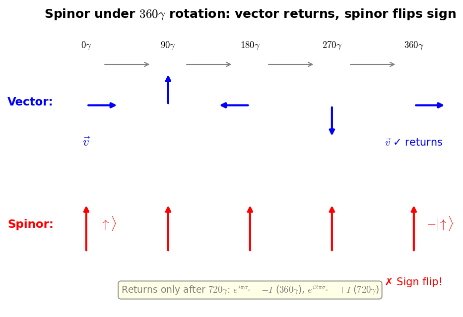
Fig. B.1: Comparison of vector and spinor rotation. A vector returns completely to its original state after \(360°\) rotation, but a spinor's sign flips after \(360°\) rotation (\(-|\!\uparrow\rangle\)), returning to its original state only after \(720°\) rotation. This difference originates from whether the argument of the transformation matrix is \(\theta\) (vector) or \(\theta/2\) (spinor).
✅ Comprehension Check: Find the transformation matrix when a spinor is rotated by \(720°\).
Answer
\(D(4\pi) = I\cos(2\pi) - i\sigma^1\sin(2\pi) = I \cdot 1 - i\sigma^1 \cdot 0 = I\). A \(720°\) rotation returns to the identity matrix.
Spinor Boost—Non-Unitarity
🟡 Lina: After rotations come boosts. For a left-handed Weyl spinor boosted in the \(x^1\) direction, substituting \(\mathbf{K} = -i\boldsymbol{\sigma}/2\) (left-handed) into equation (B.14):
🔵 Kai: For rotations there was \(-i\) multiplying the exponent, but now the \(-i\) cancels with the \(-i\) inside \(K\), making the exponent real.
🟡 Lina: Using \((\sigma^1)^2 = I\) and expanding as in equation (B.30). But this time the exponent is the real number \(-\phi/2\), so instead of \(\cos\) and \(-i\sin\), we get \(\cosh\) and \(-\sinh\). Setting \(\alpha \equiv \phi/2\):
Since \((\sigma^1)^2 = I\), even powers give \(I\) and odd powers give \(\sigma^1\). Collecting even terms: \(\sum_{k=0}^\infty \frac{\alpha^{2k}}{(2k)!}I = I\cosh\alpha\). Collecting odd terms: \(-\sigma^1\sum_{k=0}^\infty \frac{\alpha^{2k+1}}{(2k+1)!} = -\sigma^1\sinh\alpha\). Therefore:
🔵 Kai: For rotations we had \(\cos\) and \(\sin\), but now it's \(\cosh\) and \(\sinh\). Because the exponent became real.
🟡 Lina: Exactly. For rotations the exponent was purely imaginary \(-i\alpha\), giving \(\cos\) and \(\sin\), but now it's real \(-\alpha\), giving \(\cosh\) and \(\sinh\). And there's another important difference. Looking at equation (B.33), \(\cosh(\phi/2)\) is real and \(\sigma^1\) is a Hermitian matrix, so \(D_L\) as a whole is also Hermitian (\(D_L^\dagger = D_L\)). Therefore \(D_L^\dagger D_L = D_L^2\). Using \((\sigma^1)^2 = I\) to compute explicitly:
Expanding gives \((A - B)^2 = A^2 - AB - BA + B^2\). Here \(A = I\cosh(\phi/2)\) is a scalar multiple of the identity, so it commutes with any matrix—meaning \(AB = BA\). So the usual formula \((A-B)^2 = A^2 - 2AB + B^2\) applies directly. \(A^2 = I\cosh^2(\phi/2)\), \(B^2 = (\sigma^1)^2\sinh^2(\phi/2) = I\sinh^2(\phi/2)\), \(2AB = 2\sigma^1\cosh(\phi/2)\sinh(\phi/2)\), so:
⚪ Mei: Using hyperbolic function identities should simplify this.
🟡 Lina: Using the hyperbolic identities \(\cosh^2 x + \sinh^2 x = \cosh 2x\) and \(2\cosh x\sinh x = \sinh 2x\):
So this matrix is not unitary.
🔵 Kai: Not unitary... that means \(D_L^\dagger D_L \neq I\), right? What's wrong with that?
🟡 Lina: Good question. Not being unitary means boosts change the "norm" of spinors. This is connected to a deep property of the Lorentz group. In fact, no non-trivial finite-dimensional unitary representation of the Lorentz group exists. The cause is that the boost generator \(\mathbf{K}\) is anti-Hermitian (\(K^\dagger = -K\), meaning not Hermitian).
Specifically, \(K^i = \pm i\sigma^i/2\) gives \((K^i)^\dagger = (\pm i)^*\sigma^i/2 = \mp i\sigma^i/2 = -K^i\) (since Pauli matrices are Hermitian, \((\sigma^i)^\dagger = \sigma^i\)). So \(K^i\) is anti-Hermitian. Meanwhile, the rotation generator \(J^i = \sigma^i/2\) satisfies \((J^i)^\dagger = \sigma^i/2 = J^i\), which is Hermitian.
🔵 Kai: Rotations are unitary but boosts are non-unitary... But in quantum mechanics, transformations had to be unitary, didn't they?
🟡 Lina: Good question. What must be distinguished here is the difference between operators acting on Hilbert space states and matrices mixing field components. The transformation operators on Hilbert space must be unitary (for probability conservation). However, the finite-dimensional matrices \(D(\Lambda)\) that mix field components need not be unitary. In quantum field theory, this distinction becomes very important.
✅ Comprehension Check: Why doesn't the non-unitarity of the spinor boost transformation matrix contradict probability conservation in quantum mechanics?
Answer
The transformation operators acting on Hilbert space states must be unitary, but the finite-dimensional matrices \(D(\Lambda)\) that mix field components need not be unitary. The non-unitarity of the boost transformation matrix pertains to the mixing of field components, which is a separate matter from probability conservation on the Hilbert space.
Dirac Spinor Transformation
🟡 Lina: Finally, let's look at the transformation of the 4-component Dirac spinor. Stacking the left-handed \(\psi_L\) and right-handed \(\psi_R\) vertically:
Under rotations:
🔵 Kai: The upper-left and lower-right blocks are the same matrix, and left-handed and right-handed don't mix. Does this mean there's no need to distinguish left-handed from right-handed under rotations alone?
🟡 Lina: Exactly. For boosts:
The upper-left and lower-right have opposite signs—this is the difference between left-handed and right-handed. Under rotations there's no distinction, but under boosts the distinction appears—this is the concrete manifestation of the difference between representations \((1/2, 0)\) and \((0, 1/2)\).
⚪ Mei: I see, the sign difference of \(\mathbf{K}\) from the previous section manifests as the sign difference between the upper-left and lower-right blocks of the boost matrix when assembled into 4 components.
🟡 Lina: The transformation matrix for a general Lorentz transformation of spinors can be written using \(\gamma\) matrices as
where \(\sigma^{\mu\nu} = \frac{i}{2}[\gamma^\mu, \gamma^\nu]\) is the generator of Lorentz transformations for the Dirac field. \(\omega_{\mu\nu}\) is the transformation parameter (antisymmetric tensor). This is the true identity of the transformation matrix used in Ch. 5 of the main text.
🔵 Kai: Since \(\sigma^{\mu\nu}\) is constructed from \(4 \times 4\) \(\gamma\) matrices, the transformation matrix for Dirac spinors is also \(4 \times 4\). It's properly extended from the \(2 \times 2\) spin matrices.
✅ Comprehension Check: How many independent components does \(\sigma^{\mu\nu}\) have?
Answer
\(\sigma^{\mu\nu}\) is antisymmetric (\(\sigma^{\mu\nu} = -\sigma^{\nu\mu}\), \(\sigma^{\mu\mu} = 0\)), so the number of independent components is \(4 \times 3/2 = 6\). This matches the number of Lorentz transformation parameters (3 rotations + 3 boosts = 6).
📝 Exercises:
- Computation of \(\sigma^{12} = \frac{i}{2}[\gamma^1, \gamma^2]\) in the Dirac representation → Problem B-7. Calculating Dimensions of Representations
Poincaré Algebra and Particle Classification
🟡 Lina: Adding spacetime translations to Lorentz transformations gives the Poincaré group. Its generators are:
Table B.3: Generators of the Poincaré group and physical quantities
| Transformation | Generator | Physical quantity |
|---|---|---|
| Time translation | \(P^0\) | Energy |
| Spatial translation | \(P^i\) | Momentum |
| Spatial rotation | \(J^i\) | Angular momentum |
| Lorentz boost | \(K^i\) | Boost generator |
The Poincaré algebra commutation relations, in addition to the Lorentz algebra (B.15)–(B.17), are:
An important note here. The \(M^{\mu\nu}\) in this equation is not the anti-Hermitian \(4\times 4\) matrix defined in equation (B.10) itself, but the abstract generator made Hermitian by multiplying by \(-i\). That is:
Using this Hermitian \(M^{\mu\nu}\), we can write simply \(J^i = \frac{1}{2}\varepsilon^{ijk}M^{jk}\), \(K^i = M^{0i}\) (the reason \(-i\) was written explicitly in equation (B.13b) is that there we were using the anti-Hermitian \(M^{jk}\) from equation (B.10)). The values of \(J^i\), \(K^i\) are the same either way.
🔵 Kai: Isn't using the same symbol \(M^{\mu\nu}\) for two meanings confusing?
🟡 Lina: It is indeed confusing. But this is a convention in physics, distinguished by context. Let me organize:
- \(M^{\rho\sigma}\) from equation (B.10): Anti-Hermitian \(4\times 4\) matrices in the vector representation. They appear when writing an infinitesimal transformation as \(\Lambda = I + \omega\), with \(\omega^\mu{}_\nu = \frac{1}{2}\omega_{\rho\sigma}(M^{\rho\sigma})^\mu{}_\nu\)
- \(M^{\mu\nu}\) here: Abstract Hermitian generators, representation-independent. The commutation relation (B.39) uses this meaning
From here on in this chapter, in the context of the Poincaré algebra, \(M^{\mu\nu}\) always refers to the Hermitian version. The commutation relation (B.39) is an abstract algebraic relation that holds independently of any specific representation.
🔵 Kai: Equation (B.38) says "translations commute regardless of order." Walking east first then north, or vice versa, gives the same result.
🟡 Lina: Right. Equation (B.39) states that "\(P^\rho\) transforms as a 4-vector under Lorentz transformations." Intuitively, just as the coordinate \(x^\rho\) changes as \(\delta x^\rho = \omega^\rho{}_\sigma x^\sigma\) under an infinitesimal Lorentz transformation, \(P^\rho\) should mix in the same way—equation (B.39) expresses this "mixing" in the language of commutation relations. The right side \(\eta^{\mu\rho}P^\nu - \eta^{\nu\rho}P^\mu\) has the same structure as the generator \((M^{\mu\nu})^\rho{}_\sigma\) from equation (B.10) acting on \(P^\sigma\) (confirmed by \((M^{\mu\nu})^\rho{}_\sigma P^\sigma = (\eta^{\mu\rho}\delta^\nu{}_\sigma - \eta^{\nu\rho}\delta^\mu{}_\sigma)P^\sigma = \eta^{\mu\rho}P^\nu - \eta^{\nu\rho}P^\mu\)).
⚪ Mei: So (B.39) is the algebraic expression of "\(P^\rho\) behaves as a 4-vector."
🟡 Lina: Let's look at one concrete example. \(M^{12}\) was the rotation generator for the \(xy\) plane (corresponding to \(J^3\)). With \(\rho = 1\):
This means "under rotation about the \(z\)-axis, \(P^1\) (\(x\)-direction momentum) mixes into \(P^2\) (\(y\)-direction momentum)." Just like how vector components mix under rotations.
🔵 Kai: So momentum mixes under rotations just like coordinates do. Then for the commutation relation between the boost generator \(K^i = M^{0i}\) and \(P^\mu\), time and space components would mix?
🟡 Lina: Exactly. Intuitively, just as the coordinate \(x^\rho\) changes as \(\delta x^\rho = \omega^\rho{}_\sigma x^\sigma\) under an infinitesimal Lorentz transformation, \(P^\rho\) also changes as \(\delta P^\rho = \omega^\rho{}_\sigma P^\sigma\)—equation (B.39) expresses this transformation rule in the language of commutation relations. For boosts, the commutator of \(M^{01}\) with \(P^0\) generates \(P^1\)—energy and momentum mix. I'll leave verification of other components as an exercise for you.
Casimir Operators
🟡 Lina: Operators that commute with all generators of the Poincaré algebra are called Casimir operators. There are two for the Poincaré algebra:
Here \(W^\mu\) is called the Pauli-Lubanski vector. Let me explain the motivation. \(P^2\) determines the mass, but where's the spin information? The angular momentum \(M_{\nu\rho}\) itself isn't a Casimir operator (it doesn't commute with \(P^\mu\)). So by combining angular momentum and momentum to "remove the information about the momentum direction," we obtain a new invariant that commutes with all generators. That is:
Here \(\varepsilon^{\mu\nu\rho\sigma}\) is the 4-dimensional Levi-Civita symbol—the 4-dimensional extension of the 3-dimensional \(\varepsilon^{ijk}\) used in equation (B.13), with \(\varepsilon^{0123} = +1\), \(+1\) for even permutations, \(-1\) for odd permutations, and \(0\) if any indices repeat. Intuitively, \(W^\mu\) is a quantity that subtracts the "orbital motion contribution" from angular momentum to extract pure spin information. Let's see this concretely.
🔵 Kai: In natural units, \(P^2 = -(P^0)^2 + |\mathbf{p}|^2 = -E^2 + |\mathbf{p}|^2 = -m^2\), right? This determines the particle's mass.
🟡 Lina: Exactly. For \(W^2\), it's easiest to consider a massive particle (\(m > 0\)) in its rest frame. In the rest frame \(P^\mu = (m, 0, 0, 0)\), so only \(P_0 = \eta_{00}P^0 = -m\) is non-zero (\(P_i = 0\)). Substituting into equation (B.42):
For \(\mu = 0\): \(\varepsilon^{0\nu\rho 0} = 0\) (the index \(0\) appears twice), so \(W^0 = 0\). For \(\mu = i\) (spatial components), let's systematically find the values of \(\varepsilon^{i\nu\rho 0}\). Since \(\varepsilon^{\mu\nu\rho\sigma}\) is totally antisymmetric with \(\varepsilon^{0123} = +1\), let's find \(\varepsilon^{1230}\) as an example. Totally antisymmetric means "the sign flips with each swap of any two indices." Starting from \(\varepsilon^{0123} = +1\), let's move \(0\) to the rightmost position. \((0,1,2,3) \to (1,0,2,3)\) (swap 1st and 2nd indices, sign \(\times(-1)\)) \(\to (1,2,0,3)\) (swap 2nd and 3rd indices, sign \(\times(-1)\)) \(\to (1,2,3,0)\) (swap 3rd and 4th indices, sign \(\times(-1)\)). Three adjacent swaps give a sign of \((-1)^3 = -1\), so \(\varepsilon^{1230} = -1\). In general, \(\varepsilon^{ijk0} = -\varepsilon^{ijk}\) holds. Here the right side \(\varepsilon^{ijk}\) is the 3-dimensional Levi-Civita symbol (\(\varepsilon^{123} = +1\), \(+1\) for even permutations, \(-1\) for odd). This relation follows from "moving \(0\) from the front to the back in 4-dimensional \(\varepsilon^{ijk0}\) requires 3 adjacent swaps, and an odd number means the sign flips."
🔵 Kai: I see, moving \(0\) from the front to the back requires 3 swaps, producing a minus sign.
🟡 Lina: Therefore:
Here \(\nu, \rho\) run over \(0, 1, 2, 3\), but \(\varepsilon^{i\nu\rho 0}\) is non-zero only when all four indices \(i, \nu, \rho, 0\) are different. Since \(0\) already occupies the 4th position, \(\nu\) and \(\rho\) must be spatial indices \(j, k\) (not \(0\)). Therefore:
⚪ Mei: The two minuses cancel to give a clean form.
🟡 Lina: Now, the definition \(J^i = \frac{1}{2}\varepsilon^{ijk}M^{jk}\) is written with upper indices \(M^{jk}\), so we want to convert \(M_{jk}\) to \(M^{jk}\). For spatial indices, raising and lowering involves \(\eta_{jk} = +\delta_{jk}\) (the spatial part is just the Euclidean metric), so \(M_{jk} = \eta_{ja}\eta_{kb}M^{ab} = \delta_{ja}\delta_{kb}M^{ab} = M^{jk}\)—spatial indices have the same value whether up or down (only the time index gets a sign change from \(\eta_{00} = -1\)). Here \(M^{jk}\) is the Hermitian generator introduced at the beginning of this section, for which \(J^i = \frac{1}{2}\varepsilon^{ijk}M^{jk}\) holds simply. Using this relation:
In the rest frame \(W^0 = 0\), so using \(W^i = mJ^i\) to compute \(W^2\): \(W^2 \equiv W_\mu W^\mu = \eta_{\mu\nu}W^\mu W^\nu\), with the sign convention \(\eta_{\mu\nu} = \mathrm{diag}(-1,+1,+1,+1)\):
Substituting \(W^0 = 0\):
The eigenvalue of \(\mathbf{J}^2\) is \(s(s+1)\) where \(s\) is the spin quantum number (we're using natural units \(\hbar = 1\); restoring \(\hbar\) gives \(\hbar^2 s(s+1)\)), so:
where \(s\) is the spin quantum number.
🔵 Kai: Oh, the square of the Pauli-Lubanski vector equals the product of mass and spin!
⚪ Mei: So particles are completely classified by the eigenvalues of the two Casimir operators—mass \(m\) and spin \(s\).
🟡 Lina: Exactly. This is the complete list of particle classification derived from Poincaré invariance alone.
Table B.4: Classification of particles by mass and spin
| Mass | Spin | Examples |
|---|---|---|
| \(m > 0\) | \(s = 0\) | Higgs boson |
| \(m > 0\) | \(s = 1/2\) | Electron, quarks |
| \(m > 0\) | \(s = 1\) | \(W\) boson, \(Z\) boson |
| \(m = 0\) | Helicity \(\pm 1\) | Photon |
| \(m = 0\) | Helicity \(\pm 2\) | Graviton (hypothetical) |
⚪ Mei: So \(P^2\) determines the mass, \(W^2\) determines the spin, and particles are completely classified by just these two quantum numbers.
🔵 Kai: Symmetry alone constrains what kinds of particles can exist to this extent... "Invariance determines physics" is really true. But one thing I'm curious about—why are massless particles classified by "helicity" instead of "spin"?
🟡 Lina: Good question. Massless particles travel at the speed of light, so no rest frame exists. Without a rest frame, the structure of the Pauli-Lubanski vector changes, and instead of spin, only helicity (the projection of angular momentum onto the direction of motion) remains as a good quantum number. This was discussed in detail in Ch. 4 of the main text.
✅ Comprehension Check: Briefly explain why massless particles are classified by helicity rather than spin.
Answer
Massless particles travel at the speed of light, so no rest frame exists. Without a rest frame, the structure of the Pauli-Lubanski vector changes, and instead of all components of spin, only helicity—the projection of angular momentum onto the direction of motion—remains as a good quantum number.
🟡 Lina: This is the mathematical culmination of the philosophy running through the entire Quantum Field Theory. The individual field equations (Klein-Gordon, Dirac, Maxwell) merely describe fields corresponding to specific representations of the Poincaré group.
✅ Comprehension Check: What are the two Casimir operators of the Poincaré group? State the physical meaning of each.
Answer
\(C_1 = P^2 = P_\mu P^\mu\) (eigenvalue is \(-m^2\), determines the square of the particle's mass; with metric \((-,+,+,+)\), \(P^2 = -(P^0)^2 + |\mathbf{p}|^2 = -m^2\)) and \(C_2 = W^2 = W_\mu W^\mu\) (eigenvalue is \(m^2 s(s+1)\), determines the particle's spin).
Summary—What This Appendix Achieved
🟡 Lina: Let's organize what we've accomplished in this Appendix.
- Generators and exponential map: From infinitesimal transformation generators, finite transformations are constructed via the exponential \(e^{\pm i\alpha G}\) (sign is convention-dependent)
- Lorentz algebra: The commutation relations (B.15)–(B.17) of rotation generators \(J^i\) and boost generators \(K^i\) completely determine the infinitesimal structure of the Lorentz group
- \(\mathfrak{su}(2) \oplus \mathfrak{su}(2)\) decomposition: By introducing \(\mathbf{J}_\pm = (\mathbf{J} \pm i\mathbf{K})/2\), the Lorentz algebra decomposes into two independent \(\mathfrak{su}(2)\)'s
- Classification of representations: Field types are determined by the pair \((j_+, j_-)\)—scalar \((0,0)\), Weyl spinor \((1/2, 0)\) and \((0, 1/2)\), vector \((1/2, 1/2)\)
- Spinor construction: Transformation matrices for rotations and boosts were explicitly constructed from Pauli matrices. The origin of the sign-flip property under \(360°\) rotation traces back to the generator being \(\boldsymbol{\sigma}/2\) (argument is \(\theta/2\))
- Poincaré algebra and particle classification: The eigenvalues of two Casimir operators (\(P^2\) and \(W^2\)) determine mass and spin, completely classifying particles in nature
🔵 Kai: It's truly amazing that the mathematics of symmetry determines all the types of particles.
⚪ Mei: So there's no need to memorize individual field equations—the moment you choose \((j_+, j_-)\), the transformation properties of the field are determined, and from there the form of the equation is constrained. The structure is "symmetry first," not "equation first."
🟡 Lina: Exactly. This is at the heart of the beauty of quantum field theory.
Preview of Next Chapter
Appendix C: Gaussian Integrals and Grassmann Integrals
We compile in one place the Gaussian integrals (the foundation of bosonic path integrals) and Grassmann number algebra/Berezin integration (the foundation of fermionic path integrals) that appear repeatedly in quantum field theory calculations. Once you grasp the contrast between the bosonic \((\det A)^{-1/2}\) and the fermionic \(\det A\), the difference in how the two types of particles are handled in path integrals becomes clear. The subsequent Appendix D "Toolbox for Loop Calculations" then proceeds to practical techniques for loop integrals: dimensional analysis, Feynman parameters, Wick rotation, and more.
Exercises
📝 Exercises:
- Verification of \([K^i, K^j] = -i\varepsilon^{ijk}J^k\) in the vector representation → Problem M-3. Correspondence Between the \((1/2, 1/2)\) Representation and 4-Vectors
- Re-derivation of Lorentz algebra from \(\mathbf{J}_\pm\) → Problem B-5. Recovering Rotation Generators Using the Levi-Civita Symbol
- Confirmation of \(\mathbf{J}_\pm\) and representation \((0, 1/2)\) for right-handed Weyl spinors → Problem B-6. Expressing \(\mathbf{J}\) and \(\mathbf{K}\) in terms of \(\mathbf{J}_+\) and \(\mathbf{J}_-\)
- Computation of \(\sigma^{12} = \frac{i}{2}[\gamma^1, \gamma^2]\) in the Dirac representation → Problem B-7. Calculating Dimensions of Representations
References
- Quantum Field Theory for the Gifted Amateur (Lancaster & Blundell) Chapter 10 "Transformations," Chapter 37 "Spinor Transformations"
- 坂本眞人『場の量子論 — 不変性と自由場を中心にして』 Chapter 5 "Relativistic Structure of the Dirac Equation," Chapter 14 "Poincaré Algebra and Classification of One-Particle States"
- Quantum Field Theory and the Standard Model (Schwartz) Chapter 8 "Spinors and the Dirac equation"
- Quantum Field Theory (Tong) Chapter 4 "Lorentz group representations and spinors"
Feedback on this page
Let us know if something was unclear, incorrect, or could be improved.