Appendix C: The Field Lagrangian and Euler–Lagrange Equations
Story so far: In Appendix B, we learned the definition and algebraic rules of the tensor product \(\otimes\) and understood the structure of the contravariant tensor space \(T^r(V)\). We introduced Einstein's summation convention and confirmed the correspondence between component representation of tensors and their interpretation as multilinear maps. With these tools in hand, we are now prepared to write down field equations in component form. In this chapter, we make use of that component notation as we proceed to the action principle for fields and the derivation of equations of motion. Note that from C.6 onward, we will also use the knowledge of covariant derivatives learned in Ch. 12. The principle of least action (Ch. 1) serves as the foundation throughout the entire chapter.
Goals of this chapter
- Extend the particle action principle to fields
- Introduce the concept of Lagrangian density and derive the field Euler–Lagrange equations
- Furthermore, learn how to write field actions in curved spacetime and outline the path to the Einstein–Hilbert action
C.1: Why Do We Need an Action Principle for "Fields"?
🟡 Lina: In Ch. 1, we derived the equations of motion for a particle from the principle of least action. Back then, the dynamical variables were "the particle's position \(x^i(t)\)"—just a finite number of functions of time.
We added a small displacement \(\delta x^i\) (dashed line) around the actual path (solid line) and found the condition for the action to be extremal (Fig. C.1 "Figure C.1: The concept of the variational method"). In field theory, this \(\delta x^i\) gets replaced by a small displacement \(\delta\phi\) of the field—that's the theme of this chapter.
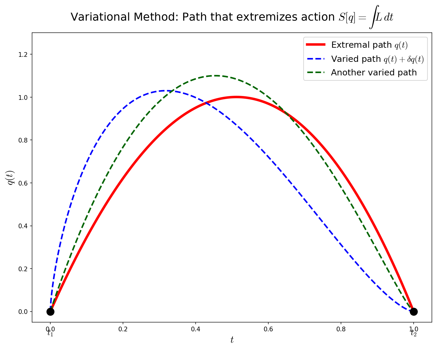
Fig. C.1: Figure C.1: The concept of the variational method. A small displacement (dashed line) is added around the actual configuration (solid line), and we find the condition for the action to be extremal. In particle mechanics, \(\delta x^i\) corresponds to this displacement; in field theory, it is \(\delta\phi\).
🔵 Kai: Right. In 3D space, there are just the three functions \(x^1(t), x^2(t), x^3(t)\).
🟡 Lina: But what was the protagonist of general relativity?
🔵 Kai: Um... the metric?
🟡 Lina: Yes, the metric field \(g_{\mu\nu}(x)\). This isn't "a finite number of coordinates"—it has a value attached to every point of spacetime. That means we have infinitely many dynamical variables. We can't just use the particle action principle as-is—we need to extend it for field theory.
🔵 Kai: In the particle case, we "slightly shifted the path and found the condition for the action to be extremal." What about for fields?
🟡 Lina: We "slightly shift the field value at each point and find the condition for the action to be extremal." The spirit is exactly the same. The only difference is that the integral now extends over all of spacetime, not just over time.
✅ Comprehension Check: What is the essential difference between the action principle for particles and the action principle for fields?
Answer
In the particle case, the dynamical variables are a finite number of coordinates \(x^i(t)\), and the action is an integral over time only. In the field case, the dynamical variables are fields \(\phi(x^\mu)\) that have values at every spacetime point (infinitely many degrees of freedom), and the action is an integral over all of spacetime. However, the spirit of "taking variations and finding the extremal condition" remains the same.
C.2: From Particles to Fields—The Correspondence
🟡 Lina: First, let's organize the correspondence between particle mechanics and field theory (Table C.1 "Correspondence between particle mechanics and field theory").
Table C.1: Correspondence between particle mechanics and field theory
| Particle mechanics | Field theory |
|---|---|
| Generalized coordinate \(q(t)\) | Field \(\phi(x^\mu)\) |
| Generalized velocity \(\dot{q}\) | Field derivative \(\partial_\mu \phi\) |
| Lagrangian \(L(q, \dot{q})\) | Lagrangian density \(\mathcal{L}(\phi, \partial_\mu \phi)\) |
| Action \(S = \int dt \, L\) | Action \(S = \int d^4x \, \mathcal{L}\) |
⚪ Mei: The discrete index \(i\) (the coordinate label) gets replaced by the continuous spacetime coordinate \(x^\mu\).
🔵 Kai: What's \(d^4x\)?
🟡 Lina: It's the volume element of 4-dimensional spacetime. \(d^4x = dt\,dx\,dy\,dz\). The field's Lagrangian density \(\mathcal{L}\) is the "Lagrangian per unit volume," so integrating over all space gives the total Lagrangian \(L\):
If we also integrate over time, we get the action \(S\):
⚪ Mei: That's why \(\mathcal{L}\) is called the "Lagrangian density." Since it's a density, integrating gives the total quantity.
✅ Comprehension Check: State the relationship between the Lagrangian density \(\mathcal{L}\), the Lagrangian \(L\), and the action \(S\).
Answer
The Lagrangian density \(\mathcal{L}\) is the Lagrangian per unit volume. Integrating over all space gives the Lagrangian \(L = \int d^3x\,\mathcal{L}\). Integrating further over time yields the action \(S = \int d^4x\,\mathcal{L}\).
C.3: Building Intuition with a Concrete Example—Vibrating String
🟡 Lina: Before getting into abstractions, let's build intuition with an example familiar even from high school. Consider a string with tension \(\mathcal{T}\) and linear mass density \(\rho\). Let the displacement of each point on the string be \(\psi(x,t)\).
🔵 Kai: Like a guitar string, right?
🟡 Lina: Exactly. The Lagrangian density for this system is:
🔵 Kai: \(\frac{\partial \psi}{\partial t}\) is the velocity of each point on the string, so \(\frac{1}{2}\rho v^2\) is the kinetic energy density... that makes sense. But why is the second term \(\left(\frac{\partial\psi}{\partial x}\right)^2\)? I don't see why the square of the slope gives energy.
🟡 Lina: Good question. Where the string is tilted, it's stretched compared to being horizontal—the tension \(\mathcal{T}\) does work against that stretching, so energy is stored. The actual length of a small segment \(dx\) of the string is \(\sqrt{1 + (\partial_x\psi)^2}\,dx \approx (1 + \frac{1}{2}(\partial_x\psi)^2)\,dx\), so the amount of stretching is proportional to \(\frac{1}{2}(\partial_x\psi)^2\,dx\). Multiplying by the tension gives the energy density \(\frac{\mathcal{T}}{2}(\partial_x\psi)^2\).
🟡 Lina: The key point of this example is that the dynamical variable is a field \(\psi(x,t)\). Each point \(x\) on the string plays the role of a "generalized coordinate index," giving us continuously infinitely many dynamical variables.
✅ Comprehension Check: In the vibrating string example, what concept in particle mechanics does each point \(x\) on the string correspond to?
Answer
Each point \(x\) on the string corresponds to the "index" (discrete label \(i\)) of generalized coordinates in particle mechanics. While particle mechanics has a finite number of coordinates \(q_i(t)\), the string has a displacement \(\psi(x,t)\) for each continuous position \(x\), giving continuously infinitely many dynamical variables.
📝 Exercises:
- Partial derivatives of the string Lagrangian density → Problem B-3. Partial Derivatives of the String Lagrangian
C.4: Deriving the Field Euler–Lagrange Equation
🟡 Lina: Now for the main event. When the action for a scalar field \(\phi(x^\mu)\) is given by
let's derive the equation of motion from \(\delta S = 0\).
Step 1: Variation of the Field
🟡 Lina: We shift the field by a small amount:
As a boundary condition, we require \(\delta\phi = 0\) on the boundary of the integration region \(D\). This is the same spirit as setting \(\delta x^i = 0\) at the endpoints in the particle case.
Step 2: Computing the Variation of the Action
🟡 Lina: The first-order change in the action is:
This uses the same idea as the total differential of a multivariable function. Since \(\mathcal{L}\) depends on two types of variables, \(\phi\) and \(\partial_\mu\phi\), we add the contribution from \(\phi\) changing by \(\delta\phi\) and the contribution from \(\partial_\mu\phi\) changing—an extension of \(df = \frac{\partial f}{\partial x}dx + \frac{\partial f}{\partial y}dy\) from high school. The notation \(\frac{\partial\mathcal{L}}{\partial(\partial_\mu\phi)}\) means "differentiate with respect to \(\partial_\mu\phi\), treating it as independent of \(\phi\)"—the same idea as computing \(\frac{\partial L}{\partial\dot{q}}\) in particle mechanics by treating \(q\) and \(\dot{q}\) as separate variables. I'll show the concrete calculation method step by step in C.5, so for now just think of it as "this notation exists."
⚪ Mei: The correspondence \(q \to \phi\), \(\dot{q} \to \partial_\mu\phi\) from the table in C.2 (Table C.1 "Correspondence between particle mechanics and field theory") is showing up directly in this expression.
🟡 Lina: Exactly. You can see the terms corresponding to \(q \to \phi\) and \(\dot{q} \to \partial_\mu \phi\) lined up respectively.
🔵 Kai: What's \(\delta(\partial_\mu \phi)\)?
🟡 Lina: The bottom line is that the variation and partial derivative commute, so \(\delta(\partial_\mu \phi) = \partial_\mu(\delta\phi)\).
🔵 Kai: Wait, you can swap the order? Why?
🟡 Lina: Intuitively, \(\delta\phi\) is a "small displacement of the field"—it changes the field value at each point \(x^\mu\) slightly, but doesn't shift the coordinate \(x^\mu\) itself—the same spirit as changing the shape of the path while keeping the endpoints fixed in particle mechanics. So the operation of differentiating with respect to \(x^\mu\) (\(\partial_\mu\)) and the operation of shifting the field value (\(\delta\)) don't interfere with each other—"shift then differentiate" gives the same result as "differentiate then shift."
🔵 Kai: So because the coordinates are fixed and only the field values move, the partial derivative and variation don't interfere... is that right?
🟡 Lina: Exactly. The operation of differentiating with respect to coordinates and the operation of shifting field values are independent, so they commute. Let me verify this more concretely. The definition of \(\partial_\mu\phi\) is "the rate of change of \(\phi\) when you advance by a small amount \(\epsilon\) in the \(x^\mu\) direction," i.e.:
When the field is shifted \(\phi \to \phi + \delta\phi\), every \(\phi\) in this definition is simply replaced by \(\phi + \delta\phi\), so the change is:
So \(\delta(\partial_\mu\phi) = \partial_\mu(\delta\phi)\) holds.
🔵 Kai: Oh, if you just go back to the definition and write it out, it comes out directly. That's satisfying.
Step 3: Integration by Parts
🟡 Lina: We apply integration by parts to the second term. The idea is exactly the same as in the particle case. Since \(\partial_\mu\) is an ordinary partial derivative with respect to \(x^\mu\), the product rule from high school applies directly. Writing the 4-dimensional version of \(f\,g' = (fg)' - f'\,g\):
🔵 Kai: Setting \(f = \frac{\partial\mathcal{L}}{\partial(\partial_\mu\phi)}\) and \(g = \delta\phi\), you used \((fg)' = f'g + fg'\) and moved \(fg'\) to the left side!
🟡 Lina: Exactly. The first term is a total divergence—it has the form \(\partial_\mu(\text{something})\). When you integrate such a term over all space, Gauss's theorem (the divergence theorem) converts it into a surface integral over the boundary.
🔵 Kai: The divergence theorem—is that the one from high school that "converts a volume integral into a surface integral"?
🟡 Lina: Yes, its generalization. In 1D, \(\int_a^b f'(x)\,dx = f(b) - f(a)\)—integrating a derivative leaves only the boundary values. In 3D, a volume integral becomes a boundary surface integral. In 4D, exactly the same principle applies: a 4-dimensional volume integral becomes a 3-dimensional boundary integral. In equation form: \(\int_D \partial_\mu V^\mu\,d^4x = \oint_{\partial D} V^\mu\,dS_\mu\)—the left-hand side "integral of the divergence inside" equals the right-hand side "integral over the boundary surface." Here \(dS_\mu\) is the "oriented surface element" of the boundary—think of it as the 4-dimensional version of the normal vector \(\vec{n}\,dA\) that appears in surface integrals in the 3D divergence theorem.
🔵 Kai: A 4-dimensional surface element is honestly hard to picture, but... can I just think of it as the same spirit as the 1D case where "only boundary values remain"?
🟡 Lina: That understanding is sufficient. In our case, we're setting \(V^\mu = \frac{\partial\mathcal{L}}{\partial(\partial_\mu\phi)}\,\delta\phi\). The quantity \(\frac{\partial\mathcal{L}}{\partial(\partial_\mu\phi)}\) gives one number for each value of \(\mu\)—meaning it has 4 components, and multiplying by \(\delta\phi\) (a scalar) keeps it at 4 components. So \(V^\mu\) can play the role of a "4-component vector-like quantity" appearing in the divergence theorem. Since we assumed \(\delta\phi = 0\) on the boundary \(\partial D\), \(V^\mu\) is also zero on the boundary—therefore the right-hand side vanishes. This term drops out.
⚪ Mei: In particle mechanics too, we set \(\delta q = 0\) at the endpoints to eliminate boundary terms—the exact same argument has just been extended to 4 dimensions.
Step 4: The Euler–Lagrange Equation
🟡 Lina: Collecting what remains:
This must be zero for arbitrary \(\delta\phi(x)\). If the bracketed expression were positive (for example) at some point \(x_0\), then by continuity it would remain positive in a neighborhood of \(x_0\). We could then choose a \(\delta\phi\) that is positive only near \(x_0\) and zero elsewhere, making the integral positive—contradicting \(\delta S = 0\).
🔵 Kai: Can you really construct a function that's "positive only near \(x_0\) and zero elsewhere"? You also need to satisfy \(\delta\phi = 0\) on the boundary...
🟡 Lina: You can. For example, it's known that there exist functions that smoothly rise only inside a small ball centered at \(x_0\) and are exactly zero outside the ball. In mathematics, such functions are called "functions with compact support"—"support" means the region where the function is nonzero, and "compact" roughly means that region is contained within a finite extent (doesn't extend to infinity). Since the boundary is the edge of the integration region, as long as \(x_0\) is in the interior, making the ball sufficiently small avoids any conflict with boundary conditions.
🔵 Kai: I see—you can place such a "test function" anywhere in the interior, so there's no escape.
🟡 Lina: Right. So the bracketed expression must be zero at every point:
This is the field Euler–Lagrange equation.
⚪ Mei: The correspondence \(q \to \phi\), \(\dot{q} \to \partial_\mu\phi\) from the table in C.2 (Table C.1 "Correspondence between particle mechanics and field theory") is directly reflected here—the structure is completely parallel to the particle case.
🔵 Kai: The structure is the same, so it's easy to remember! But \(\partial_\mu\) means a sum over \(\mu = 0,1,2,3\), right? What does it look like when you actually compute it...?
🟡 Lina: Good question. Let's work it out in the next section.
📝 Exercises:
- Computing \(\partial\mathcal{L}/\partial\phi\) → Problem B-1. Klein-Gordon \(\partial \mathcal{L}/\partial \phi\), Computing \(\partial\mathcal{L}/\partial(\partial_\mu\phi)\) → Problem B-2. Klein-Gordon \(\partial \mathcal{L}/\partial(\partial\phi)\), Partial derivatives for \(\phi^4\) theory → Problem B-4. \(\partial \mathcal{L}/\partial \phi\) in \(\phi^4\) Theory, 2D Euler–Lagrange equation → Problem B-6. Euler–Lagrange Equation for a 2-Dimensional Scalar Field
C.5: Concrete Example—Equation of Motion for a Free Scalar Field
🟡 Lina: Let's use the equation we derived to obtain a concrete equation of motion. The Lagrangian density for a free scalar field in 4-dimensional Minkowski spacetime—"free" meaning no interactions with other fields, i.e., a system closed in \(\phi\) alone—is:
You might be surprised by the overall minus sign, but this is designed so that when expanded, the time-derivative term becomes positive due to \(\eta^{00} = -1\)—I'll verify this shortly. First, let me explain where this expression comes from. It's obtained by extending the string's Lagrangian density \(\frac{\rho}{2}(\partial_t\psi)^2 - \frac{\mathcal{T}}{2}(\partial_x\psi)^2\) from C.3 to 4 dimensions, and writing it in a Lorentz-invariant form—meaning the expression doesn't change its form under special-relativistic coordinate transformations (Lorentz transformations). For the string, time and space derivatives were written separately, but using \(\eta^{\mu\nu}\) lets us combine time and space into a single expression. Why is it Lorentz invariant? Because \(\eta^{\mu\nu}(\partial_\mu\phi)(\partial_\nu\phi)\) is a scalar quantity with all indices contracted—each component changes under Lorentz transformations, but the result of contraction (the summing operation) doesn't change. It's exactly the same principle as how the dot product \(\vec{a}\cdot\vec{b}\) is invariant under rotations.
🔵 Kai: Ah, it uses the same mechanism as the invariance of inner products. Then what about the \(-\frac{m^2}{2}\phi^2\) part?
🟡 Lina: \(-\frac{m^2}{2}\phi^2\) is a mass term that wasn't present for the string—why it's called "mass" is because if you substitute a plane wave solution \(\phi \propto e^{i(\vec{k}\cdot\vec{x} - \omega t)}\)—the complex exponential wave notation learned in Appendix A—into the equation of motion derived from this Lagrangian (which we'll derive shortly), you get the dispersion relation \(\omega^2 = |\vec{k}|^2 + m^2\). This has the same form as the relativistic energy-momentum relation \(E^2 = |\vec{p}|^2 + m^2\) (which we learned in Ch. 4). So \(m\) is a parameter corresponding to the rest mass of the field's quanta (particles). I'll explain why this is so after we derive the Klein–Gordon equation at the end of this section. For now, it's enough to think of it as "a heaviness parameter—the larger \(m\) is, the harder it is for the field to oscillate."
⚪ Mei: So the \(\eta^{\mu\nu}\) term is the relativistic packaging of the string's "\(T - V\)," and the \(m^2\) term is an additional potential due to mass.
🟡 Lina: Here \(\eta^{\mu\nu}\) is the inverse of the Minkowski metric \(\eta_{\mu\nu} = \mathrm{diag}(-1,+1,+1,+1)\). The inverse of a diagonal matrix has the reciprocal of each entry, so \(1/(-1) = -1\), \(1/1 = 1\), giving \(\eta^{\mu\nu} = \mathrm{diag}(-1,+1,+1,+1)\)—the components are the same. Note that we're using natural units (\(c = \hbar = 1\)) here. \(c = 1\) is the unit system introduced in Ch. 4—making distance and time have the same dimensions. Here we additionally set \(\hbar = 1\) (Planck's constant equals 1), unifying the dimensions of energy, mass, inverse length, and inverse time (see Ch. 25 for details). This makes equations concise, but when you want to restore original units, you need to use dimensional analysis to put \(c\) and \(\hbar\) back in the appropriate places.
🔵 Kai: If \(c = \hbar = 1\), what are the dimensions of \(m\) in this expression?
🟡 Lina: With \(c = \hbar = 1\), mass, energy, momentum, inverse length, and inverse time all have the same dimensions—as we confirmed in Ch. 25. So \(m\) appearing in the Klein–Gordon equation has dimensions of "inverse length"—the larger \(m\) is, the shorter the Compton wavelength \(1/m\) becomes.
🔵 Kai: Wait, there's an overall minus sign, but for the string it was \(+\frac{\rho}{2}(\dot\psi)^2 - \cdots\), right? Does it really become positive when expanded?
🟡 Lina: Let's check. Since the time component of \(\eta^{\mu\nu}\) is \(\eta^{00} = -1\), the \(\mu=\nu=0\) term of \(-\frac{1}{2}\eta^{\mu\nu}(\partial_\mu\phi)(\partial_\nu\phi)\) is \(-\frac{1}{2}\times(-1)\times(\partial_t\phi)^2 = +\frac{1}{2}(\partial_t\phi)^2\). See—the two minuses cancel and it becomes positive. The mass term \(-\frac{m^2}{2}\phi^2\) is also the "\(-V\)" part of the Lagrangian's "\(T - V\)" structure—a potential energy density \(V = \frac{m^2}{2}\phi^2 \geq 0\) with a minus sign in front.
🔵 Kai: What happens when you expand using \(\eta^{\mu\nu}\)?
🟡 Lina: Since \(\eta^{\mu\nu} = \mathrm{diag}(-1,+1,+1,+1)\), only the diagonal components survive. Let me expand it:
Substituting the values of each component:
Here \((\nabla\phi)^2 = (\partial_x\phi)^2 + (\partial_y\phi)^2 + (\partial_z\phi)^2\) is the sum of squares of spatial derivatives. Combining with the preceding \(-\frac{1}{2}\):
Adding the mass term:
⚪ Mei: The first term is "kinetic energy density," and the rest is "potential energy density." The same \(T - V\) structure as the string.
🟡 Lina: Now let's compute the Euler–Lagrange equation.
Step 1: Partial derivative with respect to \(\phi\):
Step 2: Partial derivative with respect to \(\partial_\mu \phi\). Let me state the final result first:
🟡 Lina: I'll derive "why this is so" step by step below, so first let me confirm how to read this expression. In the right-hand side, \(\nu\) appears in both \(\eta^{\mu\nu}\) (upper index) and \(\partial_\nu\phi\) (lower index)—by Einstein's summation convention learned in Appendix B, when the same index appears once up and once down, we sum over \(\nu = 0,1,2,3\). So \(\nu\) is a "dummy index" (summed over). Meanwhile, \(\mu\) appears only once on each side—it's a "free index" that isn't summed. For each fixed value of \(\mu\), we get one equation, so this expression represents 4 equations in total.
🔵 Kai: Why does \(\eta^{\mu\nu}\partial_\nu\phi\) appear? In the first place, what does it mean to differentiate with respect to \(\partial_\mu\phi\)—what's held fixed and what's varied?
🟡 Lina: The key point here is treating \(\partial_\mu\phi\) as an independent variable. Remember—in particle mechanics with the Lagrangian \(L(q, \dot{q})\), although \(q\) and \(\dot{q}\) are physically "\(q\) differentiated with respect to time," when computing partial derivatives we treated them as formally separate variables. When computing \(\frac{\partial L}{\partial q}\), we hold \(\dot{q}\) fixed; when computing \(\frac{\partial L}{\partial \dot{q}}\), we hold \(q\) fixed. Why? Because we view the Lagrangian as "a function with two input slots, \(q\) and \(\dot{q}\)." On physical trajectories, the relation \(\dot{q} = dq/dt\) holds, but at the stage of computing partial derivatives, we're asking "if only \(\dot{q}\) changes while \(q\) is fixed, how does \(L\) change?"—imposing the constraint of actual motion comes after computing the partial derivatives.
🔵 Kai: Ah right, in the particle case we also treated \(q\) and \(\dot{q}\) as "separate things." So for fields, the same idea applies—we treat \(\phi\) and \(\partial_0\phi, \partial_1\phi, \partial_2\phi, \partial_3\phi\) as separate variables?
🟡 Lina: Exactly. We treat all 5 as formally independent variables. It's the same idea as in an ordinary multivariable function \(f(u, v, w)\) where \(\frac{\partial u}{\partial v} = 0\)—if \(u, v, w\) are independent variables, varying \(v\) doesn't change \(u\). Here \(\phi, \partial_0\phi, \partial_1\phi, \partial_2\phi, \partial_3\phi\) correspond to those "independent variables." So \(\frac{\partial(\partial_\alpha\phi)}{\partial(\partial_\mu\phi)} = \delta^\mu{}_\alpha\). The symbol \(\delta^\mu{}_\alpha\) is the Kronecker delta—it equals 1 when \(\alpha = \mu\) and 0 otherwise (it also appeared in Ch. 6 and Appendix B). The upper and lower placement of indices is a notational convention; here it simply functions as a symbol that "checks whether \(\alpha\) and \(\mu\) have the same value." It's exactly the same idea as writing \(\frac{\partial x_i}{\partial x_j} = \delta_{ij}\) (\(= 1\) if \(i = j\), \(= 0\) if \(i \neq j\)) for ordinary multivariable functions—just with indices split between upper and lower positions. For example, fixing \(\mu = 1\): \(\frac{\partial(\partial_1\phi)}{\partial(\partial_1\phi)} = 1\), but \(\frac{\partial(\partial_0\phi)}{\partial(\partial_1\phi)} = 0\)—since \(\partial_0\phi\) and \(\partial_1\phi\) are independent variables, differentiating with respect to one doesn't affect the other.
⚪ Mei: The Kronecker delta serves as a "filter for whether it's the same variable."
🟡 Lina: Note that the mass term \(-\frac{m^2}{2}\phi^2\) doesn't contain \(\partial_\mu\phi\), so differentiating with respect to \(\partial_\mu\phi\) gives zero—only the kinetic term \(-\frac{1}{2}\eta^{\alpha\beta}(\partial_\alpha\phi)(\partial_\beta\phi)\) contributes. Here I've relabeled the dummy indices from the original expression's \(\mu, \nu\) to \(\alpha, \beta\) to avoid collision with the index \(\mu\) of the variable we're differentiating with respect to—since dummy indices are "disposable letters for summing," changing their names doesn't change the physical meaning.
Now, in the definition of \(\mathcal{L}\), we wrote \(\eta^{\mu\nu}(\partial_\mu\phi)(\partial_\nu\phi)\), where \(\mu, \nu\) were dummy indices (indices for summing). But now when we say "differentiate with respect to \(\partial_\mu\phi\)," that \(\mu\) is a free index—representing a fixed value. Using the same letter for two different meanings would be confusing, so I'll relabel the dummy indices in the Lagrangian density to \(\alpha, \beta\). The expression \(\eta^{\alpha\beta}(\partial_\alpha\phi)(\partial_\beta\phi)\) is exactly the same quantity as the original \(\eta^{\mu\nu}(\partial_\mu\phi)(\partial_\nu\phi)\)—we've only changed letters. This way, the index \(\mu\) of the differentiation variable won't collide with the summation indices.
🔵 Kai: So you change letters to avoid index collision. Since the content is the same, no worries...
🟡 Lina: Now I'll differentiate this with respect to \(\partial_\mu \phi\). Here \(\eta^{\alpha\beta}(\partial_\alpha\phi)(\partial_\beta\phi)\) is a double sum over \(\alpha, \beta\) each running from \(0,1,2,3\), so expanding gives a quadratic expression in the 4 independent variables \(\partial_0\phi, \partial_1\phi, \partial_2\phi, \partial_3\phi\). For example, if differentiating with \(\mu = 1\), "only terms containing \(\partial_1\phi\) survive." The \(\eta^{\alpha\beta}\) are components of the Minkowski metric and are constants independent of \(\partial_\mu\phi\), so they can be taken outside the derivative—just like \(\frac{d}{dx}[c \cdot f(x)] = c\frac{df}{dx}\) in ordinary differentiation. Using the product rule for general \(\mu\):
The first term on the right is "differentiating the front factor \((\partial_\alpha\phi)\) gives \(\delta^\mu{}_\alpha\)," and the second term is "differentiating the back factor \((\partial_\beta\phi)\) gives \(\delta^\mu{}_\beta\)"—the same structure as \(\frac{d}{dx}[f(x)g(x)] = f'g + fg'\). In the first term, \(\delta^\mu{}_\alpha\) "kills everything except \(\alpha = \mu\)"—even though we sum \(\alpha\) over \(0,1,2,3\), only the \(\alpha = \mu\) term survives, giving \(\eta^{\mu\beta}\partial_\beta\phi\). For example, if \(\mu = 1\): \(\delta^1{}_0 = 0\), \(\delta^1{}_1 = 1\), \(\delta^1{}_2 = 0\), \(\delta^1{}_3 = 0\), so the \(\alpha = 0,2,3\) terms all vanish and only the \(\alpha = 1\) term remains, yielding \(\eta^{1\beta}\partial_\beta\phi\). Similarly, in the second term, \(\delta^\mu{}_\beta\) keeps only the \(\beta = \mu\) term, so the \(\beta\) sum collapses to \(\eta^{\alpha\mu}\partial_\alpha\phi\). Thus:
🔵 Kai: Oh, the Kronecker delta picks out exactly one term from the sum!
🟡 Lina: Since \(\eta^{\mu\nu}\) is symmetric (\(\eta^{\alpha\mu} = \eta^{\mu\alpha}\)), the second term \(\eta^{\alpha\mu}\partial_\alpha\phi\) can be written as \(\eta^{\mu\alpha}\partial_\alpha\phi\). Furthermore, relabeling the dummy index \(\alpha\) to \(\nu\), and also relabeling the first term's dummy index \(\beta\) to \(\nu\) (since the summing letter can be anything), both become \(\eta^{\mu\nu}\partial_\nu\phi\). Together: \(2\eta^{\mu\nu}\partial_\nu\phi\). Multiplying by the coefficient \(-\frac{1}{2}\) from the kinetic term \(-\frac{1}{2}\eta^{\alpha\beta}(\partial_\alpha\phi)(\partial_\beta\phi)\) of the Lagrangian density: \(-\frac{1}{2} \times 2\eta^{\mu\nu}\partial_\nu\phi = -\eta^{\mu\nu}\partial_\nu\phi\).
⚪ Mei: Thanks to the symmetry, the two terms combine into the same form and the coefficient \(\frac{1}{2}\) cancels perfectly. Satisfying.
Step 3: Applying \(\partial_\mu\).
🟡 Lina: The Step 2 result \(\frac{\partial\mathcal{L}}{\partial(\partial_\mu\phi)} = -\eta^{\mu\nu}\partial_\nu\phi\) is "the equation for one fixed value of \(\mu\)"—for example, \(-\eta^{0\nu}\partial_\nu\phi\) when \(\mu=0\), or \(-\eta^{2\nu}\partial_\nu\phi\) when \(\mu=2\).
🔵 Kai: In Step 2 we fixed \(\mu\) for the calculation, but when substituting into the Euler–Lagrange equation we sum over \(\mu\)? Doesn't that seem contradictory?
🟡 Lina: Good question. There's no contradiction. The second term of the Euler–Lagrange equation has the form \(\partial_\mu\!\left(\frac{\partial\mathcal{L}}{\partial(\partial_\mu\phi)}\right)\), where the outer \(\partial_\mu\) and the inner \(\mu\) share the same letter—meaning we sum over \(\mu = 0,1,2,3\) here. In Step 2, we first computed "what happens for one fixed \(\mu\)," then at the end sum over all \(\mu\)—we're just breaking the calculation into two stages. Writing it out explicitly: \(\partial_0(-\eta^{0\nu}\partial_\nu\phi) + \partial_1(-\eta^{1\nu}\partial_\nu\phi) + \partial_2(-\eta^{2\nu}\partial_\nu\phi) + \partial_3(-\eta^{3\nu}\partial_\nu\phi)\)—a sum of 4 terms. The next equation is this sum written in contracted notation. Computing:
Here \(\mu\) appears once up (in \(\eta^{\mu\nu}\)) and once down (in \(\partial_\mu\)), so we're summing over \(\mu = 0,1,2,3\)—the contracted notation for the 4-term sum written out just above.
For the second equality, I used the fact that \(\eta^{\mu\nu}\) is constant (doesn't depend on coordinates). The Minkowski metric \(\eta^{\mu\nu} = \mathrm{diag}(-1,1,1,1)\) is the metric of flat spacetime, so it has the same value at every point—differentiating with respect to \(x^\mu\) gives zero. Therefore \(\partial_\mu(\eta^{\mu\nu}\partial_\nu\phi) = \eta^{\mu\nu}\partial_\mu\partial_\nu\phi\), with the derivative acting only on \(\partial_\nu\phi\). Note that in C.6 where we treat curved spacetime, the metric \(g^{\mu\nu}\) depends on coordinates, so this simplification won't be possible.
🔵 Kai: I see—because it's Minkowski spacetime, the metric is constant and can be taken outside the derivative.
🟡 Lina: Here the combination \(\eta^{\mu\nu}\partial_\mu\partial_\nu\) is the d'Alembert operator \(\Box\), which also appeared in Ch. 19. Let me review it. An "operator" is something that acts on a function and returns another function—here \(\Box\) acts on \(\phi\) and returns a specific combination of second partial derivatives of \(\phi\):
Here I'm using \(x^0 = t\) (since natural units \(c = 1\) mean \(x^0 = t\) rather than \(x^0 = ct\)). When restoring \(c\), we go back to \(x^0 = ct\), so \(\partial_0 = \frac{\partial}{\partial(ct)} = \frac{1}{c}\frac{\partial}{\partial t}\), giving \(\eta^{00}\partial_0\partial_0 = (-1)\frac{1}{c^2}\frac{\partial^2}{\partial t^2}\) and \(\Box = -\frac{1}{c^2}\frac{\partial^2}{\partial t^2} + \nabla^2\)—this is the form used in the main text Ch. 19. Writing the spatial part as \(\nabla^2 = \frac{\partial^2}{\partial x^2} + \frac{\partial^2}{\partial y^2} + \frac{\partial^2}{\partial z^2}\) (the Laplacian), with \(c = 1\) we can write compactly \(\Box = -\frac{\partial^2}{\partial t^2} + \nabla^2\). Using this notation, the above result is \(-\Box\phi\).
Step 4: Substituting into the Euler–Lagrange equation:
🟡 Lina: The Euler–Lagrange equation is \(\frac{\partial\mathcal{L}}{\partial\phi} - \partial_\mu\!\left(\frac{\partial\mathcal{L}}{\partial(\partial_\mu\phi)}\right) = 0\). From Step 1, \(\frac{\partial\mathcal{L}}{\partial\phi} = -m^2\phi\); from Step 3, \(\partial_\mu\!\left(\frac{\partial\mathcal{L}}{\partial(\partial_\mu\phi)}\right) = -\Box\phi\). Substituting:
The second term becomes \(-(-\Box\phi) = +\Box\phi\) because the Euler–Lagrange equation has the structure "first term minus second term \(= 0\)."
This is the Klein–Gordon equation—the fundamental equation for a relativistic scalar field. Note that some textbooks use the opposite sign convention for \(\Box\) (\(\Box = +\partial_t^2 - \nabla^2\)), in which case it's written as \((\Box + m^2)\phi = 0\). When reading other books, check the metric sign convention.
⚪ Mei: Just by specifying one Lagrangian density, the equation of motion comes out automatically through the Euler–Lagrange equation.
🔵 Kai: If \(m = 0\), then \(\Box\phi = 0\)... that's the wave equation, right? Expanding gives \(-\frac{\partial^2\phi}{\partial t^2} + \nabla^2\phi = 0\). So when \(m \neq 0\), does it behave differently from a wave?
🟡 Lina: Good observation. If \(m = 0\), it's precisely the wave equation for propagation at the speed of light. The equation for light (electromagnetic waves) is essentially of this form. When \(m \neq 0\), the dispersion relation changes so that different wavelength components propagate at different speeds—mass affects how waves propagate. We'll cover this in detail in the quantum mechanics series. So far we've been talking about flat Minkowski spacetime, but next we'll extend to curved spacetime.
✅ Comprehension Check: State in one sentence the role of the field Euler–Lagrange equation.
Answer
It is the equation that determines the field configuration that extremizes the field action \(S = \int \mathcal{L}\,d^4x\). It is the field theory version of the particle equation of motion, where the equation of motion is derived from the Lagrangian density \(\mathcal{L}\).
📝 Exercises:
- Expanding the d'Alembert operator → Problem B-5. Explicit Expression of the d'Alembert Operator, Deriving the string wave equation → Problem M-1. Euler–Lagrange Derivation of the Wave Equation for a String, Equation of motion for \(\phi^4\) theory → Problem M-2. Equation of Motion for \(\phi^4\) Theory
C.6: Field Action in Curved Spacetime
🟡 Lina: So far we've been working in flat Minkowski spacetime. In general relativity, spacetime is curved, so we need to rewrite the action for curved spacetime.
Correcting the Volume Element
🔵 Kai: What changes?
🟡 Lina: First, the volume element changes. In flat spacetime \(d^4x\) was fine, but in curved spacetime "the same coordinate width can correspond to different actual volumes" depending on how coordinates are chosen. The correct volume element is:
Here \(g = \det(g_{\mu\nu})\) is the determinant of the metric tensor components arranged as a \(4 \times 4\) matrix. A determinant is a single number that represents how much a matrix "stretches or shrinks" space. For a \(2\times 2\) matrix \(\begin{pmatrix}a & b\\c & d\end{pmatrix}\), the determinant is \(ad - bc\), which equals the signed area of the parallelogram formed by the two vectors \((a,c)\) and \((b,d)\). The general \(4\times 4\) computation is studied in linear algebra, but what we need here is just the fact that "the determinant of a diagonal matrix is the product of its diagonal entries." For Minkowski spacetime with \(\eta_{\mu\nu} = \mathrm{diag}(-1,1,1,1)\), we get \(g = (-1)\times 1 \times 1 \times 1 = -1\), so \(\sqrt{-g} = \sqrt{1} = 1\) and we recover the original form. The "\(-g\)" under the square root is because for a Lorentzian-signature metric, the time component makes \(g < 0\)—we attach a minus sign to get \(-g > 0\) before taking the square root, ensuring we always get a positive real number. For general metrics with off-diagonal components, the computation is more complex, but conceptually think of it as "a single number representing how much the matrix stretches/shrinks space."
🔵 Kai: Why does the square root of the determinant correct the volume?
🟡 Lina: Consider a simple example. In 2D polar coordinates \((r, \theta)\), the area element is \(dx\,dy = r\,dr\,d\theta\). The larger \(r\) is, the longer the arc \(r\,d\theta\) becomes for the same angular width \(d\theta\), so the area grows—that correction is the factor \(r\). In a general coordinate system, this correction factor becomes \(\sqrt{|\det(g_{ij})|}\). For the 4D Lorentzian case, \(\det(g_{\mu\nu}) < 0\), so we write \(\sqrt{-g}\).
⚪ Mei: So \(\sqrt{-g}\) plays the same role as \(r\) in polar coordinates—a factor that corrects for volume stretching/shrinking due to the choice of coordinates.
🟡 Lina: This factor is the generalization of how volume stretches or shrinks under multivariable coordinate transformations. In mathematics, this "volume scaling factor under coordinate transformations" is called the Jacobian—in the polar coordinates example above, \(r\) is precisely the Jacobian.
Correcting the Partial Derivative
🟡 Lina: Another thing. The partial derivative \(\partial_\mu\) in flat spacetime may need to be replaced by the covariant derivative \(\nabla_\mu\) in curved spacetime. The reason is that if you ordinarily differentiate vector or tensor fields, the result won't satisfy the transformation law for tensors under coordinate changes—as we learned in Ch. 12. Intuitively, in curved space you can't simply subtract "the vector at the neighboring point" from "the vector at the current point" (because the basis directions change from point to point). The covariant derivative corrects for this "rotation of the basis" and gives the correct derivative independent of coordinate system. However, for a scalar field, \(\nabla_\mu \phi = \partial_\mu \phi\), so the partial derivative is fine as-is.
🔵 Kai: Why is the scalar field special?
🟡 Lina: The covariant derivative differs from the partial derivative because of correction terms involving Christoffel symbols \(\Gamma\)—coefficients representing how basis vectors rotate from point to point in curved space (see Ch. 8). For a vector field \(V^\mu\), we have \(\nabla_\nu V^\mu = \partial_\nu V^\mu + \Gamma^\mu{}_{\nu\alpha}V^\alpha\), where the \(\Gamma\) term corrects for changes in the basis (see Ch. 12). But a scalar field has no indices—there's no index for \(\Gamma\) to "grab onto," so the correction term is zero. Hence \(\nabla_\mu\phi = \partial_\mu\phi\).
🔵 Kai: But \(\partial_\mu\phi\) has one index, so it's a vector-like quantity, right? Wouldn't you need a covariant derivative when differentiating it further?
🟡 Lina: Sharp observation. Indeed, \(\partial_\mu\phi\) is a covariant vector, so differentiating it further requires a covariant derivative—in fact, if you carry out the same variational procedure as C.4 on an action containing \(\sqrt{-g}\), the integration by parts involves differentiating \(\sqrt{-g}\) as well, so the equation of motion takes the form \(\frac{1}{\sqrt{-g}}\partial_\mu(\sqrt{-g}\,g^{\mu\nu}\partial_\nu\phi) - m^2\phi = 0\), with \(\sqrt{-g}\) entangled throughout.
⚪ Mei: The \(\sqrt{-g}\) that was invisible in flat spacetime shows up even in the equation of motion in curved spacetime.
🟡 Lina: In fact, this \(\frac{1}{\sqrt{-g}}\partial_\mu(\sqrt{-g}\,g^{\mu\nu}\partial_\nu\phi)\) is the same thing as \(g^{\mu\nu}\nabla_\mu\nabla_\nu\phi\) (\(= \nabla^\mu\nabla_\mu\phi\)) written in coordinate components—the operation of "taking the covariant derivative of a scalar field twice." Let me give just one intuitive reason why they're the same: recall that the covariant derivative \(\nabla_\mu\) is the partial derivative \(\partial_\mu\) plus Christoffel symbol corrections. For a scalar field, \(\nabla_\mu\phi = \partial_\mu\phi\), but when you take a further covariant derivative—differentiating the covariant vector \(\partial_\nu\phi\)—Christoffel symbols appear. Those Christoffel symbols contain derivatives of \(\sqrt{-g}\), and the result coincides with the \(\frac{1}{\sqrt{-g}}\partial_\mu(\sqrt{-g}\,\cdots)\) form. The detailed calculation is in exercise Problem M-3. Massless Scalar Field in Curved Spacetime. In flat spacetime, \(\sqrt{-g} = 1\) (constant) and \(g^{\mu\nu} = \eta^{\mu\nu}\), so we recover \(\Box\phi - m^2\phi = 0\) from C.5—everything is consistent. But at the current stage, we're just writing down the content of the Lagrangian density, where the \(\partial_\mu\phi\) that appears is the same as "the covariant derivative of scalar field \(\phi\), \(\nabla_\mu\phi\)" (since \(\nabla_\mu\phi = \partial_\mu\phi\)). In other words, the Lagrangian density \(g^{\mu\nu}(\partial_\mu\phi)(\partial_\nu\phi)\) gives the same expression whether written with covariant derivatives or partial derivatives—so you can safely keep using \(\partial_\mu\phi\). When deriving the equation of motion, the "one more differentiation" operation is correctly handled by the variational principle including \(\sqrt{-g}\).
Free Scalar Field Action in Curved Spacetime
🟡 Lina: Taking all this into account, the action for a free scalar field in curved spacetime is:
🔵 Kai: So \(\eta^{\mu\nu} \to g^{\mu\nu}\) and \(\sqrt{-g}\) gets attached—that's it.
🟡 Lina: Yes. This prescription of replacing "\(\eta^{\mu\nu} \to g^{\mu\nu}\), \(d^4x \to \sqrt{-g}\,d^4x\)" in the flat spacetime expression is called minimal coupling—it's the basic method for placing matter fields onto curved spacetime.
📝 Exercises:
- Computing \(\sqrt{-g}\) (Minkowski) → Problem B-7. \(\sqrt{-g}\) for the Minkowski Metric, Computing \(\sqrt{-g}\) (Schwarzschild) → Problem B-8. \(\sqrt{-g}\) for the Schwarzschild Metric, Deriving the equation of motion in curved spacetime → Problem M-3. Massless Scalar Field in Curved Spacetime
C.7: The Action for Gravity Itself—The Einstein–Hilbert Action
🔵 Kai: I understand the action for matter fields, but... can the equation of motion for the metric field \(g_{\mu\nu}\) itself also be derived from an action principle?
🟡 Lina: Yes. And what comes out is precisely the Einstein equation. That action is the Einstein–Hilbert action:
The prefactor \(\frac{1}{16\pi G}\) (\(G\) being Newton's gravitational constant) is a normalization constant fixed so that this theory correctly reproduces Newton's law of gravity in the weak-gravity limit. And \(R\) is the Ricci scalar curvature—a scalar quantity that represents "how much spacetime is curved" at each point as a single number. It's constructed from the Riemann tensor. The Riemann tensor carries the complete curvature information; intuitively, it represents "how much a vector's direction shifts when parallel-transported around a small loop"—in flat space the shift is zero, but in curved space it's not. The Riemann tensor \(R^\alpha{}_{\beta\mu\nu}\) has 4 indices—from left to right: 1st index \(\alpha\), 2nd index \(\beta\), 3rd index \(\mu\), 4th index \(\nu\). From here we "compress" the information.
🔵 Kai: So we contract a quantity with 4 indices all the way down to no indices (a scalar).
🟡 Lina: First, we contract the 1st index (upper \(\sigma\)) and the 3rd index (lower \(\mu\)) of the Riemann tensor \(R^\sigma{}_{\rho\mu\nu}\)—meaning we set these two indices to the same letter and sum. Specifically, using the dummy index \(\lambda\), we write \(R^\lambda{}_{\rho\lambda\nu}\). Then \(\lambda\) appears once up and once down, so by Einstein's summation convention (learned in Appendix B), we sum over \(\lambda = 0,1,2,3\)—that is, \(R^0{}_{\rho 0\nu} + R^1{}_{\rho 1\nu} + R^2{}_{\rho 2\nu} + R^3{}_{\rho 3\nu}\), a sum of 4 terms. This "contracts" a rank-4 tensor into a rank-2 tensor—the result is the Ricci tensor \(R_{\rho\nu}\).
One more step: contracting with the metric as \(R = g^{\mu\nu}R_{\mu\nu}\) turns the rank-2 tensor into a scalar (rank-0 tensor)—this is the Ricci scalar \(R\). The detailed construction is summarized in the formula collection Appendix D, so for now think of it as "a scalar that measures the degree of spacetime curvature at each point as a single number."
🔵 Kai: It's remarkably simple...
🟡 Lina: Indeed. Since \(R\) is constructed by further differentiating Christoffel symbols (which are made from first derivatives of the metric), it contains second derivatives of the metric (recall the component expression \(R^\sigma{}_{\rho\mu\nu} = \partial_\mu\Gamma^\sigma{}_{\nu\rho} - \partial_\nu\Gamma^\sigma{}_{\mu\rho} + \cdots\)—see Ch. 13). And among scalar quantities that can be constructed in curved spacetime, \(R\) is the only one containing at most second derivatives of the metric (apart from a constant). You might think "\(R^2\) or \(R_{\mu\nu}R^{\mu\nu}\) are also scalars?"—but since \(R\) itself contains second derivatives, squaring it effectively includes fourth-derivative information—so it doesn't satisfy the "up to second derivatives" condition. Therefore, the simplest gravitational action is \(\sqrt{-g}\,R\) integrated over spacetime.
🔵 Kai: Why do we restrict to "up to second derivatives"?
🟡 Lina: When the particle Lagrangian \(L(q, \dot{q})\) contains only \(q\) and its first derivative \(\dot{q}\), the Euler–Lagrange equation is a second-order differential equation. Similarly, if the field Lagrangian density contains only the field and its first derivatives, the equation of motion is second-order. For gravity, the Lagrangian density includes up to second derivatives of the metric (contained in \(R\)), yet the equation of motion (Einstein equation) still turns out to be a second-order differential equation for the metric. This is because the second-derivative parts in \(R\) can actually be separated as a total derivative (boundary term) that doesn't contribute to the variation—the same mechanism as "total derivative terms vanish due to boundary conditions" that we saw in Step 3 of C.4. Details are in the main text Ch. 24, but remember the conclusion for now. If third or higher derivatives were allowed, the equations of motion would become higher-order, and physically unstable solutions tend to appear—so "up to second derivatives" is a physically natural constraint.
⚪ Mei: So "the requirement of simplicity" and "physical stability" point in the same direction, and the result is uniquely \(R\).
✅ Comprehension Check: Try to explain concisely why the Einstein–Hilbert action takes the form \(\sqrt{-g}\,R\).
Answer
Among scalar quantities constructible in curved spacetime, the Ricci scalar \(R\) (plus a constant) is the only one containing at most second derivatives of the metric. Therefore, the simplest gravitational action is \(\sqrt{-g}\,R\) integrated over all spacetime.
🔵 Kai: To get the equation of motion from this action, what do we vary with respect to?
🟡 Lina: The dynamical variable is the metric field \(g_{\mu\nu}\), so we consider its variation \(\delta g_{\mu\nu}\). In practice, using the variation \(\delta g^{\mu\nu}\) of the inverse metric \(g^{\mu\nu}\) often makes the equations more concise. Since \(g_{\mu\nu}\) and \(g^{\mu\nu}\) are related as inverse matrices, specifying the variation of one determines the other—you get the same physics either way. Setting \(\delta S_{\text{EH}} = 0\) yields the vacuum Einstein equation \(G_{\mu\nu} = 0\). Here \(G_{\mu\nu} = R_{\mu\nu} - \frac{1}{2}g_{\mu\nu}R\) is the Einstein tensor—a quantity constructed from the Ricci tensor and Ricci scalar that describes how spacetime curves. The \(-\frac{1}{2}g_{\mu\nu}R\) term emerges naturally from the variational calculation of the action, and the fact that the result is automatically consistent with energy conservation (\(\nabla_\mu T^{\mu\nu} = 0\)) is thanks to the Bianchi identity (\(\nabla_\mu G^{\mu\nu} = 0\))—which we learned in Ch. 13 and Ch. 15.
🔵 Kai: But what's the relationship between the variation of an inverse matrix \(\delta g^{\mu\nu}\) and \(\delta g_{\mu\nu}\)? And varying \(\sqrt{-g}\) and \(R\) with respect to \(g^{\mu\nu}\) seems incredibly difficult...
🟡 Lina: The calculation is indeed heavy. Let me just answer the relationship between \(\delta g^{\mu\nu}\) and \(\delta g_{\mu\nu}\): varying both sides of \(g^{\mu\alpha}g_{\alpha\nu} = \delta^\mu_\nu\) (the definition of inverse matrix), the right-hand side \(\delta^\mu_\nu\) is a constant so its variation is zero. The left side, by the product rule, gives \(\delta g^{\mu\alpha} \cdot g_{\alpha\nu} + g^{\mu\alpha} \cdot \delta g_{\alpha\nu} = 0\). Solving for \(\delta g^{\mu\alpha}\) yields \(\delta g^{\mu\nu} = -g^{\mu\alpha}g^{\nu\beta}\delta g_{\alpha\beta}\)—the generalization of the derivative formula for inverse matrices. The variations of \(\sqrt{-g}\) and \(R\) are derived step by step in the main text Ch. 24, so here just grasp the spirit. That spirit is exactly the same as the Euler–Lagrange equation in C.4—the only difference is that the metric \(g^{\mu\nu}\) is the dynamical variable instead of the field \(\phi\).
⚪ Mei: I see. In C.4, we set the coefficient of \(\delta\phi\) to zero to obtain the Euler–Lagrange equation. Here too, setting the coefficient of \(\delta g^{\mu\nu}\) to zero gives the Einstein equation—regardless of what the dynamical variable is, the logical structure of the variational principle is the same.
🟡 Lina: Right. The \(G_{\mu\nu} = 0\) above is for gravity alone (vacuum). The real universe contains matter, so adding the matter field action \(S_m\) to give the total action
and varying with respect to \(g^{\mu\nu}\) yields the full Einstein equation \(G_{\mu\nu} = 8\pi G\, T_{\mu\nu}\). The energy-momentum tensor \(T_{\mu\nu}\) is defined as the "derivative" of the matter action \(S_m\) with respect to the metric \(g^{\mu\nu}\)—more precisely, its functional derivative.
🔵 Kai: Functional derivative? Is that different from an ordinary derivative?
🟡 Lina: An ordinary partial derivative is "the rate of change when you shift one of a finite number of variables \(x_1, x_2, \ldots\) slightly." But the "variables" of the action \(S\) are \(g^{\mu\nu}(x)\)—a function itself with infinitely many degrees of freedom (values at each spacetime point). So we need a tool for "differentiating with respect to a function." That's the functional derivative.
First, a word about "functionals." An ordinary function takes a number as input and returns a number. But the action \(S\) takes an entire function \(\phi(x)\) as input and returns a single number. Such a "map from functions to numbers" is called a functional. Writing \(S[\phi]\) with square brackets signals this.
🔵 Kai: Ah, so that's why the action was written \(S[\phi]\) with square brackets! To distinguish it from an ordinary function \(f(x)\).
🟡 Lina: The functional derivative represents "how much the action \(S_m\) changes in response to a small change \(\delta g^{\mu\nu}(x)\) of \(g^{\mu\nu}(x)\)." Specifically, when the variation of the action can be written as
the coefficient \(\frac{\delta S_m}{\delta g^{\mu\nu}(x)}\) is the functional derivative. Here \(\mu, \nu\) are free indices—not summed over; for each pair \((\mu,\nu)\) (10 independent components), one equation holds. You might wonder "aren't \(\mu\nu\) appearing twice, so shouldn't we sum?"—but the \(g^{\mu\nu}\) in the denominator is a notation specifying "what we're differentiating with respect to" and isn't a tensor index subject to the summation convention. The symbol uses \(\frac{\delta}{\ }\) rather than the ordinary derivative \(\frac{\partial}{\ }\) to distinguish this special operation of "differentiating with respect to a function."
🟡 Lina: In fact, this is exactly what we already did in C.4. There we wrote \(\delta S = \int[\cdots]\delta\phi\,d^4x\) and set the coefficient of \(\delta\phi\) to zero. That bracket \(\frac{\partial\mathcal{L}}{\partial\phi} - \partial_\mu\left(\frac{\partial\mathcal{L}}{\partial(\partial_\mu\phi)}\right)\) is nothing other than \(\frac{\delta S}{\delta\phi(x)}\). So the functional derivative isn't a new calculation method—it's just giving a name to the "vary and read off the coefficient" procedure from C.4.
⚪ Mei: So the C.4 procedure was already the definition of functional derivative all along.
🔵 Kai: I see... but one thing I'm wondering: in C.4, \(\delta\phi\) was "an arbitrary function," which is why we could set its coefficient to zero. Can we really say \(\delta g^{\mu\nu}\) is "arbitrary" too? The metric seems like it should have symmetry constraints or something.
🟡 Lina: Good question. Since \(g^{\mu\nu}\) is a symmetric tensor, \(\delta g^{\mu\nu}\) must also be symmetric (\(\delta g^{\mu\nu} = \delta g^{\nu\mu}\))—that constraint exists. But within that constraint, considering "arbitrary symmetric variations" lets us apply the same argument to set the coefficient to zero. The point is that if \(\delta S = \int (\text{something})_{\mu\nu}\,\delta g^{\mu\nu}\,d^4x = 0\) with \(\delta g^{\mu\nu}\) symmetric, only the symmetric part of the coefficient is required to be zero—meaning \((\text{something})_{\mu\nu} + (\text{something})_{\nu\mu} = 0\) is required. The Einstein tensor \(G_{\mu\nu}\) that comes out is symmetric from the start (\(G_{\mu\nu} = G_{\nu\mu}\)), so this condition is equivalent to \(G_{\mu\nu} = 0\)—consistency is maintained.
⚪ Mei: So the symmetry of the variation and the symmetry of the equation are properly aligned.
🟡 Lina: Now, the energy-momentum tensor is defined using this functional derivative as:
🔵 Kai: Dividing by \(\sqrt{-g}\), multiplying by \(2\), attaching a minus sign... does each of these coefficients have a meaning?
🟡 Lina: They do. Let me explain one by one. First, why divide by \(\sqrt{-g}\)—as we saw in C.6, \(\sqrt{-g}\,d^4x\) is the coordinate-independent "true volume element." The integrand of \(S_m\) contains \(\sqrt{-g}\), so \(\frac{\delta S_m}{\delta g^{\mu\nu}}\) retains a factor of \(\sqrt{-g}\). Dividing by \(\sqrt{-g}\) makes \(T_{\mu\nu}\) a "quantity per true volume"—i.e., a quantity that transforms correctly as a tensor under coordinate changes.
🔵 Kai: I see—dividing by \(\sqrt{-g}\) is to make it a "coordinate-independent density."
🟡 Lina: Next, the coefficient \(2\)—this is a convention arising from \(g^{\mu\nu}\) being a symmetric tensor (\(g^{\mu\nu} = g^{\nu\mu}\)); with this definition, the Einstein equation takes the clean form \(G_{\mu\nu} = 8\pi G\,T_{\mu\nu}\). Finally, the minus sign—this is adjusted so that \(T_{00}\) (energy density) comes out positive under the metric signature \((-,+,+,+)\). In short, \(T_{\mu\nu}\) is "the response of the matter action to variation of the metric"—obtained automatically from the Lagrangian. A practice exercise computing \(T_{\mu\nu}\) concretely for the free scalar field of C.5 is in problem Problem M-4. Derivation of the Energy-Momentum Tensor—definitely try working it out by hand.
🔵 Kai: Writing one Lagrangian gives you both the equation of motion and the energy-momentum tensor... But conversely, if you get the Lagrangian wrong, everything shifts. How do you determine the "correct Lagrangian" in the first place? It can't be that anything goes, right?
🟡 Lina: Good question. It turns out that symmetry provides powerful constraints. Requiring the action to be invariant under coordinate transformations, requiring it to contain at most second derivatives of the metric—imposing such conditions narrows the options dramatically. In the main text Ch. 24, we discussed this systematically as the "three postulates of the action principle." This is the power of the action principle. It lets you formulate physical laws in a coordinate-independent way, and all equations are derived from a single unifying principle. For a theory like general relativity where "no coordinate system is privileged," there's no better tool.
📝 Exercises:
- Derivation of the energy-momentum tensor → Problem M-4. Derivation of the Energy-Momentum Tensor, Cosmological constant and modified Einstein equation → Problem A-2. Einstein Equation with Cosmological Constant, Deriving Maxwell's equations from a Lagrangian (advanced problem: starting from the electromagnetic field Lagrangian density \(\mathcal{L}_{\text{EM}} = -\frac{1}{4}F_{\mu\nu}F^{\mu\nu}\)) → Problem A-1. Maxwell Equations from the Electromagnetic Field Lagrangian
C.8: The Case of Multiple Fields
🟡 Lina: Finally, let me add a note about the case with multiple fields. In the real universe, not only the metric field but also the electromagnetic field and matter fields coexist. In that case, the total action is:
a sum of contributions from each field and their interactions.
⚪ Mei: So if you vary independently with respect to each field, you get each field's equation of motion?
🟡 Lina: Exactly. Varying with respect to \(g_{\mu\nu}\) gives the Einstein equation, varying with respect to \(\phi\) gives the Klein–Gordon equation, varying with respect to \(A_\mu\) gives Maxwell's equations—all derived from the same action principle.
🔵 Kai: It's amazing that one action \(S\) produces all the equations... but doesn't this framework have limitations? For example, is it compatible with quantum mechanics?
🟡 Lina: Good question. In fact, when you try to quantize gravity, serious difficulties arise in this framework. That's a topic for The Quest for Quantum Gravity.
🔵 Kai: So this theory does have limitations. If there are limitations, what would need to change? Would the action principle itself become unusable, or would you rewrite the content of the action...?
🟡 Lina: Good question. Actually, both possibilities are being researched—the direction of maintaining the action principle "framework" while modifying the Lagrangian content, and the direction of fundamentally changing the framework itself. However, at present, this framework has not been experimentally refuted and remains our best hypothesis. I think its predictive precision and beauty make it one of the finest intellectual tools humanity has ever possessed.
⚪ Mei: So both directions are possible, but for now the action principle survives.
🔵 Kai: I see... the fact that symmetry determines the form is beautiful. But that means if future, more precise experiments find deviations from the Einstein equation, the Lagrangian would need to be modified, right?
🟡 Lina: Exactly. Symmetry and simplicity can dramatically narrow the candidates, but ultimately consistency with experiment and observation is the deciding criterion. Which Lagrangian nature has "chosen" can only be determined by asking nature—that's the essential attitude of physics.
🟡 Lina: Looking back at this entire chapter—once you specify a single Lagrangian density \(\mathcal{L}\), the variational principle produces the equation of motion. For matter fields, the Euler–Lagrange equation; for the gravitational field, the Einstein equation. As we saw in C.8, even with multiple fields, you just vary the total action with respect to each field. The framework is "derive everything from a single principle."
⚪ Mei: Starting from the particle action principle, through field theory, curved spacetime, to the Einstein equation—the structure where everything is connected by the same variational idea is becoming clear.
🔵 Kai: It's certainly beautiful that a single principle connects everything... but conversely, this "thread" might break at quantum gravity, right?
🟡 Lina: Hold onto that sense of curiosity. At the very least, the procedure of "write a Lagrangian and vary" that we learned in this chapter plays a central role in the path integral of quantum field theory too. So the idea of the action principle itself survives in the quantum world—but when you try to quantize gravity, new difficulties emerge. That's the subject of The Quest for Quantum Gravity.
Preview of Next Chapter
In Appendix D, we compile a formula collection listing the metric, Christoffel symbols, Riemann tensor, Ricci tensor, and Ricci scalar for representative spacetimes appearing in the main text—Schwarzschild, general spherically symmetric, FRW cosmological model, and Minkowski. This practical appendix saves the effort of rederiving everything from scratch and serves as a "dictionary" for checking calculations and working through exercises.
References
- D. Tong, Lectures on General Relativity, Chapter 2: The Principle of Least Action (Cambridge, 2019).
- T. Lancaster & S. J. Blundell, Quantum Field Theory for the Gifted Amateur, Chapter 11: Lagrangian Field Theory (Oxford University Press, 2014).
- S. Carroll, Spacetime and Geometry, Chapter 4: Gravitation (Cambridge University Press, 2019).
- L. D. Landau & E. M. Lifshitz, The Classical Theory of Fields, 4th ed., Chapter 2 (Butterworth-Heinemann, 1975).
Feedback on this page
Let us know if something was unclear, incorrect, or could be improved.