Prologue — Welcome to This Journey

← Ch. 25 Challenges Toward Quan…Ch. 1 Three Crises of Classic… →

A quantum mechanics class scene and chapter goals.

Before You Begin

If you haven't read it yet, please start with Introduction — Before the Four Journeys. It shares the philosophy of science underlying this site (models are hypotheses / equations are tools for falsifiability) and provides a map of the four journeys.

Goals of This Prologue

Gain the motivation and overall map for the 28-chapter journey ahead.

• Survey the breadth of quantum mechanics — Take in the range of phenomena quantum mechanics describes, from atomic spectra and lasers to semiconductors and quantum computers
• Get a taste of the core — Preview the central thesis of the journey: "The world is made of superpositions of complex probability amplitudes"
• Preview Einstein's story — Sense the dramatic trajectory of the man who was both a founder and the greatest critic of quantum theory
• Gain an overview of the entire journey — Keep the map of 7 Parts and 28 chapters at hand, and confirm where the equations we'll pursue fit in

We'll survey how broadly the model called quantum mechanics describes phenomena—from atoms to lasers, semiconductors, and quantum computers. Then we'll preview the dramatic story of how Einstein was "one of the founders" of quantum theory yet later became its sharpest critic. Equations are kept to a minimum; the full discussion begins in Ch. 1 and beyond.

---

Why Study Quantum Mechanics?

🔵 Kai: First of all, why do we study quantum mechanics? Isn't high school physics enough?

🟡 Lina: Good question. Let me turn it around—Kai, did you use your smartphone this morning?

🔵 Kai: Of course I did, but...

🟡 Lina: The heart of a smartphone is a semiconductor chip. The operating principles of semiconductors cannot be explained without quantum mechanics—not even a single line. With only Newtonian mechanics and Maxwell's electromagnetism from high school physics, you can't understand why semiconductors sometimes conduct electricity and sometimes don't.

⚪ Mei: So if quantum mechanics didn't exist, semiconductors wouldn't exist either, and neither would computers or smartphones?

🟡 Lina: Exactly. But semiconductors are just one example. Let me list the phenomena and technologies that quantum mechanics is involved in.

---

The World Supported by Quantum Mechanics

🟡 Lina: The phenomena described by quantum mechanics range from the scale of a single atom to the entire universe. Let's start with familiar things.

1. Atomic Spectra — The "Fingerprints" of Matter

🟡 Lina: When matter is heated to high temperatures or electricity is passed through it, only specific colors of light are emitted. Sodium flames are a vivid yellow, neon signs glow red or orange. The distribution obtained by separating this emitted light by wavelength (color) is called a spectrum. When light from an incandescent bulb is separated, you see a continuous rainbow of colors, but the light from atoms shows only specific narrow lines at particular wavelengths (emission lines)—this is what atomic spectra (line spectra) really are.

🔵 Kai: Is that what's happening with firework colors too?

🟡 Lina: Exactly. Mix strontium into fireworks and you get red, barium gives green, copper gives blue. Each element emits its own characteristic color—light of its own characteristic frequency. These are like "fingerprints" of matter, and by analyzing sunlight, we can determine what elements the Sun contains without ever leaving Earth. The element helium was discovered because an unknown emission line was found in the Sun's spectrum. Its name even comes from the Greek word "helios" (sun).

⚪ Mei: But why only specific colors? It seems like all colors could be emitted continuously.

🟡 Lina: That was exactly the great problem of the late 19th century. Answering it requires quantum mechanics. We'll cover this in detail in Ch. 1 and Ch. 16, but let me state the conclusion now: because the energies that electrons in atoms can have are discrete (quantized), the energies of emitted light are also discrete. Discrete energies correspond to discrete frequencies, and discrete frequencies correspond to discrete colors. That's why only specific colors are emitted.

🔵 Kai: Discrete energies... Like a staircase?

🟡 Lina: Nice analogy. From far away it looks like a smooth ramp, but when you get closer, you see individual steps. Atomic energies are not a "ramp" but a "staircase." Look at Fig. 0.1 "Continuous vs"—the left shows the classical "ramp," and the right shows the quantum "staircase." But be careful—the steps in this "staircase" are not necessarily equally spaced. The step sizes vary depending on the type of atom and the energy level.

⚪ Mei: So they're not equally spaced. The reason each element has a different "fingerprint" is that the pattern of steps is different.

🟡 Lina: Exactly. Pursuing the true nature of this "staircase" with equations is one of the major themes of this journey.

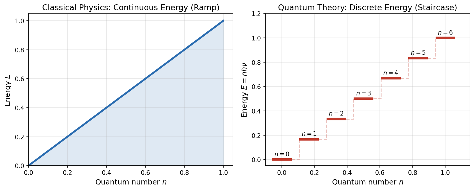
Fig. 0.1: Continuous vs. discrete energy. In classical physics, energy changes continuously (left, ramp). In quantum theory, energy can only take discrete values (right, staircase). The oscillator energy that Planck introduced to explain blackbody radiation was an integer multiple of \(h\nu\) (\(h\): Planck's constant, \(\nu\): frequency), but the spacing between energy levels of a general atom is not necessarily uniform.

2. Chemical Bonds — Why Do Atoms Stick Together?

🟡 Lina: A water molecule H₂O is made of 2 hydrogen atoms and 1 oxygen atom stuck together. But if you try to explain "why they stick" using Newtonian mechanics, it doesn't work.

⚪ Mei: Isn't it electrical attraction? Positive and negative charges attracting each other?

🟡 Lina: That alone is insufficient. To answer questions like which direction atoms bond in, at what distance they bond, why hydrogen forms a stable molecule H₂ with two atoms while helium doesn't form He₂—you need to calculate the overlap of electron wave functions. A wave function is, roughly speaking, "a mathematical function that tells you where an electron is likely to be found and with what probability." However, there's a bit more precision needed in this "roughly speaking" part, and I'll correct it later. The formal definition comes in Ch. 7, so for now let's proceed with this rough understanding. Chemistry is fundamentally built on quantum mechanics.

🔵 Kai: Even chemistry is quantum mechanics! But in high school chemistry, we learned that "a covalent bond shares electrons"—isn't that enough?

🟡 Lina: The phrase "sharing electrons" is correct, but to understand why sharing makes things stable, or why bonds form in specific directions, you need to calculate the electron wave functions. The physicist Dirac wrote in 1929: "The underlying physical laws necessary for the mathematical theory of a large part of physics and the whole of chemistry are thus completely known." Of course, actually performing the calculations is enormously difficult, but the fundamental principles are given by quantum mechanics.

🔵 Kai: "Completely known"—that's quite confident... Is it really true?

🟡 Lina: In principle, yes. But "known in principle" and "actually computable" are different problems. For example, proteins consist of thousands of atoms, and predicting their folding directly from quantum mechanical equations is still beyond current supercomputers because there are too many electrons involved. But the fundamental laws themselves are given by quantum mechanics—that was Dirac's claim.

3. Semiconductors and Transistors — The Foundation of Modern Civilization

🟡 Lina: The semiconductor chip in the smartphone I mentioned earlier. By mixing tiny amounts of impurities into crystals of the element silicon, you can precisely control the flow of electricity. The question "why does mixing impurities change electrical properties" is explained by quantum mechanics' band theory.

⚪ Mei: Transistors too?

🟡 Lina: Transistors were invented at Bell Laboratories in 1947, and their operating principle is pure quantum mechanics. Today, a single chip contains tens of billions of transistors. Without quantum mechanics, neither modern computers nor the internet would exist.

4. Lasers — Aligning Light

🟡 Lina: Do you know why the light from a laser pointer is so straight and uniform in color?

🔵 Kai: What makes it different from ordinary light?

🟡 Lina: Ordinary light—like light from a light bulb—consists of various frequencies emitted in random directions at random timings. In a laser, all photons come out with the same frequency, same direction, and same timing (phase). "Phase" refers to the timing of a wave's peaks and troughs, and I'll explain this in more detail shortly. The key mechanism for "aligning" them is stimulated emission, a quantum mechanical phenomenon predicted by Einstein in 1917.

⚪ Mei: Einstein predicted the principle behind lasers.

🟡 Lina: Yes. The laser was actually built in 1960, so it took over 40 years from prediction to realization. In Ch. 21, we'll learn the quantitative treatment of stimulated emission—Einstein's A and B coefficients.

5. Superconductivity and Superfluidity — A World of Zero Resistance

🟡 Lina: When certain materials are cooled to extremely low temperatures, their electrical resistance drops completely to zero. This is superconductivity. It's used in the powerful magnets of MRI (magnetic resonance imaging) machines and in magnetic levitation trains. This phenomenon, too, cannot be understood without quantum mechanics.

🔵 Kai: Zero electrical resistance! Does that mean free electricity...?

🟡 Lina: It takes energy to cool things down, so it's not that simple. But superconductivity is a dramatic example where quantum mechanical effects manifest at macroscopic scales. Roughly speaking, electrons form pairs and collectively "condense" into a single quantum state, becoming immune to scattering. The details will become clearer after we learn the statistics of identical particles in Ch. 18.

6. Quantum Entanglement and Quantum Computing — The 21st Century Frontier

🟡 Lina: And finally, a field where cutting-edge research is actively underway right now. Quantum entanglement and quantum computation.

🔵 Kai: I hear about quantum computers in the news a lot.

🟡 Lina: Quantum entanglement is a correlation that cannot be explained by classical physics—when two particles are separated, measuring one instantly determines the state of the other. Einstein called this "spooky action at a distance" and hated it. But experiments have shown that this "spooky correlation" is real. We'll cover this in detail in Ch. 23 and Ch. 24.

🔵 Kai: But if measuring one instantly determines the other, can't you send information faster than light? Doesn't that contradict relativity?

🟡 Lina: Sharp question. The short answer is: quantum entanglement does not transmit information faster than light. "There's correlation but no communication"—we'll verify this subtle distinction quantitatively in Ch. 24. In any case, this is not science fiction but experimentally verified fact. And quantum computers use this quantum entanglement as a computational resource. Calculations that would take conventional computers tens of thousands of years could potentially be done by quantum computers in a short time.

---

🟡 Lina: To summarize what we've covered so far, here's an overview of the phenomena and technologies involving quantum mechanics. See Table 0.1 "Overview of phenomena and technologies involving quantum mechanics and their coverage in this book".

Table 0.1: Overview of phenomena and technologies involving quantum mechanics and their coverage in this book

Phenomenon/Technology	Quantum Mechanical Involvement	Coverage in This Book
Atomic spectra	Discreteness of energy	Ch. 1, Ch. 16
Chemical bonds	Overlap of wave functions	Ch. 7 (introduction of wave functions), Ch. 18 (Pauli principle and electron configuration as foundation)
Semiconductors/Transistors	Band theory	Ch. 9 (fundamentals)
Lasers	Stimulated emission	Ch. 6 (maser), Ch. 21 (A & B coefficients)
Superconductivity/Superfluidity	Macroscopic quantum effects	Ch. 18 (statistics of identical particles as foundation)
MRI	Nuclear spin resonance	Ch. 6, Ch. 17
Quantum entanglement	Non-local correlations	Ch. 23, Ch. 24
Quantum computers	Superposition & entanglement	Ch. 24

🔵 Kai: It covers that much...? From a single atom to computers.

🟡 Lina: That's why quantum mechanics is called "the most successful model of the 20th century." For over 100 years, within its domain of applicability—that is, situations where gravity can be ignored—there hasn't been a single case where its predictions disagreed with experiment. It continues to describe nature with astonishing precision.

⚪ Mei: But it's still a "hypothesis," right?

🟡 Lina: Yes. No matter how successful, it remains a hypothesis. If it's falsified by experiment, it will be replaced by a better model. In fact, quantum mechanics and general relativity—the model of gravity—contradict each other, and under extreme conditions (like the center of a black hole or the beginning of the universe), both cannot be applied simultaneously. A model of "quantum gravity" that unifies both has not yet been found. We'll discuss this in Ch. 28.

✅ Comprehension Check: Briefly explain, from the quantum mechanical perspective, why atomic spectra show "only specific colors."

Answer

Because the energies that electrons in atoms can have are discrete, the energy of light emitted when electrons transition between energy levels is also discrete. Discrete energies mean discrete frequencies (colors), and as a result, only specific colors of light are emitted.

✅ Comprehension Check: Name three technologies involving quantum mechanics and briefly state what property of quantum mechanics is relevant to each.

Answer

Examples: (1) Semiconductors (wave-like nature of electrons and band structure), (2) Lasers (stimulated emission—a quantum mechanical process where photons align into the same state), (3) MRI (quantum mechanical resonance of nuclear spins). Other examples include atomic spectra (discreteness of energy), quantum computers (superposition and quantum entanglement), etc.

---

The Core of Quantum Mechanics — The World Is Made of Complex Probability Amplitudes

🟡 Lina: Now, you've seen how wide a range of phenomena quantum mechanics covers. So what is its core? In one sentence:

The world is made of superpositions of complex probability amplitudes.

🔵 Kai: ...I don't understand at all. "Complex" and "amplitude" don't click for me.

🟡 Lina: That's fine—this is just a "taste" for now. "Complex numbers" are numbers using \(i = \sqrt{-1}\) that you learned in high school, and "amplitude" is something like the height of a wave—except "probability amplitude" isn't a physical wave height but a mathematical quantity for calculating probabilities. You'll come to understand the precise meaning one by one during the journey. But it's important to check the destination on the map before setting out, right?

🔵 Kai: I see, so we're just looking at the destination for now. Got it.

🟡 Lina: First, recall the world of high school physics. When you throw a ball, its position is determined by a function of time \(x(t)\). If you know the initial conditions—the position and velocity when thrown—you can completely predict the future trajectory. This is the classical mechanics worldview—a deterministic worldview.

⚪ Mei: So if the initial conditions are determined, the future is uniquely determined.

🟡 Lina: Exactly. But at the atomic scale, this worldview breaks down fundamentally. Where an electron is located is "not determined" until measured. What is determined is only the probability of finding the electron at each position when measured.

🔵 Kai: Probability... Like dice?

🟡 Lina: There's a crucial difference from dice. With dice, the probability of each face is \(1/6\), and you add probabilities to get the total probability. But in quantum mechanics, instead of adding probabilities directly, you add probability amplitudes—which are complex numbers—and then take the absolute value squared to get the probability.

🟡 Lina: The physicist Feynman described this most vividly. He compared experiments with bullets, waves, and electrons. We'll cover the double-slit experiment in detail in Ch. 3, but here's just the essence.

---

The Case of Bullets — Addition of Probabilities

🟡 Lina: Imagine an experiment where bullets are fired from a machine gun at a screen behind a wall with two holes. Let \(P_1(x)\) be the probability that a bullet reaches position \(x\) on the screen when only hole 1 is open, and \(P_2(x)\) when only hole 2 is open.

🔵 Kai: Does the \(x\) in \(P_1(x)\) mean the location on the screen?

🟡 Lina: Yes. Strictly speaking, it should be called "probability density"—meaning "the probability of arriving within a narrow width \(\Delta x\) near position \(x\) is approximately \(P(x) \times \Delta x\)." But for now, just think of it as "how likely it is to arrive at position \(x\)." The formal definition comes in Ch. 7.

🔵 Kai: Is "probability density" different from "probability"?

🟡 Lina: For continuous quantities (like position), there are infinitely many possible values, so the probability of hitting any single exact value is zero—it's the same feeling as the probability of a dart hitting "this mathematically exact point" being zero. The area of the target is finite, but the area of a point is zero, so the probability of hitting a single point is also zero. But there's a finite probability of hitting a small region "around here"—say, within 1 cm radius of the center. So we consider "the probability of arriving in a small interval of width \(\Delta x\)" and divide by \(\Delta x\) to get the probability density. No need to go deep into this now—just think of it as "the concentration of likelihood." OK?

🔵 Kai: Hmm, "the probability of a single point being zero" is a bit strange... but "probability density is the probability of arriving in a narrow width divided by that width"—I'll go with that for now. OK, back to the main topic—if both holes are open, the bullet must pass through one or the other, so shouldn't we just add both probabilities?

🟡 Lina: Exactly right. Since a bullet necessarily passes through one hole or the other,

\[ P_{12} = P_1 + P_2 \]

This is how classical particles behave. It matches intuition. Look at Fig. 0.2 "Conceptual diagram of the bullet double-slit experiment. (a) Bullets fired from machine gun S pass through holes 1 and 2 and hit the screen. (b) Probability distributions \(P_1\), \(P_2\) when each hole alone is open. (c) Probability distribution with both open: \(P_{12} = P_1 + P_2\)"—it shows bullets from machine gun S passing through holes 1 and 2 in the wall and hitting the screen.

🔵 Kai: Looking at the figure, \(P_{12} = P_1 + P_2\) makes sense. But this holds because of the assumption that "the bullet necessarily passes through one or the other," right? If a bullet could pass through both holes simultaneously, would things be different?

🟡 Lina: That's exactly the question that matters in the "electron case" coming up. The assumption breaks down for electrons—remember that. Looking at Fig. 0.2 "Conceptual diagram of the bullet double-slit experiment. (a) Bullets fired from machine gun S pass through holes 1 and 2 and hit the screen. (b) Probability distributions \(P_1\), \(P_2\) when each hole alone is open. (c) Probability distribution with both open: \(P_{12} = P_1 + P_2\)" (c), you can see that on the screen, the peaks corresponding to the two holes simply overlap, with no interference fringes appearing.

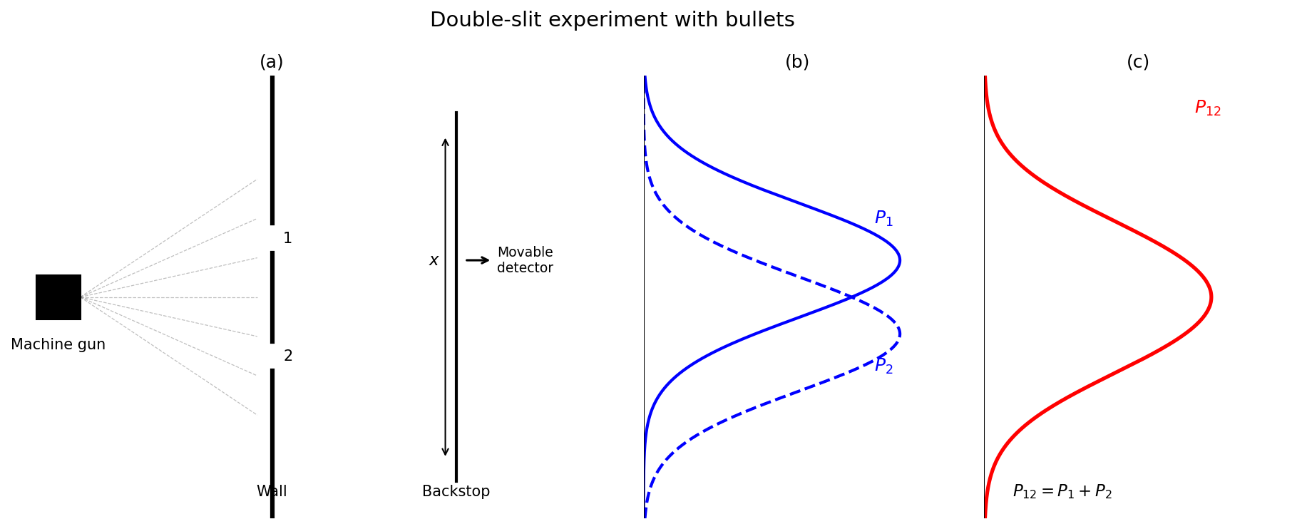
Fig. 0.2: Conceptual diagram of the bullet double-slit experiment. (a) Bullets fired from machine gun S pass through holes 1 and 2 and hit the screen. (b) Probability distributions \(P_1\), \(P_2\) when each hole alone is open. (c) Probability distribution with both open: \(P_{12} = P_1 + P_2\)—no interference.

The Case of Waves — Interference

🟡 Lina: Now consider water waves. Waves from a source pass through two holes and reach a screen. The intensity of a wave (a quantity proportional to energy) is proportional to the square of the amplitude—the height of the wave. Why the square? Because the energy of a wave is determined by the square of the oscillation's magnitude. For example, the elastic energy of a spring you learned in high school, \(\frac{1}{2}kx^2\), is proportional to the square of displacement \(x\), right? Waves work the same way—each point on the water surface oscillates like a spring, so the larger the oscillation, the greater the energy—and the relationship is proportional to the square. The same goes for sound waves: the loudness (intensity) of sound is proportional to the square of the air vibration's amplitude. For now, just accept the rule "intensity ∝ amplitude²." To describe waves, we need not only amplitude (size) but also another important quantity: phase.

🔵 Kai: Phase? Like the "shift" of a wave?

🟡 Lina: That's exactly the right image. Let me explain a bit more precisely. Even two waves with the same frequency can have their peaks and troughs shifted in timing.

🔵 Kai: By "shift," do you mean something like one wave arriving slightly later?

🟡 Lina: Yes, exactly that image. Since waves are repetitive motion, we express "what stage of oscillation it's currently at" as an angle—that's called the phase. For example, with a pendulum: when it's at the right end, that's 0°; passing through the middle going left is 90°; at the left end is 180°; passing through the middle going right is 270°—and when it returns to the right end, it's 360° = 0° again. One period corresponds to one full cycle (\(2\pi\) radians = 360°). The difference in phase between two waves—"how much they're shifted"—is called the phase difference. For example, if they're shifted by half a period, the phase difference is \(\pi\) (180°); if not shifted at all, it's \(0\). If the phase difference is \(0\), peaks align with peaks; if it's \(\pi\), peaks align with troughs.

🔵 Kai: I understand mapping one period to 360°, but why use radians instead of degrees?

🟡 Lina: When using \(\cos\) and \(\sin\) in equations, measuring in radians keeps formulas simple. For example, the derivative of \(\sin\theta\) is \(\cos\theta\)—this only holds when using radians. The \(\theta\) in \(e^{i\theta}\) that appears later is also in radians. In physics, angles are almost always written in radians.

⚪ Mei: Phase difference of \(0\) means constructive interference, \(\pi\) means destructive—I understand that. But when actually adding two waves, how do you handle amplitude and phase?

🟡 Lina: Good question. When adding two waves, you need to consider not only each wave's amplitude (height) but also its phase (timing shift). For example, the wave arriving at position \(x\) on the screen from hole 1 can be written as a sinusoidal wave \(a_1 \cos(\omega t + \theta_1)\)—\(a_1\) is the amplitude, \(\theta_1\) is the phase, and \(\omega\) (omega) is the angular frequency representing the rate of oscillation. If you try to add two sinusoidal waves and find the intensity, you end up expanding addition formulas—like \(\cos(\alpha + \beta) = \cos\alpha\cos\beta - \sin\alpha\sin\beta\)—and the terms keep multiplying, making it messy.

🔵 Kai: Yeah, I remember trigonometric addition formulas being tedious... Is there an easier way?

🟡 Lina: There is. You package the amplitude and phase into a single complex number. Specifically, you represent the wave \(a\cos(\omega t + \theta)\) by the complex number \(ae^{i\theta}\)—a complex number with magnitude \(a\) and angle \(\theta\). You might wonder "where did the \(\omega t\) part go?"—but when adding waves of the same frequency, the \(\omega t\) part is common to all of them, so only the phase difference \(\theta\) matters in the comparison. That's why we can omit \(\omega t\) and compare just \(ae^{i\theta}\). This way, adding waves becomes adding complex numbers, and calculating intensity is just "taking the absolute value squared." The notation \(e^{i\theta}\) means "a complex number with magnitude 1 and angle \(\theta\)."

Let me explain the complex plane here. It's a plane with the real part on the horizontal axis (the ordinary number line) and the imaginary part on the vertical axis (multiples of \(i\)). For example, \(1 + i\) is the point at horizontal 1, vertical 1; \(2i\) is at horizontal 0, vertical 2. On this plane, \(e^{i\theta}\) moves along a circle of radius 1 centered at the origin—it's the point at angle \(\theta\) counterclockwise from the real axis (horizontal axis). This comes from Euler's formula \(e^{i\theta} = \cos\theta + i\sin\theta\)—since \(\cos\theta\) is the real part (horizontal coordinate) and \(\sin\theta\) is the imaginary part (vertical coordinate), the distance from the origin is \(\sqrt{\cos^2\theta + \sin^2\theta} = 1\), confirming it lies on the unit circle. I've drawn this in Fig. 0.3 "The complex plane and \(e^{i\theta}\)", so check it out.

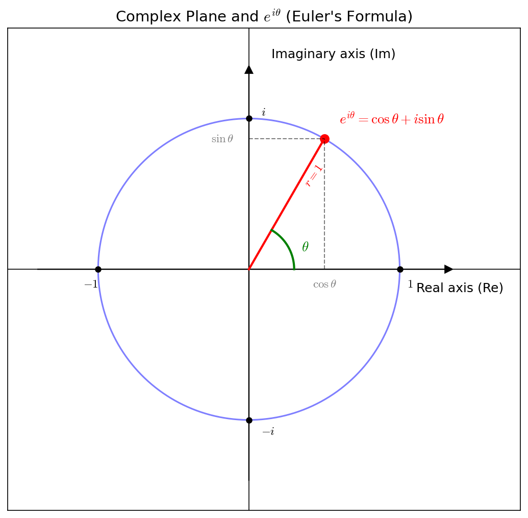
Fig. 0.3: The complex plane and \(e^{i\theta}\). The horizontal axis is the real part, the vertical axis is the imaginary part. \(e^{i\theta}\) is a point on the unit circle (radius 1 circle centered at the origin), at angle \(\theta\) counterclockwise from the real axis.

🔵 Kai: Wait a moment. \(e\) is the 2.718... \(e\), right? Why does an exponential function connect to \(\cos\) and \(\sin\)?

🟡 Lina: A very good question. To derive it properly requires Taylor expansion (a method of representing functions as infinite series). It's done carefully in Appendix A, so check there if you're curious. At this stage, you can think of \(e^{i\theta}\) as simply a definition—"a notation representing the point at distance 1 from the origin and angle \(\theta\) on the complex plane." In fact, the convenience of this notation lies in the fact that "multiplication becomes addition of angles" (\(e^{i\alpha} \cdot e^{i\beta} = e^{i(\alpha+\beta)}\)), which we'll use right away so you'll feel its power. Just take home the rule: "amplitude \(a\) and phase \(\theta\) are written together as \(ae^{i\theta}\)." As we confirmed on the complex plane, \(e^{i\theta}\) was a point on the unit circle—magnitude 1, angle \(\theta\). When you multiply it by a positive real number \(a\), the magnitude stretches by a factor of \(a\), giving the point "magnitude \(a\), angle \(\theta\)." In other words, \(ae^{i\theta}\) is a single complex number on the complex plane representing "distance from origin = \(a\) (= wave magnitude), angle = \(\theta\) (= phase)." This "complex number that packages amplitude and phase, \(ae^{i\theta}\)," is called the complex amplitude. Write the complex amplitude of the wave from hole 1 as \(h_1 = a_1 e^{i\theta_1}\) and from hole 2 as \(h_2 = a_2 e^{i\theta_2}\) (\(a_1, a_2\) are positive real numbers representing wave magnitudes, \(\theta_1, \theta_2\) are phases). The intensity of a single wave is given by the absolute value squared of its complex amplitude—for example, if only hole 1 is open, the intensity is \(|h_1|^2\); if only hole 2, it's \(|h_2|^2\). The "magnitude (absolute value)" of a complex number means, for \(z = a + bi\), \(|z| = \sqrt{a^2 + b^2}\)—the distance from the origin on the complex plane. Therefore \(|ae^{i\theta}|^2 = a^2 \cdot |e^{i\theta}|^2 = a^2 \cdot 1 = a^2\), which is consistent with what I said about "proportional to amplitude squared." When both holes are open, the complex amplitudes superpose, so the intensity is

\[ I_{12} = |h_1 + h_2|^2 \]

🟡 Lina: Now, do you think this simply equals \(|h_1|^2 + |h_2|^2\)?

🔵 Kai: Wait, it doesn't? Just adding the intensity of wave 1 and wave 2...

🟡 Lina: Even with real numbers, \((a+b)^2\) doesn't equal \(a^2 + b^2\), right? An extra \(2ab\) term appears. The same thing happens with complex numbers.

🔵 Kai: Ah, right... \((a+b)^2 = a^2 + 2ab + b^2\), so with complex numbers an extra term appears too.

🟡 Lina: Exactly. When expanded, the final result is this—I'll just show you the conclusion for now. The derivation comes right after, so you don't need to memorize it.

\[ |h_1 + h_2|^2 = |h_1|^2 + |h_2|^2 + 2|h_1||h_2|\cos\delta \]

Here \(\delta = \theta_1 - \theta_2\) is the phase difference between the two waves.

🔵 Kai: Hold on. I see the result, but where does the \(\cos\delta\) come from? It seems to appear out of nowhere...

🟡 Lina: That's a fair concern. Let me first show you the conclusion. For example, when \(h_1 = 1\) and \(h_2 = e^{i\pi/3}\), calculating \(|h_1 + h_2|^2\) gives \(3\)—it's not simply \(|h_1|^2 + |h_2|^2 = 1 + 1 = 2\). The difference between "\(2\) vs. \(3\)" is the interference term. Now, why does it equal \(3\)? I said earlier that "intensity is the absolute value squared of the complex amplitude \(|h|^2\)." To actually calculate \(|h_1 + h_2|^2\), we need "a mechanical method for finding the absolute value squared of a complex number." The tool for this is the complex conjugate. The procedure is simple—for a complex number \(z = a + bi\), flip the sign of the imaginary part to get \(\bar{z} = a - bi\), called the complex conjugate. For example, if \(z = 3 + 2i\) then \(\bar{z} = 3 - 2i\).

🔵 Kai: You just flip the \(+\) to \(-\) in the imaginary part? But what's useful about multiplying them together?

🟡 Lina: Try multiplying these two: \(z\bar{z} = (a + bi)(a - bi) = a^2 - (bi)^2 = a^2 + b^2\)—since \(i^2 = -1\), the minus sign cancels. So \(|z|^2 = z\bar{z} = a^2 + b^2\). The rule is: "the squared magnitude of a complex number is obtained by multiplying it by its complex conjugate."

⚪ Mei: Ah, \((a + bi)(a - bi)\) is the same form as \((a+b)(a-b) = a^2 - b^2\) from high school. With \(bi\) instead of \(b\), the \(-b^2\) becomes \(+b^2\).

🟡 Lina: Perfect. The formula \(|z|^2 = z\bar{z}\) holds for any complex number \(z\). So you can substitute \(h_1 + h_2\) as a whole in place of \(z\). A lot of new tools have appeared all at once, but you don't need to memorize everything right now. The important thing is just the conclusion: "adding first and then squaring produces an extra term." You'll use complex number calculations repeatedly from Ch. 4 onward, so they'll become natural.

🔵 Kai: Wait, isn't \(z\) supposed to be a single complex number? \(h_1 + h_2\) is the sum of two complex numbers...

🟡 Lina: Good question. \(h_1 + h_2\), once added, is still a single complex number, right? For example, if \(h_1 = 1+i\) and \(h_2 = 2+3i\), then \(h_1 + h_2 = 3+4i\)—a single complex number. So \(|z|^2 = z\bar{z}\) holds no matter what you put in for \(z\). One supplement here—the complex conjugate of a sum equals the sum of the complex conjugates. That is, \(\overline{h_1 + h_2} = \bar{h}_1 + \bar{h}_2\). Check: the complex conjugate of \(h_1 + h_2 = 3 + 4i\) is \(3 - 4i\). Meanwhile, \(\bar{h}_1 + \bar{h}_2 = (1-i) + (2-3i) = 3 - 4i\). They match. Therefore \(|h_1 + h_2|^2 = (h_1 + h_2)(\bar{h}_1 + \bar{h}_2)\) can be expanded, and besides \(|h_1|^2 + |h_2|^2\), "cross terms" \(h_1 \bar{h}_2 + \bar{h}_1 h_2\) appear.

🔵 Kai: Cross terms... The "extra terms" that come out when you expand.

🟡 Lina: Right. Now, since \(h_1 = a_1 e^{i\theta_1}\) and \(h_2 = a_2 e^{i\theta_2}\), the complex conjugate of \(h_2\) is \(\bar{h}_2 = a_2 e^{-i\theta_2}\). Why? Because by Euler's formula, \(e^{i\theta_2} = \cos\theta_2 + i\sin\theta_2\), and flipping the sign of the imaginary part gives \(\cos\theta_2 - i\sin\theta_2 = e^{-i\theta_2}\).

🔵 Kai: So taking the complex conjugate flips the sign in front of \(i\) in the exponent.

🟡 Lina: Exactly. The complex conjugate of \(e^{i\theta}\) is \(e^{-i\theta}\)—that's handy to remember. Now, calculating \(h_1 \bar{h}_2\), using the exponent rule \(e^a \cdot e^b = e^{a+b}\): \(h_1 \bar{h}_2 = a_1 a_2 e^{i\theta_1} e^{-i\theta_2} = a_1 a_2 e^{i(\theta_1 - \theta_2)} = a_1 a_2 e^{i\delta}\). Similarly, \(\bar{h}_1 h_2 = a_1 a_2 e^{-i\delta}\).

🔵 Kai: Let me check—\(e^{i\theta_1} \cdot e^{-i\theta_2}\) means adding the exponents to get \(i(\theta_1 - \theta_2) = i\delta\), right? So we get two terms, \(e^{i\delta}\) and \(e^{-i\delta}\). What happens when you add them?

🟡 Lina: Expand \(e^{i\delta} + e^{-i\delta}\) using Euler's formula. \(e^{i\delta} = \cos\delta + i\sin\delta\), \(e^{-i\delta} = \cos\delta - i\sin\delta\). When you add them?

⚪ Mei: The \(i\sin\delta\) and \(-i\sin\delta\) cancel, leaving only \(2\cos\delta\).

🟡 Lina: Perfect. So the cross terms become \(a_1 a_2 \times 2\cos\delta = 2|h_1||h_2|\cos\delta\). You can see how the phase difference \(\delta\) determines the result. Since \(\delta\) varies at different locations on the screen, at some places \(\cos\delta > 0\) giving constructive interference, and at other places \(\cos\delta < 0\) giving destructive interference—this is how the pattern of bright and dark fringes (interference pattern) appears. Compared to Fig. 0.2 "Conceptual diagram of the bullet double-slit experiment. (a) Bullets fired from machine gun S pass through holes 1 and 2 and hit the screen. (b) Probability distributions \(P_1\), \(P_2\) when each hole alone is open. (c) Probability distribution with both open: \(P_{12} = P_1 + P_2\)" (c) for bullets, the crucial difference with waves is that instead of simple overlapping peaks, you get a fringe pattern. This interference pattern has essentially the same form as what we'll see for electrons in Fig. 0.4 "Conceptual diagram of the electron double-slit experiment. (a) Electrons fired from electron gun S are detected one at a time with a "click." (b) Probability distributions \(P_1\), \(P_2\) when each hole alone is open. (c) Probability distribution with both open: \(P_{12}\)" (c). (The interference pattern for water waves has the same form as the electron figure Fig. 0.4 "Conceptual diagram of the electron double-slit experiment. (a) Electrons fired from electron gun S are detected one at a time with a "click." (b) Probability distributions \(P_1\), \(P_2\) when each hole alone is open. (c) Probability distribution with both open: \(P_{12}\)" (c), so check it there.) Let's verify with a concrete example. If \(h_1 = e^{i \cdot 0} = 1\) and \(h_2 = e^{i\pi/3}\), the phase difference is \(\delta = 0 - \pi/3 = -\pi/3\). Since \(\cos\) is an even function, \(\cos(-\pi/3) = \cos(\pi/3) = 1/2\). Applying the formula: \(|1 + e^{i\pi/3}|^2 = 1 + 1 + 2\cos(\pi/3) = 2 + 2 \times \frac{1}{2} = 3\)—it doesn't simply equal \(|h_1|^2 + |h_2|^2 = 1 + 1 = 2\), does it?

🔵 Kai: Honestly, the part where \(\cos\) emerges from the cross terms is still a bit fuzzy for me... Specifically, I understand that adding \(e^{i\delta}\) and \(e^{-i\delta}\) gives \(\cos\) as a calculation, but I don't intuitively feel "why \(\cos\)?" But I do understand that "adding first and then squaring produces an extra term." Simply adding gives \(1 + 1 = 2\), but because of the interference term it becomes \(3\)—seeing it with concrete numbers, there's definitely a difference.

🟡 Lina: That fuzziness is healthy. To restate in one sentence why \(\cos\) appears: "Adding \(e^{i\delta}\) and \(e^{-i\delta}\) cancels the imaginary parts, leaving only the real part—which is \(2\cos\delta\)." On the complex plane, the points at angles \(+\delta\) and \(-\delta\) are mirror images about the real axis, so when you add them, the imaginary parts cancel—geometrically natural, right? In other words, \(\cos\) appearing is a reflection of the geometric fact that "adding mirror-image points gives a point on the real axis." But what I want you to remember today isn't the detailed mechanism—just the conclusion. "When you add two waves and then square, an extra term (interference term) appears depending on the phase difference \(\delta\)"—that's today's message. Complex conjugates and Euler's formula are just tools for deriving that conclusion, so you don't need to memorize them all right now. Let me show one more concrete example: if \(h_1 = 1\) and \(h_2 = e^{i\pi} = -1\), then \(|1 + (-1)|^2 = 0\)—complete cancellation. Applying the formula: \(1 + 1 + 2\cos\pi = 2 - 2 = 0\), which matches.

🔵 Kai: Wow, with phase difference \(\pi\) it's completely zero! They cancel perfectly.

🟡 Lina: Phase difference \(0\) means constructive interference, \(\pi\) means complete cancellation—\(\cos\) represents the degree of "constructive ↔ destructive." To summarize: thanks to the interference term \(2|h_1||h_2|\cos\delta\), waves strengthen at some places and weaken at others. So \(I_{12} \neq I_1 + I_2\). That's interference.

The Case of Electrons — Particles That Interfere

🟡 Lina: Now, finally, electrons. Earlier when discussing chemical bonds, I said "the wave function is a function that determines the probability of where an electron will be found." That's not wrong, but let me state it more precisely. A wave function is a function that assigns a probability amplitude (a complex number) to each position \(x\). It doesn't directly give the probability—first it gives the probability amplitude, and then the absolute value squared \(|\psi(x)|^2\) becomes "the probability of finding the electron at position \(x\)." So "determines the probability" meant "determines the probability via the probability amplitude"—I've just refined the earlier explanation by one level.

🔵 Kai: Ah, it's the same structure as the water wave where "amplitude squared equals intensity." The wave function is the amplitude, and its square is the probability.

🟡 Lina: Exactly that correspondence. Leaving the precise definition to Ch. 7, let's focus on probability amplitudes now. Fire electrons one at a time from an electron gun. When one reaches the screen, it goes "click"—detected one at a time, as particles. So far, same as bullets.

🔵 Kai: If they arrive one at a time as particles, shouldn't we just add probabilities like bullets...?

🟡 Lina: But when you fire many electrons and examine the probability distribution,

\[ P_{12} \neq P_1 + P_2 \]

Different from the bullet result. And amazingly, the distribution pattern of \(P_{12}\) looks exactly like the interference pattern of water waves.

🔵 Kai: What? They arrive one at a time as particles, but the overall pattern shows wave interference?

🟡 Lina: Look at Fig. 0.4 "Conceptual diagram of the electron double-slit experiment. (a) Electrons fired from electron gun S are detected one at a time with a "click." (b) Probability distributions \(P_1\), \(P_2\) when each hole alone is open. (c) Probability distribution with both open: \(P_{12}\)". Individual electrons arrive with a "click" at single points, yet when many accumulate, the fringe pattern of (c) emerges. Compare with Fig. 0.2 "Conceptual diagram of the bullet double-slit experiment. (a) Bullets fired from machine gun S pass through holes 1 and 2 and hit the screen. (b) Probability distributions \(P_1\), \(P_2\) when each hole alone is open. (c) Probability distribution with both open: \(P_{12} = P_1 + P_2\)" (c)—for bullets, the peaks simply overlapped, but for electrons, bright and dark fringes appear. Completely different patterns, right?

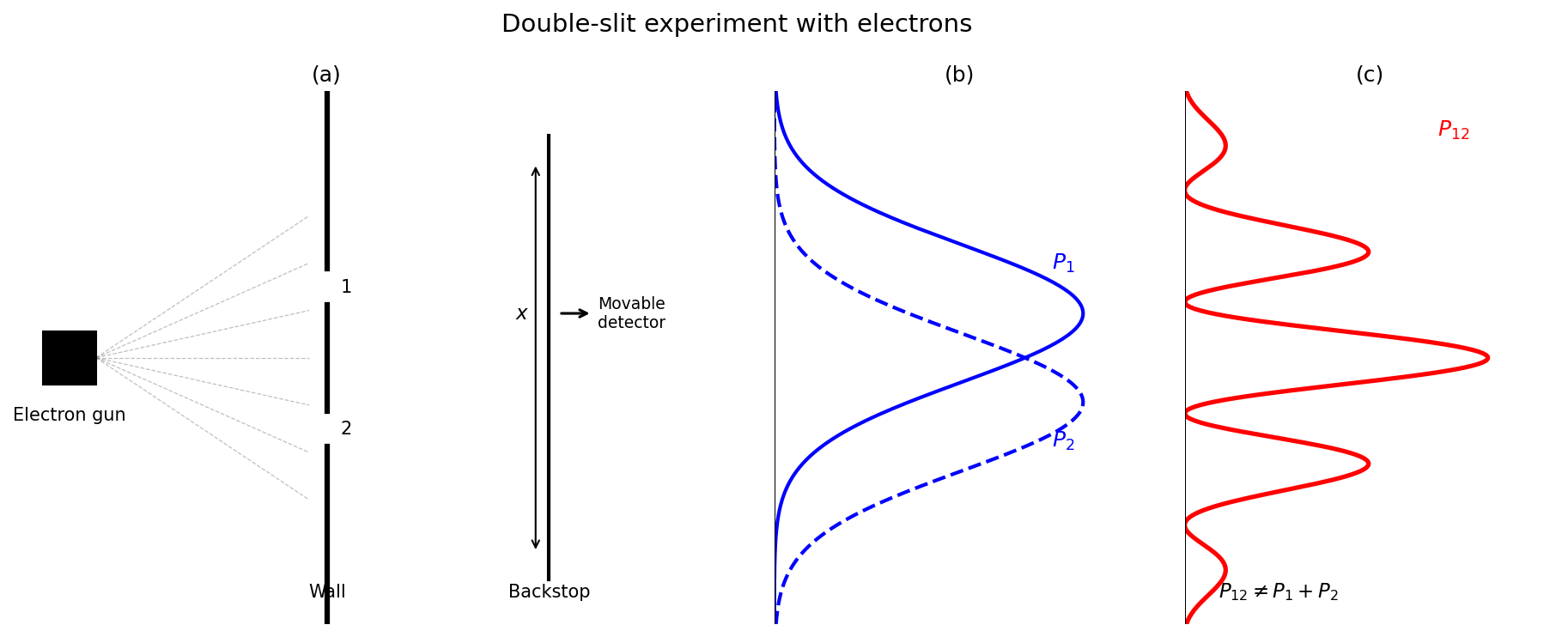
Fig. 0.4: Conceptual diagram of the electron double-slit experiment. (a) Electrons fired from electron gun S are detected one at a time with a "click." (b) Probability distributions \(P_1\), \(P_2\) when each hole alone is open. (c) Probability distribution with both open: \(P_{12}\)—unlike bullets, an interference pattern appears (\(P_{12} \neq P_1 + P_2\)).

🟡 Lina: Yes. This is the core of quantum mechanics. Mathematically, it's written as follows. Let \(\phi_1(x)\) be the probability amplitude for the electron to pass through hole 1 and arrive at position \(x\), and \(\phi_2(x)\) be the probability amplitude for passing through hole 2—here \(\phi\) (phi) is a symbol representing "the probability amplitude for each path." For water waves we wrote the complex amplitude as \(h\), but for electrons it's not a physical wave but "a mathematical quantity for calculating probabilities," so we use a different symbol \(\phi\) to distinguish them. Probability amplitudes are complex numbers, and their absolute value squared gives the probability:

\[ P_1 = |\phi_1|^2, \quad P_2 = |\phi_2|^2, \quad P_{12} = |\phi_1 + \phi_2|^2 \]

Exactly the same structure as the water wave complex amplitude formula.

⚪ Mei: So both water waves and electrons mathematically perform the same operation—"add complex numbers, then take the absolute value squared."

🟡 Lina: Exactly. Instead of adding probabilities directly, you add probability amplitudes and then square. That's why interference occurs.

⚪ Mei: Bullets use "addition of probabilities," electrons use "addition of amplitudes → squaring." That difference determines whether interference occurs or not.

🔵 Kai: Wait. Electrons arrive one at a time with a "click," right? Does that mean a single electron passes through both holes simultaneously?

🟡 Lina: That question strikes at the heart of the matter. If you try to determine "which hole the electron passed through," the interference pattern disappears. We'll cover this in detail in Ch. 3, so for now just take home the rule "add the probability amplitudes." And these probability amplitudes must be complex numbers. Real numbers alone cannot reproduce quantum mechanics' predictions.

🔵 Kai: Why complex numbers? What's wrong with real numbers?

🟡 Lina: A very good question. For now I'll just say "experiments demand it." In Ch. 4 you'll learn Feynman's probability amplitude rules, and from Ch. 5 onward, when you calculate concrete two-state systems, you'll come to feel that complex numbers are indispensable.

🔵 Kai: I see... Honestly I'm still a bit fuzzy. Just one thing—with water waves, \(\cos\) appeared and we got interference, right? That should be doable with real number calculations alone. So why do electrons "require complex numbers"—what's different?

🟡 Lina: That's a question that strikes at the core. For water waves, the amplitude can indeed be described with real numbers. But the probability amplitude for electrons has a structure where the phase rotates continuously in time like \(e^{i\omega t}\), which cannot be expressed with real numbers. Exactly what differs will become clear when you learn Feynman's rules in Ch. 4. Hold onto that "fuzziness." Now, the axis of this journey is:

The world is made of superpositions of complex probability amplitudes.

— Pursue this with equations, and judge for yourself. That's the axis of this journey.

Complex numbers called probability amplitudes are the starting point for all predictions of quantum mechanics. In this journey, we'll trace these equations step by step, verifying "why can we write it this way," "what does it predict," and "does it agree with experiments" with your own eyes.

✅ Comprehension Check: In the water wave interference formula \(|h_1 + h_2|^2 = |h_1|^2 + |h_2|^2 + 2|h_1||h_2|\cos\delta\), what effect does the interference term \(2|h_1||h_2|\cos\delta\) produce?

Answer

Depending on the value of the phase difference \(\delta\), waves constructively interfere (\(\cos\delta > 0\)) or destructively interfere (\(\cos\delta < 0\)). This causes the intensity to vary across different locations on the screen, producing a pattern of bright and dark fringes (interference pattern).

✅ Comprehension Check: In the bullet double-slit experiment, \(P_{12} = P_1 + P_2\) holds, but for electrons it does not. State in one sentence the mathematical mechanism that produces this difference.

Answer

For electrons, instead of adding probabilities directly, probability amplitudes (complex numbers) are added first and then the absolute value squared is taken, so an interference term appears and \(P_{12} \neq P_1 + P_2\).

---

Einstein and Quantum Mechanics — Founder and Greatest Critic

🟡 Lina: Now I'd like to tell you about a figure who will appear repeatedly throughout this journey. Albert Einstein.

🔵 Kai: Einstein is the relativity guy, right? \(E = mc^2\) and all that.

🟡 Lina: Yes. But actually, Einstein is also one of the founders of quantum theory. This isn't widely known, but it's a very important fact.

Einstein as Founder

🟡 Lina: In 1905, Einstein proposed the light quantum hypothesis. At the time, it was well established that light was a wave. The observation of interference fringes in Young's double-slit experiment was the strongest evidence that light was a wave.

🟡 Lina: Yet Einstein, to explain the photoelectric effect—the phenomenon where electrons are ejected from metals when light shines on them—said something bold:

Light is a collection of particles, each carrying energy \(E = h\nu\) proportional to frequency \(\nu\).

Here \(\nu\) (nu) is the frequency of light—the number of oscillations per second, the same quantity as \(f\) in high school physics. In physics, the Greek letter \(\nu\) is traditionally used. And \(h\) is Planck's constant—a very small constant existing in nature that plays the role of determining the "minimum unit of energy." We'll cover its specific value and meaning in detail in Ch. 1, so for now just grasp the proportional relationship: "higher frequency means higher energy."

🔵 Kai: Claiming something known to be a wave is "particles"—that took serious courage...

⚪ Mei: And almost nobody accepted it at the time, right?

🟡 Lina: That's right. But experiments proved Einstein correct. The Nobel Prize Einstein received was not for relativity, but for this light quantum hypothesis—the theory of the photoelectric effect.

🟡 Lina: Furthermore, in 1917, Einstein predicted stimulated emission. This is the phenomenon where "a photon is more likely to be added to a state that already has photons of the same frequency and direction"—exactly the operating principle of lasers I mentioned earlier.

🔵 Kai: Einstein even predicted the principle behind lasers!

🟡 Lina: Yes. Planck said in 1900 "energy is discrete," Einstein said in 1905 "light itself is particles," and in 1917 predicted stimulated emission. Einstein is undoubtedly one of the founders of quantum theory.

Einstein as Critic

🟡 Lina: However, as quantum mechanics moved toward completion in the 1920s through the work of Heisenberg, Schrödinger, Dirac, and Born, Einstein became its sharpest critic.

🔵 Kai: He started it himself but then criticized it?

🟡 Lina: The core of quantum mechanics is that "physical quantities are not determined until measured" and "only probabilities can be predicted." Einstein refused to accept this. His famous words:

"God does not play dice."

🟡 Lina: Einstein believed that quantum mechanics makes correct predictions but is "incomplete." He thought there must be a deeper, deterministic model. In 1935, Einstein published a paper with Podolsky and Rosen arguing for the incompleteness of quantum mechanics. This is the EPR paradox. An intense debate with Bohr began.

🔵 Kai: How was that debate resolved?

🟡 Lina: In 1964, Bell proved a remarkable theorem: "If Einstein is right that physical quantities are locally determined before measurement, then a certain inequality must always hold." Subsequent experiments showed that Bell's inequality is violated. Nature does not behave as Einstein hoped.

🔵 Kai: Einstein was wrong...

🟡 Lina: Rather than "wrong," it's better to say "nature is stranger than Einstein's intuition." And precisely because of Einstein's criticism, our understanding of quantum mechanics deepened. Without Einstein as a critic, Bell's theorem might never have been born.

✅ Comprehension Check: What property of quantum mechanics did Einstein refuse to accept? And what conclusion did experiments show regarding his criticism?

Answer

Einstein refused to accept that "physical quantities are not determined until measurement (only probabilistic predictions are possible)" and argued that a deeper deterministic model must exist (EPR paradox). However, experiments verifying Bell's inequality showed that the inequality is violated, demonstrating that nature does not follow the local, deterministic picture Einstein desired.

🟡 Lina: In this journey, we'll follow Einstein's story in four acts.

Table 0.2: The four acts of Einstein's role

Act	Chapter	Einstein's Role
Act 1	Ch. 1	Appears as founder of quantum theory with the light quantum hypothesis (1905) and stimulated emission (1917)
Act 2	Ch. 21	Quantification of stimulated emission (A & B coefficients), recovering the laser principle
Act 3	Ch. 23	Returns as critic with the EPR paradox (1935). Resolved by Bell's inequality
Final Act	Ch. 28	The incompatibility of general relativity and quantum mechanics (the quantum gravity problem)

⚪ Mei: The founder becomes a critic, and that criticism gives birth to new discoveries. How dramatic.

🟡 Lina: The history of physics is a series of such dramas. Now, let's spread out the overall map of our journey.

✅ Comprehension Check: Give two reasons why Einstein can be called "one of the founders" of quantum theory.

Answer

(1) The 1905 light quantum hypothesis: He proposed that light consists of particles (photons) with energy \(E = h\nu\), explaining the photoelectric effect. (2) The 1917 prediction of stimulated emission: He theoretically showed the process by which photons stimulate emission of more photons in the same state, which became the principle behind lasers.

---

Roadmap of All 28 Chapters

🟡 Lina: This journey consists of 28 chapters divided into 7 Parts.

Part I (Chapters 1–3): The Collapse of Classical Physics — Why Quantum Theory Was Born

🟡 Lina: First, in Ch. 1, we'll look at three crises that classical physics faced at the end of the 19th century—blackbody radiation, the photoelectric effect, and atomic stability. In each case, the classical assumption that "energy changes continuously" breaks down.

🔵 Kai: The "energy staircase" we talked about earlier.

🟡 Lina: In Ch. 2, we'll learn de Broglie's matter wave hypothesis—"particles also have wavelengths"—and in Ch. 3, we'll thoroughly analyze the double-slit experiment. There you'll experience the "collapse of determinism and realism."

Part II (Chapters 4–6): The World of Amplitudes — Building Quantum Mechanics from Two-State Systems

🟡 Lina: The wave function as a universal tool is introduced in Part III, but before that we'll take a stepping stone. In the 3 chapters of Part II, we deal with systems where a single electron can only take 2 states—"up or down." This is spin-1/2 and the Stern-Gerlach experiment. Because the core of quantum mechanics—probability amplitudes, superposition, time evolution, measurement—can all be seen visibly with 2-dimensional matrices. The mathematical tools that appear later—Hilbert space (the space where states live), operators (mathematical objects representing physical quantities), eigenvalue problems (procedures for finding values obtained in measurements)—can all be written down on paper for 2×2 matrices. For now, just remember the names.

🔵 Kai: I see, so first we learn how to use the tools in a small world.

🟡 Lina: Exactly. If you experience this first and then extend to infinite dimensions in Part III, the wave function will make sense not as "a tool handed down from God" but as "an extension of the two-state system to continuous space."

🔵 Kai: But if there's something you can't see in the small world, what is it? If you can see everything with 2×2, what changes when you go to Part III?

🟡 Lina: Good question. What you can't see with 2×2 is "continuity of position" and "spatial extent"—in other words, the world of wave functions. But superposition, measurement, and time evolution can all be experienced in 2 dimensions. Grasping the framework there and then extending to infinite dimensions—it's a soft-landing strategy.

🔵 Kai: True, being told "infinite dimensions" right away would be scary. But conversely, when going from 2×2 to infinite dimensions, will I clearly understand "this is how it was with 2×2, but here's what changes in infinite dimensions"?

🟡 Lina: Good concern. At the beginning of Part III, I'll explicitly state "what gets extended from the two-state system," so don't worry. J. J. Sakurai wrote his textbook in the same order, and Feynman's lectures also begin with the rules of amplitudes. Quantum Mechanics adopts their approach. Specifically, Ch. 4 covers Feynman's three rules of probability amplitudes, Ch. 5 covers the two-state system through the Stern-Gerlach experiment, and Ch. 6 covers time evolution and quantum oscillations in the ammonia maser.

⚪ Mei: So Part II is "the place to experience the framework of quantum mechanics with 2×2 matrices," and Part III extends that to continuous space—like learning grammar before writing long sentences, a two-stage approach.

🔵 Kai: ...But honestly, hearing "2×2 matrices" still doesn't click. I did a bit of matrix multiplication in high school, but I can't imagine how that connects to measuring physical quantities. For example, where does "the electron's spin is up" go in a matrix? Also, matrices are just numbers arranged in a square, right—how does that relate to "superposition of probability amplitudes"?

🟡 Lina: That "not clicking" is normal. Just one word of preview: the probability amplitudes for the two states "up" and "down" arranged vertically as a pair form a vector, and the operation that transforms it into another state is a 2×2 matrix—that's the correspondence. The moment you see the concrete data of the Stern-Gerlach experiment in Ch. 5, this correspondence will click, so look forward to it.

✅ Comprehension Check: State the reason for starting with two-state systems rather than wave functions in Part II (Chapters 4–6).

Answer

Two-state systems can be described with just two complex numbers, making them mathematically lightweight. Therefore, the essential structures of quantum mechanics (superposition of probability amplitudes, measurement probabilities, time evolution) are most clearly visible. By grasping the framework in finite dimensions before proceeding to wave functions (infinite dimensions), subsequent learning becomes smoother.

Part III (Chapters 7–10): Wave Functions and the One-Dimensional World

🟡 Lina: In Ch. 7, we introduce the wave function and the Schrödinger equation, and in Ch. 8, we learn expectation values, commutation relations, and the uncertainty principle. In Ch. 9, we solve specific one-dimensional problems—the infinite well, the harmonic oscillator, and tunneling—and in Ch. 10, we move to the momentum representation and Fourier analysis.

Part IV (Chapters 11–13): Formalism — Hilbert Space, Dirac Notation, and Measurement

🟡 Lina: Here we set up the mathematical stage of quantum mechanics. In Ch. 11, Hilbert space and Dirac notation; in Ch. 12, observables, measurement, and the projection postulate; in Ch. 13, three pictures of time evolution (Schrödinger picture, Heisenberg picture, interaction picture). We reorganize the concepts we've been using concretely in Parts II and III into an abstract framework.

Part V (Chapters 14–18): Three Dimensions and the Hydrogen Atom

🟡 Lina: We extend from one dimension to three and reach the climax of classical quantum mechanics—the complete solution of the hydrogen atom. Ch. 14 covers the 3D Schrödinger equation, Ch. 15 covers angular momentum algebra, Ch. 16 the hydrogen atom, Ch. 17 spin and Pauli matrices, and Ch. 18 identical particles and the Pauli principle.

🔵 Kai: So the "discrete colors" of atomic spectra we discussed earlier will be fully explained here.

Part VI (Chapters 19–22): Approximations and Applications

🟡 Lina: Techniques for approximately solving problems that can't be solved exactly. Ch. 19 covers time-independent perturbation theory, Ch. 20 the variational method and WKB approximation, Ch. 21 time-dependent perturbation theory and Fermi's golden rule—where we recover Einstein's stimulated emission (A & B coefficients)—and Ch. 22 covers scattering theory.

⚪ Mei: That's a lot...

🟡 Lina: But since you'll have grasped the framework in Part II, each chapter in Parts V and VI can be understood as "application of the structure learned in Part II to more complex situations."

Part VII (Chapters 23–28): Quantum Mysteries and Beyond

🟡 Lina: The climax of this journey. Ch. 23 covers the EPR paradox and Bell's inequality—settling the Einstein vs. Bohr debate. Ch. 24 covers quantum entanglement and quantum information, Ch. 25 the measurement problem and interpretational debates. Ch. 26 covers symmetry and conservation laws, Ch. 27 prospects toward quantum field theory, and Ch. 28 concludes the journey with the quantum gravity problem—why quantum mechanics and general relativity don't get along.

⚪ Mei: So it ends with "problems still unsolved."

🟡 Lina: Because physics isn't finished. Knowing unsolved problems means knowing the boundary between "what's understood so far" and "what's not yet understood." That's what a scientific attitude is.

---

🟡 Lina: Let me summarize the overall map.

Roadmap of All 28 Chapters

Part I: The Collapse of Classical Physics (Chapters 1–3)

• Ch. 1 Three Crises of Classical Physics
• Ch. 2 Wave-Particle Duality of Light and Matter
• Ch. 3 The Double-Slit Experiment

Part II: The World of Amplitudes — Building Quantum Mechanics from Two-State Systems (Chapters 4–6)

• Ch. 4 Rules of Probability Amplitudes — Feynman's Three Laws
• Ch. 5 Spin-1/2 and the Stern-Gerlach Experiment
• Ch. 6 Time Evolution of Two-State Systems — The Ammonia Maser

Part III: Wave Functions and the One-Dimensional World (Chapters 7–10)

• Ch. 7 Wave Functions and the Schrödinger Equation
• Ch. 8 Expectation Values, Commutation Relations, and the Uncertainty Principle
• Ch. 9 Stationary Problems in One Dimension
• Ch. 10 Momentum Representation and Fourier Analysis

Part IV: Formalism — Hilbert Space, Dirac Notation, and Measurement (Chapters 11–13)

• Ch. 11 Hilbert Space and Dirac Notation
• Ch. 12 Observables, Measurement, and the Projection Postulate
• Ch. 13 Three Pictures of Time Evolution

Part V: Three Dimensions and the Hydrogen Atom (Chapters 14–18)

• Ch. 14 The 3D Schrödinger Equation
• Ch. 15 Angular Momentum Algebra
• Ch. 16 The Hydrogen Atom
• Ch. 17 Spin and Pauli Matrices
• Ch. 18 Identical Particles, the Pauli Principle, and Multi-Electron Atoms

Part VI: Approximations and Applications (Chapters 19–22)

• Ch. 19 Time-Independent Perturbation Theory
• Ch. 20 Variational Method and WKB Approximation
• Ch. 21 Time-Dependent Perturbation Theory and Fermi's Golden Rule
• Ch. 22 Scattering Theory

Part VII: Quantum Mysteries and Beyond (Chapters 23–28)

• Ch. 23 The EPR Paradox and Bell's Inequality
• Ch. 24 Quantum Entanglement and Quantum Information
• Ch. 25 The Measurement Problem and Interpretations of Quantum Theory
• Ch. 26 Symmetry and Conservation Laws
• Ch. 27 Prospects Toward QFT
• Ch. 28 The Quantum Gravity Problem

Appendices A–D: Complex numbers, linear algebra, Fourier analysis, Lagrangian & Hamiltonian formalism (reference when needed in each Part)

🔵 Kai: It's a long journey. But having a map is reassuring.

🟡 Lina: Whenever you feel lost, come back to this prologue. You can check where you are now and where you're heading next.

---

The Microscopic World Is "Something Else Entirely"

🟡 Lina: Finally, let me share one piece of mindset with you before we begin.

🟡 Lina: When studying quantum mechanics, many people struggle with the question "Is an electron a wave or a particle?" The answer is—

An electron is neither a wave nor a particle.

🔵 Kai: Then what is it?

🟡 Lina: An electron is "something" that follows certain mathematical rules—the rules of probability amplitudes. Following those rules, sometimes wave-like properties emerge, and sometimes particle-like properties emerge. That's all.

🔵 Kai: If it's neither a wave nor a particle, how should I picture it in my head?

🟡 Lina: You don't need to force an image. "Wave" and "particle" are merely analogies from the everyday world, and the true nature of the microscopic world differs from both. Accept the behavior that the equations tell us, as it is—that's how to approach quantum mechanics.

⚪ Mei: In other words, let go of everyday intuition and rely only on the predictions of equations and experimental results.

🟡 Lina: Perfect summary. Feynman said:

"I think I can safely say that nobody understands quantum mechanics."

🟡 Lina: This doesn't mean "quantum mechanics is too difficult to understand." It means "it's impossible to translate it into everyday intuition." If you follow the equations and compare with experiments, quantum mechanics works perfectly. But to the question "why is nature this way?"—no one can answer that yet.

🔵 Kai: It's a bit scary... but also exciting.

🟡 Lina: That feeling is what matters. Let's begin the journey. In Ch. 1, we'll start with the three crises that classical physics faced.

✅ Comprehension Check: What does it mean that "an electron is neither a wave nor a particle"?

Answer

An electron is an entity that follows the rules of probability amplitudes, and as a result of those rules, wave-like properties (interference) and particle-like properties (individual detection) emerge. "Wave" and "particle" are analogies from the everyday world, and the true nature of an electron differs from both.

---

Preview of the Next Chapter

🟡 Lina: In Ch. 1, titled "Three Crises of Classical Physics," we'll take up three problems that baffled physicists at the end of the 19th century.

1. Blackbody radiation — The energy distribution of light emitted by a heated object. Classical physics calculations diverge to infinity (the ultraviolet catastrophe). Planck resolved it with the hypothesis "energy is discrete."
2. The photoelectric effect — When light shines on metal, electrons are ejected. The deciding factor is not the intensity of light but its color (frequency). Explained by Einstein's light quantum hypothesis.
3. Atomic stability — According to classical electromagnetism, electrons should radiate electromagnetic waves while spiraling into the nucleus. Yet atoms have been stable for billions of years.

🔵 Kai: So equations are finally coming.

🟡 Lina: Yes. But don't be afraid. We'll proceed step by step, confirming "why this equation appears" as we go. Let's go.

---

References

• [1] R. P. Feynman, R. B. Leighton, M. Sands, The Feynman Lectures on Physics, Vol. III (Addison-Wesley, 1965), Ch. 1.
• [2] D. J. Griffiths, Introduction to Quantum Mechanics, 3rd ed. (Cambridge University Press, 2018), Ch. 1.
• [3] A. Shimizu, Foundations of Quantum Theory, New Edition—For an Easy Understanding of Its Essence (Science-sha, 2004), Ch. 1.
• [4] C. Rovelli, Reality Is Not What It Seems: The Journey to Quantum Gravity (Riverhead Books, 2017), Ch. 6.
• [5] K. Hiroe, Quantum Mechanics as a Hobby (SB Creative, 2015), Ch. 1.

← Ch. 25 Challenges Toward Quan…Ch. 1 Three Crises of Classic… →

Feedback on this page

Let us know if something was unclear, incorrect, or could be improved.

Submit