Appendix E: Foundations of Complex Analysis

← D Group Theory and SymmetryF Timeline and Index of Key F… →

---

Story so far: In the main text Ch. 14, we quantized the string worldsheet, and in Ch. 15, we saw the framework of superstring theory. In the conformal field theory of Ch. 16, the worldsheet is treated as a complex plane, with holomorphic functions, Laurent expansions, and the residue theorem forming the computational core. In this appendix, we carefully build this mathematical foundation starting from high school mathematics.

Goals of this appendix

• Understand the basics of complex analysis needed for Ch. 16 (conformal field theory) through concrete examples and derivations
• Starting from "why complex numbers appear in physics," reach the Cauchy-Riemann conditions, Laurent expansions, the residue theorem, Cauchy's integral formula, and Möbius transformations

---

🟡 Lina: If you were confused by "\(z\) and \(\bar{z}\)," "OPE," or "residues" in the conformal field theory of Ch. 16, come back here. We'll start from reviewing complex numbers, connecting from what you learned in high school.

---

E.1　Why Complex Numbers Appear in Physics

🔵 Kai: I learned "\(i^2 = -1\)" in high school for complex numbers, but why are they needed in physics? Can't we just use real numbers?

🟡 Lina: There are 3 reasons.

From Quantum Mechanics

The Schrödinger equation seen in Quantum Mechanics Quantum Mechanics Ch. 7:

\[i\hbar \frac{\partial \psi}{\partial t} = \hat{H}\psi\]

The imaginary unit \(i\) enters here essentially. The wave function \(\psi\) is complex-valued, and probabilities are given by \(|\psi|^2\). Real numbers alone cannot describe quantum mechanical interference phenomena.

From Conformal Field Theory

In the conformal field theory of Ch. 16, the 2-dimensional worldsheet is treated as a complex plane. Using \((z, \bar{z})\) instead of \((x, y)\), conformal transformations can be described as "coordinate transformations by holomorphic functions."

Euler's Formula — The Source of Complex Numbers' Power

🔵 Kai: \(e^{i\theta}\) came up in high school, but why is it so important?

🟡 Lina: This is the biggest reason for using complex numbers. Let me show you the derivation of Euler's formula \(e^{i\theta} = \cos\theta + i\sin\theta\).

We start from the Taylor expansion of the exponential function (see Quantum Mechanics Quantum Mechanics Appendix A):

\[e^x = 1 + x + \frac{x^2}{2!} + \frac{x^3}{3!} + \frac{x^4}{4!} + \cdots\]

Now substitute \(x\) with \(i\theta\):

\[e^{i\theta} = 1 + i\theta + \frac{(i\theta)^2}{2!} + \frac{(i\theta)^3}{3!} + \frac{(i\theta)^4}{4!} + \cdots\]

Organizing the powers of \(i\): \(i^2 = -1\), \(i^3 = -i\), \(i^4 = 1\), ... so:

\[e^{i\theta} = 1 - \frac{\theta^2}{2!} + \frac{\theta^4}{4!} - \cdots + i\left(\theta - \frac{\theta^3}{3!} + \frac{\theta^5}{5!} - \cdots\right)\]

The real part on the right is the Taylor expansion of \(\cos\theta\), and the imaginary part is the Taylor expansion of \(\sin\theta\). Therefore:

\[\boxed{e^{i\theta} = \cos\theta + i\sin\theta}\]

🔵 Kai: Oh, it comes out just by rearranging the Taylor expansion! But wasn't the Taylor expansion of \(e^x\) for when \(x\) is real? Is it okay to substitute a complex number like \(i\theta\) for \(x\)?

🟡 Lina: Good question. The Taylor series \(\sum a_n x^n\) may converge (the sum stays finite as we add terms) or diverge (grow without bound) depending on the value of \(x\). The "range of \(x\) values where the sum stays finite" is called the radius of convergence. For example, \(\frac{1}{1-x} = 1 + x + x^2 + \cdots\) converges only for \(|x| < 1\) (substituting \(x = 2\) gives \(1 + 2 + 4 + \cdots\) which diverges). On the other hand, \(e^x = 1 + x + x^2/2! + \cdots\) converges no matter how large \(x\) is—meaning its radius of convergence is infinite.

🔵 Kai: Ah, since \(e^x\) has infinite radius of convergence, you can substitute any value.

🟡 Lina: Right. The key point is that the radius of convergence is actually determined by \(|x|\) (the absolute value). A series that converges for \(|x| < R\) converges whether \(x\) is real or complex, as long as \(|x| < R\) is satisfied. For \(e^x\), since \(R = \infty\), substituting \(x = i\theta\) gives \(|i\theta| = |\theta|\) which is finite, so the series always converges. In other words, applying the Taylor expansion of \(e^x\) defined for real numbers directly to the complex number \(x = i\theta\) gives a convergent series with a meaningful value. I'll skip the rigorous proof, but Euler's formula obtained this way is completely mathematically justified.

🟡 Lina: This allows us to express trigonometric functions in terms of exponentials:

\[\cos\theta = \frac{e^{i\theta} + e^{-i\theta}}{2}, \qquad \sin\theta = \frac{e^{i\theta} - e^{-i\theta}}{2i}\]

Writing wave phenomena using \(e^{i\theta}\) instead of \(\sin\) or \(\cos\) makes calculations dramatically simpler because differentiation becomes multiplication. For example:

\[\frac{d}{d\theta} e^{i\theta} = i e^{i\theta}\]

You no longer need to worry about sign changes when differentiating \(\sin\) and \(\cos\).

⚪ Mei: Since the form doesn't change under differentiation, writing things in exponential form gives better visibility when solving wave equations.

📝 Exercises:

• Verification of Euler's formula → Problem B-2. Euler's Formula \(e^{i\pi}+1=0\)

✅ Comprehension Check: How do you express Euler's formula \(e^{i\theta}\) in terms of \(\cos\theta\) and \(\sin\theta\)?

Answer

\(e^{i\theta} = \cos\theta + i\sin\theta\).

✅ Comprehension Check: In the conformal field theory of Ch. 16, what coordinates are used to describe the 2-dimensional worldsheet?

Answer

Complex coordinates \((z, \bar{z})\) are used instead of \((x, y)\).

---

E.2　Review of Complex Numbers and the Complex Plane

🟡 Lina: Let me confirm the basic operations with complex numbers. If you've already studied this in Quantum Mechanics Quantum Mechanics Appendix A, feel free to skim through.

Basic Definitions

A complex number \(z = x + iy\) (\(x, y\) are real, \(i^2 = -1\)).

Table E.1: Basic operations and definitions for complex numbers

Operation	Definition	Example (\(z = 3 + 4i\))
Real part	\(\text{Re}(z) = x\)	3
Imaginary part	\(\text{Im}(z) = y\)	4
Complex conjugate	\(\bar{z} = x - iy\)	\(3 - 4i\)
Absolute value	$	z
Argument	\(\arg(z) = \arctan(y/x)\)	\(\arctan(4/3) \approx 53°\)

An important relation:

\[z \bar{z} = (x + iy)(x - iy) = x^2 + y^2 = |z|^2\]

Polar Form

🟡 Lina: The method of representing a complex number by "magnitude and angle" is called polar form. Using Euler's formula:

\[z = r e^{i\theta} = r(\cos\theta + i\sin\theta) \qquad (r = |z|, \; \theta = \arg(z))\]

As shown in Fig. E.1 "Complex plane and polar form representation", \(r\) is the distance from the origin and \(\theta\) is the counterclockwise angle from the real axis.

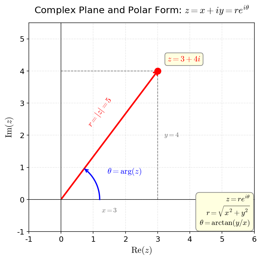
Fig. E.1: Complex plane and polar form representation. Figure E_1: Representation of the complex number \(z = x + iy = re^{i\theta}\) on the complex plane. Shows the real axis (horizontal), imaginary axis (vertical), distance from origin \(r = |z|\), and argument \(\theta = \arg(z)\) from the real axis.

Let's see why multiplication becomes simple. When \(z_1 = r_1 e^{i\theta_1}\), \(z_2 = r_2 e^{i\theta_2}\):

\[z_1 z_2 = r_1 e^{i\theta_1} \cdot r_2 e^{i\theta_2} = r_1 r_2 \, e^{i(\theta_1 + \theta_2)}\]

That is, absolute values multiply, arguments add. Geometrically, this is a composition of "rotation and scaling."

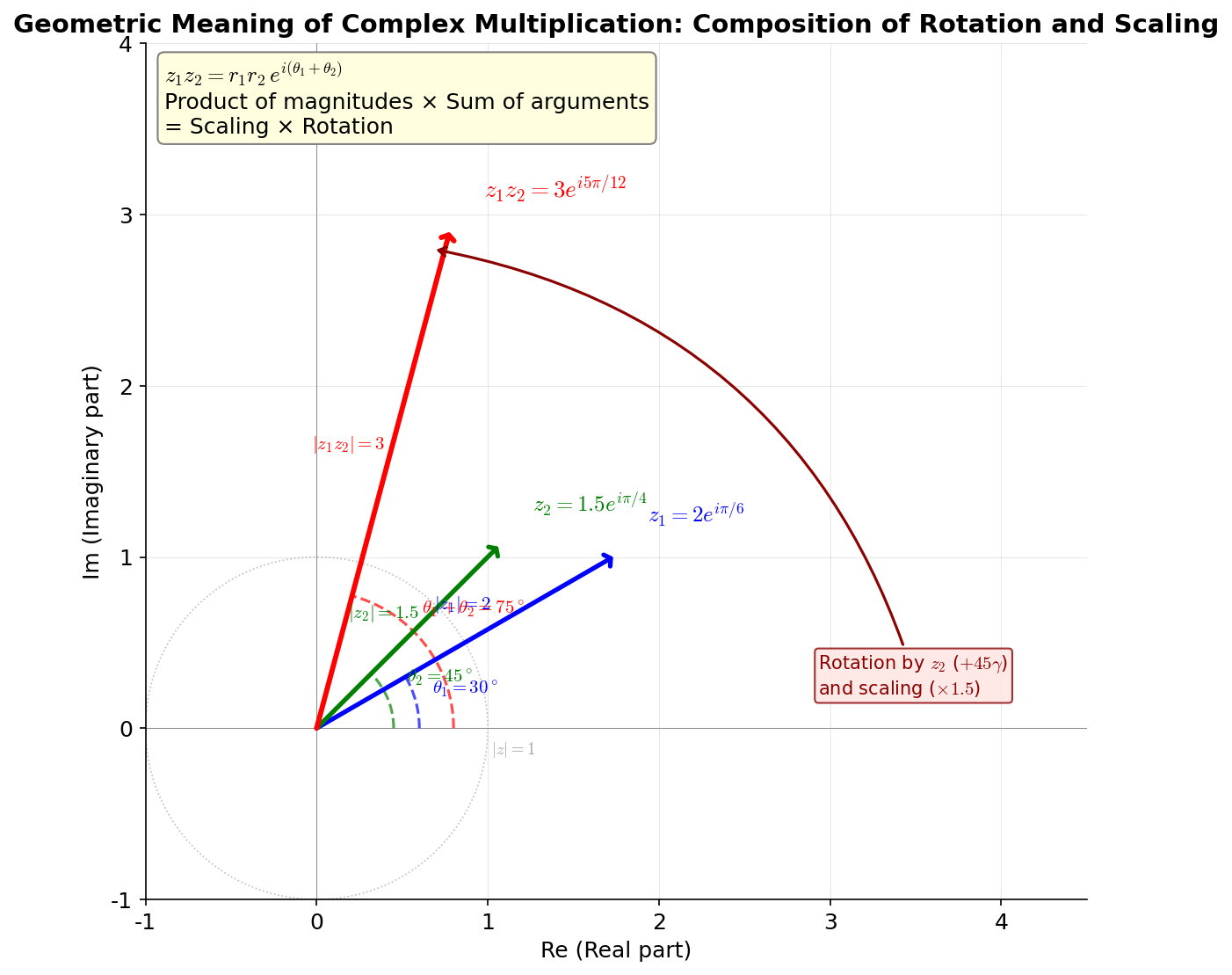
Fig. E.2: Geometric meaning of complex multiplication. Figure E_2: The product of two complex numbers \(z_1 = r_1 e^{i\theta_1}\), \(z_2 = r_2 e^{i\theta_2}\) has "product of absolute values, sum of arguments." Visualized as a composition of rotation and scaling.

🔵 Kai: What about division?

🟡 Lina: It becomes:

\[\frac{z_1}{z_2} = \frac{r_1}{r_2} e^{i(\theta_1 - \theta_2)}\]

Absolute values divide, arguments subtract.

📝 Exercises:

• Polar form and product of complex numbers → Problem B-1. Absolute Value and Argument of Complex Numbers, Problem B-3. Product in Polar Form

The Complex Plane

A complex number \(z = x + iy\) is represented as a point \((x, y)\) in a 2-dimensional plane. The horizontal axis is the real part (real axis), the vertical axis is the imaginary part (imaginary axis). \(|z|\) is the distance from the origin, \(\arg(z)\) is the counterclockwise angle from the real axis.

The Riemann Sphere — Adding the Point at Infinity

🟡 Lina: Let me introduce an important concept for conformal field theory. The complex plane with a single "point at infinity" \(z = \infty\) added is called the Riemann sphere \(\hat{\mathbb{C}} = \mathbb{C} \cup \{\infty\}\).

🔵 Kai: Infinity is a "point"?

🟡 Lina: Here's the geometric picture (Fig. E.3 "Stereographic projection and the Riemann sphere"). Place a unit sphere tangent to the complex plane, and draw a straight line from the north pole of the sphere to each point on the plane. The point where this line intersects the sphere corresponds to the complex number \(z\) on the sphere. The north pole itself corresponds to \(z = \infty\). This is called stereographic projection.

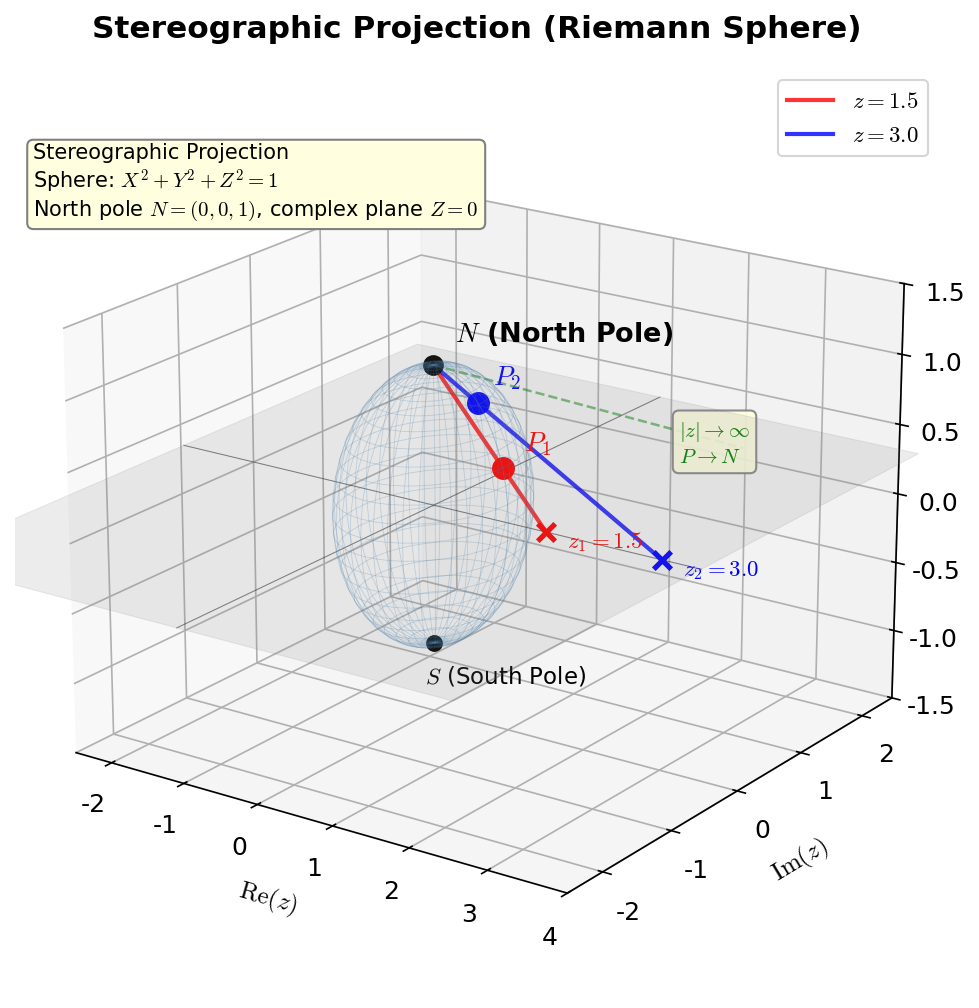
Fig. E.3: Stereographic projection and the Riemann sphere. Figure E_3: The point \(P\) where the line from the north pole \(N\) to the point \(z\) on the complex plane intersects the sphere corresponds to \(z\) on the sphere. As \(|z| \to \infty\), \(P \to N\) (north pole).

Let's derive this concretely. Consider the line connecting the north pole \(N = (0, 0, 1)\) and a point \(P = (X, Y, Z)\) on the sphere. As you learned with vectors in high school, points on the line through two points \(A\), \(B\) can be written as \(A + t(B - A)\) (\(t\) is a real parameter). When \(t = 0\) it equals point \(A\), when \(t = 1\) it equals point \(B\), and varying \(t\) moves along the line. With \(A = N = (0,0,1)\), \(B = P = (X,Y,Z)\), points on the line are \((0,0,1) + t((X,Y,Z) - (0,0,1)) = (tX, tY, 1 + t(Z-1))\). The condition for this line to intersect the \(Z = 0\) plane (complex plane) is \(1 + t(Z-1) = 0\), i.e., \(t = \frac{1}{1-Z}\). The coordinates of the intersection are \((x, y) = \left(\frac{X}{1-Z}, \frac{Y}{1-Z}\right)\), so:

\[z = x + iy = \frac{X + iY}{1 - Z}\]

🔵 Kai: As \(Z\) approaches 1 (points near the north pole), the denominator approaches 0, so \(|z|\) gets larger and larger.

🟡 Lina: Exactly. Conversely, to find \((X, Y, Z)\) from \(z\), use the unit sphere condition \(X^2 + Y^2 + Z^2 = 1\) (i.e., \(X^2 + Y^2 = 1 - Z^2\)) to get \(|z|^2 = \frac{X^2 + Y^2}{(1-Z)^2} = \frac{1-Z^2}{(1-Z)^2} = \frac{(1-Z)(1+Z)}{(1-Z)^2} = \frac{1+Z}{1-Z}\), giving \(Z = \frac{|z|^2 - 1}{|z|^2 + 1}\). Similarly:

\[X = \frac{z + \bar{z}}{|z|^2 + 1}, \quad Y = \frac{z - \bar{z}}{i(|z|^2 + 1)}, \quad Z = \frac{|z|^2 - 1}{|z|^2 + 1}\]

As \(|z| \to \infty\), \((X, Y, Z) \to (0, 0, 1)\) (north pole).

⚪ Mei: I see, so on the sphere, "infinity" becomes an ordinary point—the north pole.

🟡 Lina: Right. In Ch. 16, when compactifying the string worldsheet, this Riemann sphere appears naturally. When calculating string scattering amplitudes, the worldsheet topology becomes a sphere.

✅ Comprehension Check: How do you write the polar form of the complex number \(z = x + iy\)?

Answer

\(z = r e^{i\theta}\) (\(r = |z|\), \(\theta = \arg(z)\)).

✅ Comprehension Check: For two complex numbers in polar form \(z_1 = r_1 e^{i\theta_1}\), \(z_2 = r_2 e^{i\theta_2}\), what are the absolute value and argument of their product?

Answer

The absolute value is \(r_1 r_2\) (multiplication), the argument is \(\theta_1 + \theta_2\) (addition).

✅ Comprehension Check: What is the Riemann sphere?

Answer

The complex plane \(\mathbb{C}\) with a single point at infinity \(\infty\) added: \(\hat{\mathbb{C}} = \mathbb{C} \cup \{\infty\}\). It can be identified with a sphere via stereographic projection.

---

E.3　Complex Coordinates \(z, \bar{z}\) and Differentiation

Complex Coordinate Representation of the 2D Plane

🟡 Lina: Let me rewrite the 2-dimensional plane \((x, y)\) in complex coordinates.

\[z = x + iy, \qquad \bar{z} = x - iy\]

Solving inversely (from \(z + \bar{z} = 2x\), \(z - \bar{z} = 2iy\)):

\[x = \frac{z + \bar{z}}{2}, \qquad y = \frac{z - \bar{z}}{2i}\]

Transformation of Partial Derivatives

🔵 Kai: How do you convert the partial derivatives \(\partial_x, \partial_y\) in \((x, y)\) to partial derivatives in \((z, \bar{z})\)?

🟡 Lina: We use the chain rule. Viewing \(f\) as a function of \((z, \bar{z})\):

\[\frac{\partial f}{\partial x} = \frac{\partial f}{\partial z}\frac{\partial z}{\partial x} + \frac{\partial f}{\partial \bar{z}}\frac{\partial \bar{z}}{\partial x}\]

From \(z = x + iy\), \(\frac{\partial z}{\partial x} = 1\), and from \(\bar{z} = x - iy\), \(\frac{\partial \bar{z}}{\partial x} = 1\). Therefore:

\[\partial_x = \partial_z + \partial_{\bar{z}} \tag{E.1}\]

Similarly for \(y\):

\[\frac{\partial f}{\partial y} = \frac{\partial f}{\partial z}\frac{\partial z}{\partial y} + \frac{\partial f}{\partial \bar{z}}\frac{\partial \bar{z}}{\partial y}\]

Since \(\frac{\partial z}{\partial y} = i\) and \(\frac{\partial \bar{z}}{\partial y} = -i\):

\[\partial_y = i\partial_z - i\partial_{\bar{z}} \tag{E.2}\]

Solving equations (E.1) and (E.2) simultaneously for \(\partial_z\) and \(\partial_{\bar{z}}\). Computing (E.1) + (E.2)\(/i\):

\[\partial_x + \frac{\partial_y}{i} = \partial_z + \partial_{\bar{z}} + \partial_z - \partial_{\bar{z}} = 2\partial_z\]

Since \(\frac{1}{i} = -i\):

\[\partial_x - i\partial_y = 2\partial_z\]

\[\boxed{\partial_z \equiv \frac{\partial}{\partial z} = \frac{1}{2}(\partial_x - i\partial_y)} \tag{E.3}\]

Similarly (E.1) \(-\) (E.2)\(/i\):

\[\partial_x + i\partial_y = 2\partial_{\bar{z}}\]

\[\boxed{\partial_{\bar{z}} \equiv \frac{\partial}{\partial \bar{z}} = \frac{1}{2}(\partial_x + i\partial_y)} \tag{E.4}\]

⚪ Mei: Let me verify. \(\partial_z z = \frac{1}{2}(\partial_x - i\partial_y)(x + iy) = \frac{1}{2}(1 + 1) = 1\) ✓

\(\partial_z \bar{z} = \frac{1}{2}(\partial_x - i\partial_y)(x - iy) = \frac{1}{2}(1 - 1) = 0\) ✓

\(\partial_{\bar{z}} z = \frac{1}{2}(\partial_x + i\partial_y)(x + iy) = \frac{1}{2}(1 - 1) = 0\) ✓

\(\partial_{\bar{z}} \bar{z} = \frac{1}{2}(\partial_x + i\partial_y)(x - iy) = \frac{1}{2}(1 + 1) = 1\) ✓

🟡 Lina: Perfect. This confirms that \(z\) and \(\bar{z}\) formally behave as independent variables.

2D Laplacian

🟡 Lina: Let's rewrite the 2-dimensional Laplacian \(\nabla^2 = \partial_x^2 + \partial_y^2\) in complex coordinates.

From equations (E.1) and (E.2):

\[\partial_x^2 = (\partial_z + \partial_{\bar{z}})^2 = \partial_z^2 + 2\partial_z\partial_{\bar{z}} + \partial_{\bar{z}}^2\]

\[\partial_y^2 = (i\partial_z - i\partial_{\bar{z}})^2 = -\partial_z^2 + 2\partial_z\partial_{\bar{z}} - \partial_{\bar{z}}^2\]

Adding them:

\[\nabla^2 = \partial_x^2 + \partial_y^2 = 4\partial_z\partial_{\bar{z}}\]

\[\boxed{\nabla^2 = 4\frac{\partial^2}{\partial z \partial \bar{z}}} \tag{E.5}\]

🔵 Kai: The Laplacian factorizes into a product of \(\partial_z\) and \(\partial_{\bar{z}}\)! That's a very clean form, but... to be more specific, \(\nabla^2 \phi = 0\) is the same as \(\partial_z \partial_{\bar{z}} \phi = 0\), right? What form do the solutions of this equation take? Just because "the product is 0" doesn't mean "one factor is 0," right?

🟡 Lina: Good question. Think about this in two stages. Read the equation \(\partial_z \partial_{\bar{z}} \phi = 0\) as "\(\partial_z\) on the outside, \(\partial_{\bar{z}}\) on the inside," and first name \(\partial_{\bar{z}} \phi\) as \(h\). Then the equation becomes \(\partial_z h = 0\). This means "\(h\) doesn't depend on \(z\)," so \(h\) is a function of \(\bar{z}\) only: \(h = h(\bar{z})\). Next, integrating \(\partial_{\bar{z}} \phi = h(\bar{z})\) with respect to \(\bar{z}\) gives \(\phi = g(\bar{z}) + f(z)\). Here \(g(\bar{z})\) is a primitive function of \(h(\bar{z})\), and \(f(z)\) plays the role of an integration constant as a function of \(z\) alone.

🔵 Kai: Ah, I see. Just like integrating \(\frac{d}{dx}F(x) = h(x)\) in real calculus gives \(F(x) = \int h\,dx + C\) with a constant \(C\), here instead of a "constant" we get "an arbitrary function of \(z\) alone, \(f(z)\)." So when integrating with respect to \(\bar{z}\), \(z\) is treated as a "constant," and the integration constant becomes an arbitrary function of \(z\).

🟡 Lina: Exactly. So the general solution of the 2-dimensional Laplace equation is \(\phi = f(z) + g(\bar{z})\), completely separating into holomorphic and anti-holomorphic parts. This is very important in Ch. 16 and is the core reason why conformal field theory calculations split into left-moving and right-moving modes.

⚪ Mei: I see, so mathematically "the Laplacian factorizes into \(\partial_z \partial_{\bar{z}}\)" corresponds physically to "the holomorphic and anti-holomorphic parts completely separate." What Lina called "the core reason why CFT calculations split into left and right modes" is precisely this factorization.

📝 Exercises:

• Verification of partial derivatives in complex coordinates → Problem B-6. \(\partial_z(z^2) = 2z\)

Why Treat \(z\) and \(\bar{z}\) as Independent

🔵 Kai: Wait a moment. \(\bar{z}\) is determined by the complex conjugate of \(z\), right? Is it okay to treat it as an independent variable? The actual degrees of freedom are 2 from \((x, y)\), but treating \((z, \bar{z})\) as 2 variables makes it seem like the degrees of freedom increased.

🟡 Lina: Good question. Let me use an analogy. It's like specifying a position on a map using "distance in the northeast direction" and "distance in the northwest direction" instead of "latitude and longitude." Both carry the same information, but choosing coordinates that match the symmetry of the problem makes calculations easier.

🔵 Kai: Hmm, but that's "just a change of perspective" and doesn't actually add independent variables, right? If \(\bar{z}\) is determined by \(z\), then what does "holding \(\bar{z}\) fixed and varying only \(z\)" mean physically?

🟡 Lina: You're right—\(\bar{z}\) is the complex conjugate of \(z\), so once \(z\) is determined, \(\bar{z}\) is also determined—physically they're not independent. But as a computational tool, treating \(z\) and \(\bar{z}\) as "separate variables" and defining partial derivatives leads to no contradictions. The justification appears in the relations we verified above: \(\partial_z \bar{z} = 0\), \(\partial_{\bar{z}} z = 0\). The differentiation rule "\(\bar{z}\) doesn't change when you vary \(z\)" holds, so computationally they can be treated just like independent variables. When computing physical quantities at the end, you just restore the relation \(\bar{z} = z^*\).

In the conformal field theory of Ch. 16, the part depending on \(z\) (holomorphic part) and the part depending on \(\bar{z}\) (anti-holomorphic part) separate, and each can be analyzed independently. This is one reason CFT calculations are so powerful.

2D Line Element and Area Form

🟡 Lina: Since we'll use it later, let me also write the metric in complex coordinates.

The line element in real coordinates is \(ds^2 = dx^2 + dy^2\). Substituting \(dx = \frac{1}{2}(dz + d\bar{z})\), \(dy = \frac{1}{2i}(dz - d\bar{z})\):

\[ds^2 = dx^2 + dy^2 = \frac{1}{4}(dz + d\bar{z})^2 + \frac{1}{(2i)^2}(dz - d\bar{z})^2\]

Since \((2i)^2 = 4i^2 = -4\), we have \(\frac{1}{(2i)^2} = -\frac{1}{4}\). Therefore:

\[ds^2 = \frac{1}{4}(dz + d\bar{z})^2 + \left(-\frac{1}{4}\right)(dz - d\bar{z})^2 = \frac{1}{4}(dz + d\bar{z})^2 - \frac{1}{4}(dz - d\bar{z})^2\]

Expanding (where the product here is the symmetric product of the metric tensor \(dz\,d\bar{z} = d\bar{z}\,dz\), different from the antisymmetric wedge product \(dz \wedge d\bar{z} = -d\bar{z} \wedge dz\) that appears later):

\[= \frac{1}{4}(dz^2 + 2dz\,d\bar{z} + d\bar{z}^2) - \frac{1}{4}(dz^2 - 2dz\,d\bar{z} + d\bar{z}^2)\]

\[= \frac{1}{4} \cdot 4 \, dz\,d\bar{z} = dz\,d\bar{z}\]

\[\boxed{ds^2 = dz\,d\bar{z}} \tag{E.6}\]

⚪ Mei: The \(dz^2\) and \(d\bar{z}^2\) terms cancel cleanly, leaving only the cross term.

🟡 Lina: Let me also write the area element in complex coordinates:

\[d^2z \equiv dx\,dy = \frac{i}{2} dz \wedge d\bar{z} \tag{E.7}\]

Here \(d^2z\) is not "\(dz\) squared" but an abbreviation for the "2-dimensional area element." The superscript 2 indicates the dimension (in 3 dimensions it would be \(d^3x = dx\,dy\,dz\)). The wedge product \(\wedge\) on the right makes explicit that swapping the order of \(dz\) and \(d\bar{z}\) changes the sign. In practice, think of it as "\(dx\,dy\) rewritten in complex coordinates."

🔵 Kai: What's \(\wedge\)? Is it different from ordinary multiplication?

🟡 Lina: \(\wedge\) (wedge product) is a "product that creates oriented area elements." The reason we need this instead of ordinary multiplication is that we want to correctly track the sign (orientation) of area under coordinate transformations. With ordinary multiplication \(dx \cdot dy\), there's no distinction between "\(x\) first or \(y\) first," but the wedge product maintains orientation information through its antisymmetry \(A \wedge B = -B \wedge A\).

Why antisymmetric? Because area has "orientation." For example, moving 1 unit in the \(x\)-direction then 1 unit in the \(y\)-direction creates a counterclockwise unit square, but moving in the \(y\)-direction first then \(x\)-direction gives clockwise. The wedge product distinguishes this "direction of traversal" by sign. That is, \(dx \wedge dy = -dy \wedge dx\).

The \(dx\,dy\) used in ordinary area integrals \(\int dx\,dy\) is actually \(dx \wedge dy\) (oriented area element with counterclockwise as positive). When orientation doesn't matter, we simply write \(dx\,dy\), but when tracking signs under coordinate transformations, wedge product notation is convenient. In this appendix, unless otherwise stated, we use \(dx\,dy\) and \(dx \wedge dy\) with the same meaning.

🔵 Kai: If it's antisymmetric, what happens with \(A \wedge A\)?

🟡 Lina: From the antisymmetry \(A \wedge B = -B \wedge A\), setting \(B = A\) gives \(A \wedge A = -A \wedge A\). Adding \(A \wedge A\) to both sides gives \(2(A \wedge A) = 0\). Therefore \(A \wedge A = 0\). The wedge product of identical forms is always 0.

⚪ Mei: I see, so \(dz \wedge dz = 0\), \(d\bar{z} \wedge d\bar{z} = 0\), and when expanding, all "same with same" terms vanish.

🟡 Lina: Exactly. Now let's actually compute the area element. Substituting \(dx = \frac{1}{2}(dz + d\bar{z})\), \(dy = \frac{1}{2i}(dz - d\bar{z})\):

\[dx \wedge dy = \frac{1}{2} \cdot \frac{1}{2i}(dz + d\bar{z}) \wedge (dz - d\bar{z}) = \frac{1}{4i}(dz \wedge dz - dz \wedge d\bar{z} + d\bar{z} \wedge dz - d\bar{z} \wedge d\bar{z})\]

By antisymmetry, \(dz \wedge dz = 0\), \(d\bar{z} \wedge d\bar{z} = 0\), \(d\bar{z} \wedge dz = -dz \wedge d\bar{z}\), so:

\[dx \wedge dy = \frac{1}{4i}(-2\, dz \wedge d\bar{z}) = -\frac{1}{2i}\, dz \wedge d\bar{z} = \frac{i}{2}\, dz \wedge d\bar{z}\]

(Final equality: used \(-\frac{1}{2i} = -\frac{1}{2i}\cdot\frac{i}{i} = -\frac{i}{2i^2} = -\frac{i}{-2} = \frac{i}{2}\).)

🔵 Kai: It matches equation (E.7) exactly! You just mechanically follow the wedge product rules and it comes out.

✅ Comprehension Check: How do you express the partial derivative \(\partial_z\) in terms of \(\partial_x\) and \(\partial_y\)?

Answer

\(\partial_z = \frac{1}{2}(\partial_x - i\partial_y)\).

✅ Comprehension Check: How do you write the 2-dimensional Laplacian \(\nabla^2 = \partial_x^2 + \partial_y^2\) in complex coordinates?

Answer

\(\nabla^2 = 4\partial_z\partial_{\bar{z}}\).

✅ Comprehension Check: What is the advantage of formally treating \(z\) and \(\bar{z}\) as independent variables in conformal field theory?

Answer

The holomorphic part depending on \(z\) and the anti-holomorphic part depending on \(\bar{z}\) separate, allowing each to be analyzed independently, making calculations concise.

---

E.4　Holomorphic Functions and the Cauchy-Riemann Conditions

Definition

🟡 Lina: A complex function \(f(z, \bar{z})\) is holomorphic if it does not depend on \(\bar{z}\):

\[\frac{\partial f}{\partial \bar{z}} = 0 \tag{E.8}\]

That is, \(f\) is a function of \(z\) alone: \(f = f(z)\).

Derivation of the Cauchy-Riemann Conditions

🔵 Kai: What happens when you separate this into real and imaginary parts?

🟡 Lina: Write \(f(z) = u(x,y) + iv(x,y)\) and expand \(\partial_{\bar{z}} f = 0\).

Using the definition from equation (E.4), \(\partial_{\bar{z}} = \frac{1}{2}(\partial_x + i\partial_y)\):

\[\partial_{\bar{z}} f = \frac{1}{2}(\partial_x + i\partial_y)(u + iv)\]

Expanding:

\[= \frac{1}{2}\left(\frac{\partial u}{\partial x} + i\frac{\partial v}{\partial x} + i\frac{\partial u}{\partial y} + i^2\frac{\partial v}{\partial y}\right)\]

Using \(i^2 = -1\) and organizing:

\[= \frac{1}{2}\left(\frac{\partial u}{\partial x} - \frac{\partial v}{\partial y}\right) + \frac{i}{2}\left(\frac{\partial v}{\partial x} + \frac{\partial u}{\partial y}\right)\]

For this to be 0, the real and imaginary parts must each be 0:

\[\frac{\partial u}{\partial x} - \frac{\partial v}{\partial y} = 0\]

\[\frac{\partial v}{\partial x} + \frac{\partial u}{\partial y} = 0\]

Rearranging:

\[\boxed{\frac{\partial u}{\partial x} = \frac{\partial v}{\partial y}, \qquad \frac{\partial u}{\partial y} = -\frac{\partial v}{\partial x}} \tag{E.9}\]

These are the Cauchy-Riemann relations.

⚪ Mei: So the real and imaginary parts of a holomorphic function aren't independent—they're connected by these relations.

🟡 Lina: Right. There's an important further consequence. Differentiating the first Cauchy-Riemann equation with respect to \(x\) and the second with respect to \(y\):

\[\frac{\partial^2 u}{\partial x^2} = \frac{\partial^2 v}{\partial x \partial y}, \qquad \frac{\partial^2 u}{\partial y^2} = -\frac{\partial^2 v}{\partial y \partial x}\]

Using the equality of mixed partial derivatives of \(v\) (\(\frac{\partial^2 v}{\partial x \partial y} = \frac{\partial^2 v}{\partial y \partial x}\)) and adding:

\[\frac{\partial^2 u}{\partial x^2} + \frac{\partial^2 u}{\partial y^2} = 0\]

That is, the real part \(u\) of a holomorphic function satisfies the Laplace equation (it's a harmonic function). Similarly, the imaginary part \(v\) is also harmonic.

🔵 Kai: Wait, just being holomorphic automatically means it satisfies the Laplace equation? That's a strong constraint...

Verification with Concrete Examples

🟡 Lina: Let's verify the Cauchy-Riemann conditions with several functions.

Example 1: \(f(z) = z^2 = (x+iy)^2 = x^2 - y^2 + 2ixy\)

With \(u = x^2 - y^2\), \(v = 2xy\):

\[\frac{\partial u}{\partial x} = 2x, \quad \frac{\partial v}{\partial y} = 2x \quad \checkmark\]

\[\frac{\partial u}{\partial y} = -2y, \quad -\frac{\partial v}{\partial x} = -2y \quad \checkmark\]

Example 2: \(f(z) = e^z = e^{x+iy} = e^x(\cos y + i\sin y)\)

With \(u = e^x \cos y\), \(v = e^x \sin y\):

\[\frac{\partial u}{\partial x} = e^x \cos y, \quad \frac{\partial v}{\partial y} = e^x \cos y \quad \checkmark\]

\[\frac{\partial u}{\partial y} = -e^x \sin y, \quad -\frac{\partial v}{\partial x} = -e^x \sin y \quad \checkmark\]

Example 3 (non-holomorphic): \(f(z) = |z|^2 = z\bar{z} = x^2 + y^2\)

With \(u = x^2 + y^2\), \(v = 0\):

\[\frac{\partial u}{\partial x} = 2x, \quad \frac{\partial v}{\partial y} = 0\]

Since \(2x \neq 0\) (in general), the Cauchy-Riemann conditions are not satisfied. This is expected since it depends on \(\bar{z}\).

Table E.2: Determination of holomorphicity for representative functions

Function	Holomorphic?	Reason
\(f(z) = z^n\)	✓	Does not depend on \(\bar{z}\)
\(f(z) = e^z\)	✓	Satisfies CR relations
\(f(z) = 1/z\)	✓ (for \(z \neq 0\))	Singularity at \(z = 0\)
$f(z) =	z	^2 = z\bar{z}$
\(f(z) = \bar{z}\)	✗	\(\partial_{\bar{z}}\bar{z} = 1 \neq 0\)
> 📝 Exercises:
>
> - Verification of Cauchy-Riemann relations → Problem B-4. Cauchy-Riemann: Verification with \(z^2\), [Problem B-5. Cauchy-Riemann: $	z	^2$ Fails](../problems/appendix_e.md#string-appe-cr-fails-mod-z-squared)

Holomorphic Functions as Conformal Maps

🟡 Lina: Holomorphic functions have a geometrically very important property. When \(w = f(z)\) is holomorphic and \(f'(z_0) \neq 0\), this map preserves angles (is conformal).

🔵 Kai: What does "preserves angles" mean?

🟡 Lina: When two curves passing through point \(z_0\) intersect at angle \(\alpha\), the two curves after mapping by \(f\) also intersect at the same angle \(\alpha\).

Let me show this. Consider a curve \(z(t)\) passing through \(z_0\). The mapped curve is \(w(t) = f(z(t))\). The tangent vector is:

\[\frac{dw}{dt} = f'(z) \frac{dz}{dt}\]

Writing \(f'(z_0) = |f'(z_0)| e^{i\phi}\) in polar form, the argument of the tangent vector is:

\[\arg\left(\frac{dw}{dt}\right) = \phi + \arg\left(\frac{dz}{dt}\right)\]

That is, all directions are uniformly rotated by angle \(\phi\). The angle between two curves doesn't change.

⚪ Mei: So summarizing Lina's explanation, since all directions rotate by the same angle, the angles between curves are preserved.

🟡 Lina: This is why conformal transformations are described by holomorphic functions in Ch. 16. "Conformal" = "angle-preserving" = "holomorphic."

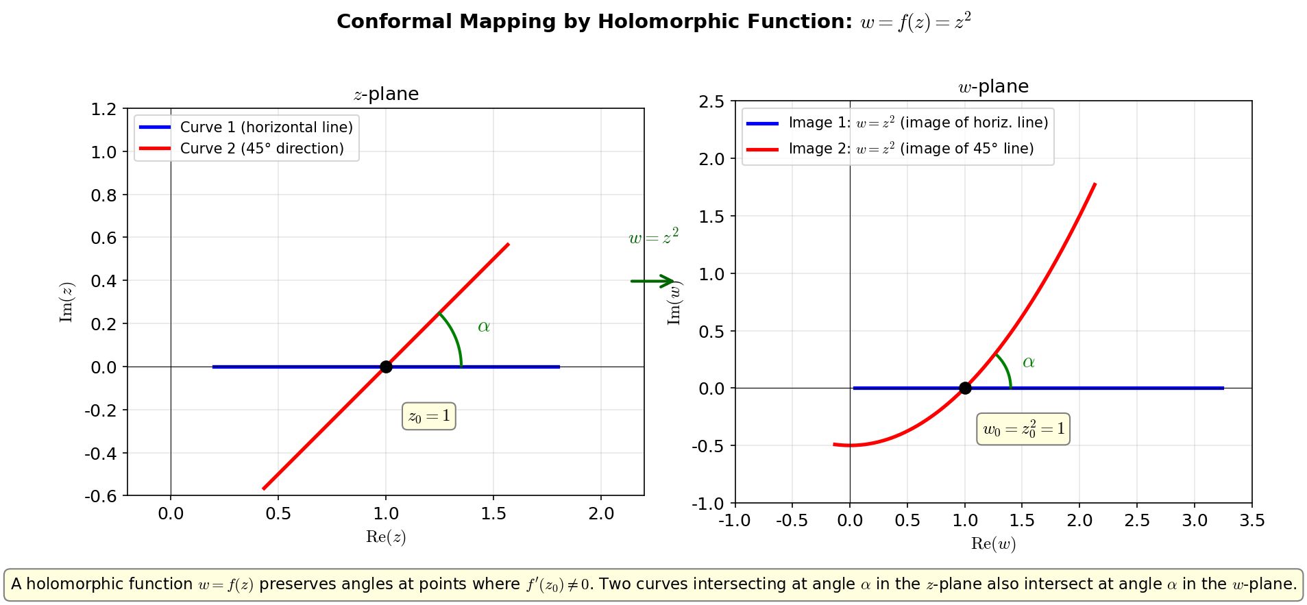
Fig. E.4: Conformal mapping by a holomorphic function. Figure E_4: A holomorphic function \(w = f(z)\) preserves angles. Two curves intersecting at angle \(\alpha\) in the \(z\)-plane also intersect at the same angle \(\alpha\) in the \(w\)-plane.

📝 Exercises:

• Concrete example of conformal mapping → Problem A-1. Conformal Mapping \(w = 1/z\)

✅ Comprehension Check: How do you write the condition for a complex function \(f(z, \bar{z})\) to be holomorphic using partial derivatives?

Answer

\(\partial_{\bar{z}} f = 0\) (\(f\) does not depend on \(\bar{z}\)).

✅ Comprehension Check: How do you write the Cauchy-Riemann conditions in terms of the real and imaginary parts of \(f = u + iv\)?

Answer

\(\frac{\partial u}{\partial x} = \frac{\partial v}{\partial y}\), \(\frac{\partial u}{\partial y} = -\frac{\partial v}{\partial x}\).

✅ Comprehension Check: What geometric property does the map by a holomorphic function \(w = f(z)\) (\(f'(z_0) \neq 0\)) have?

Answer

It is an angle-preserving map (conformal map).

---

E.5　Conformal Maps and Conformal Transformations

Möbius Transformations

🟡 Lina: The most important class of conformal transformations is the Möbius transformation (linear fractional transformation):

\[\boxed{w = \frac{az + b}{cz + d}, \qquad ad - bc \neq 0} \tag{E.10}\]

Here \(a, b, c, d\) are complex constants.

🔵 Kai: Why is \(ad - bc \neq 0\) necessary?

🟡 Lina: When \(ad - bc = 0\), \(w\) becomes a constant (the map degenerates). Let's verify. When \(ad = bc\), we have \(\frac{a}{c} = \frac{b}{d}\), so:

\[w = \frac{az + b}{cz + d} = \frac{a(z + b/a)}{c(z + d/c)} = \frac{a}{c} \cdot \frac{z + b/a}{z + b/a} = \frac{a}{c}\]

(Used \(b/a = d/c\).) A constant map loses information, so we exclude it.

Derivative and Conformality of Möbius Transformations

Computing the derivative of \(w = f(z) = \frac{az+b}{cz+d}\):

\[f'(z) = \frac{a(cz+d) - c(az+b)}{(cz+d)^2} = \frac{acz + ad - acz - bc}{(cz+d)^2} = \frac{ad - bc}{(cz+d)^2}\]

Since \(ad - bc \neq 0\) and \(cz + d \neq 0\) imply \(f'(z) \neq 0\), it is indeed a conformal map.

Möbius Transformations and Matrices

🟡 Lina: Möbius transformations correspond to \(2 \times 2\) matrices:

\[w = \frac{az+b}{cz+d} \quad \longleftrightarrow \quad M = \begin{pmatrix} a & b \\ c & d \end{pmatrix}\]

The composition of two Möbius transformations corresponds to matrix multiplication. Let's verify.

Applying \(w_1 = \frac{a_1 z + b_1}{c_1 z + d_1}\) followed by \(w_2 = \frac{a_2 w + b_2}{c_2 w + d_2}\):

\[w_2 = \frac{a_2 \cdot \frac{a_1 z + b_1}{c_1 z + d_1} + b_2}{c_2 \cdot \frac{a_1 z + b_1}{c_1 z + d_1} + d_2}\]

Multiplying numerator and denominator by \((c_1 z + d_1)\):

\[= \frac{a_2(a_1 z + b_1) + b_2(c_1 z + d_1)}{c_2(a_1 z + b_1) + d_2(c_1 z + d_1)} = \frac{(a_2 a_1 + b_2 c_1)z + (a_2 b_1 + b_2 d_1)}{(c_2 a_1 + d_2 c_1)z + (c_2 b_1 + d_2 d_1)}\]

This is exactly the Möbius transformation corresponding to the matrix product:

\[M_2 M_1 = \begin{pmatrix} a_2 & b_2 \\ c_2 & d_2 \end{pmatrix}\begin{pmatrix} a_1 & b_1 \\ c_1 & d_1 \end{pmatrix} = \begin{pmatrix} a_2 a_1 + b_2 c_1 & a_2 b_1 + b_2 d_1 \\ c_2 a_1 + d_2 c_1 & c_2 b_1 + d_2 d_1 \end{pmatrix}\]

🔵 Kai: If composition is matrix multiplication, is there also an inverse transformation? Like how matrices have inverse matrices.

🟡 Lina: Good insight. The inverse transformation corresponds to the inverse matrix, and the identity transformation (doing nothing) corresponds to the identity matrix.

⚪ Mei: So the set of all Möbius transformations is closed under matrix multiplication. Composing them always gives another Möbius transformation.

🔵 Kai: Closed under composition, inverses exist, identity exists... it feels like everything fits together. Is that a coincidence?

🟡 Lina: Not a coincidence. A structure that is "closed under composition, with inverses and an identity element" is called a group in mathematics (discussed in detail in Appendix D). Strictly speaking, "associativity" is also needed—meaning \((f \circ g) \circ h = f \circ (g \circ h)\) (composing three transformations gives the same result regardless of grouping)—but matrix multiplication satisfies associativity, so it's automatically OK.

🟡 Lina: Furthermore, matrices \(M\) and \(\lambda M\) (\(\lambda \neq 0\)) give the same Möbius transformation (since \(\lambda\) multiplies both numerator and denominator and cancels). So we can normalize to \(\det M = ad - bc = 1\). The set of all \(2\times 2\) complex matrices satisfying this condition is written \(\text{SL}(2, \mathbb{C})\) (SL stands for Special Linear, the special linear group with "determinant = 1").

🔵 Kai: Even though scaling by \(\lambda\) gives the same transformation, you can fix the determinant to 1?

🟡 Lina: Choosing \(\lambda = 1/\sqrt{\det M}\) gives \(\det(\lambda M) = \lambda^2 \det M = 1\). However, there's still freedom in the sign of \(\lambda\). That is, matrices \(M\) and \(-M\) give the same Möbius transformation (the signs in numerator and denominator cancel). So the group that identifies \(\pm I\) (\(I\) is the identity matrix) is:

\[\text{Group of Möbius transformations} \cong \text{SL}(2, \mathbb{C}) / \{\pm I\} = \text{PSL}(2, \mathbb{C})\]

(PSL stands for Projective Special Linear. "Projective" means "treating overall constant multiples as the same," which here corresponds to "identifying \(M\) and \(-M\) as the same transformation." You don't need to memorize the name—what matters is the structure "Group of Möbius transformations ≅ \(\text{SL}(2, \mathbb{C})/\{\pm I\}\)".)

Special Cases of Möbius Transformations

🟡 Lina: Möbius transformations can be written as compositions of 3 basic operations:

1. Translation: \(w = z + b\) (\(a=1, c=0, d=1\))
2. Rotation and scaling: \(w = az\) (\(b=0, c=0, d=1\))
3. Inversion: \(w = 1/z\) (\(a=0, b=1, c=1, d=0\))

🔵 Kai: You can build all Möbius transformations from just 3 types of operations?

🟡 Lina: Yes. A general Möbius transformation with \(c \neq 0\) can be decomposed by splitting the numerator \(az + b\) into a constant multiple of \(cz + d\) and a remainder (if \(c = 0\) then \(w = (a/d)z + b/d\) is simply rotation/scaling + translation):

\[\frac{az+b}{cz+d} = \frac{a}{c} + \frac{b - ad/c}{cz+d} = \frac{a}{c} + \frac{bc-ad}{c(cz+d)} = \frac{a}{c} + \frac{bc-ad}{c^2} \cdot \frac{1}{z + d/c}\]

(First equality: decomposed the numerator as \(az + b = \frac{a}{c}(cz+d) + (b - \frac{ad}{c})\). Check: \(\frac{a}{c}(cz+d) = az + \frac{ad}{c}\), so the remainder is \(az + b - az - \frac{ad}{c} = b - \frac{ad}{c}\) ✓. Second equality: used \(b - ad/c = (bc - ad)/c\).)

Reading this final form as a sequence of operations on \(z\):

1. First translate \(z\) by \(d/c\): \(z \mapsto z + d/c\)
2. Invert: \(z + d/c \mapsto \frac{1}{z + d/c}\)
3. Scale and rotate (multiply by coefficient \(\frac{bc-ad}{c^2}\)): \(\frac{1}{z+d/c} \mapsto \frac{bc-ad}{c^2} \cdot \frac{1}{z+d/c}\)
4. Finally translate by \(a/c\): \(\mapsto \frac{a}{c} + \frac{bc-ad}{c^2} \cdot \frac{1}{z+d/c}\)

So any Möbius transformation can be written as a composition of "translation → inversion → scaling/rotation → translation." (Note that \(bc - ad = -(ad - bc) \neq 0\), so the coefficient in step 3 is never zero. It's just a sign flip, with the non-degeneracy condition \(ad - bc \neq 0\) ensuring this.)

⚪ Mei: So even a seemingly complex Möbius transformation can be understood by decomposing it into the 3 basic operations.

Connection to String Theory

🟡 Lina: As you'll learn in Ch. 16, the global conformal transformations on the string worldsheet are described by Möbius transformations (\(\text{SL}(2, \mathbb{C})\)). When computing string scattering amplitudes, the freedom of Möbius transformations can be used to fix the positions of 3 vertex operators. This is called "\(\text{SL}(2, \mathbb{C})\) gauge fixing."

✅ Comprehension Check: What is the non-degeneracy condition for the Möbius transformation \(w = \frac{az+b}{cz+d}\)?

Answer

\(ad - bc \neq 0\).

📝 Exercises:

• Composition of Möbius transformations → Problem M-3. Composition of Möbius Transformations

✅ Comprehension Check: The composition of two Möbius transformations corresponds to what operation on the corresponding matrices?

Answer

It corresponds to matrix multiplication.

---

E.6　Taylor Expansion and Laurent Expansion

Taylor Expansion

🟡 Lina: A holomorphic function can be Taylor expanded in its region of holomorphicity:

\[f(z) = \sum_{n=0}^{\infty} a_n (z - z_0)^n, \qquad a_n = \frac{f^{(n)}(z_0)}{n!} \tag{E.11}\]

The range where this series converges is the interior of a disk centered at \(z_0\). The radius of that disk (radius of convergence) is determined by the distance from \(z_0\) to the nearest singularity. Intuitively, the function is "smooth" until reaching a singularity so it can be represented by a series, but at the singularity the function diverges so the series breaks down.

The Need for Laurent Expansion

🔵 Kai: What do we do with functions that have singularities? \(1/z\) diverges at \(z = 0\) so it can't be Taylor expanded, right?

🟡 Lina: Right. For functions with singularities, we need Laurent expansion which includes negative powers:

\[\boxed{f(z) = \sum_{n=-\infty}^{\infty} a_n (z - z_0)^n} \tag{E.12}\]

Laurent Expansion Coefficients

🟡 Lina: How are the coefficients \(a_n\) determined? Let me derive this.

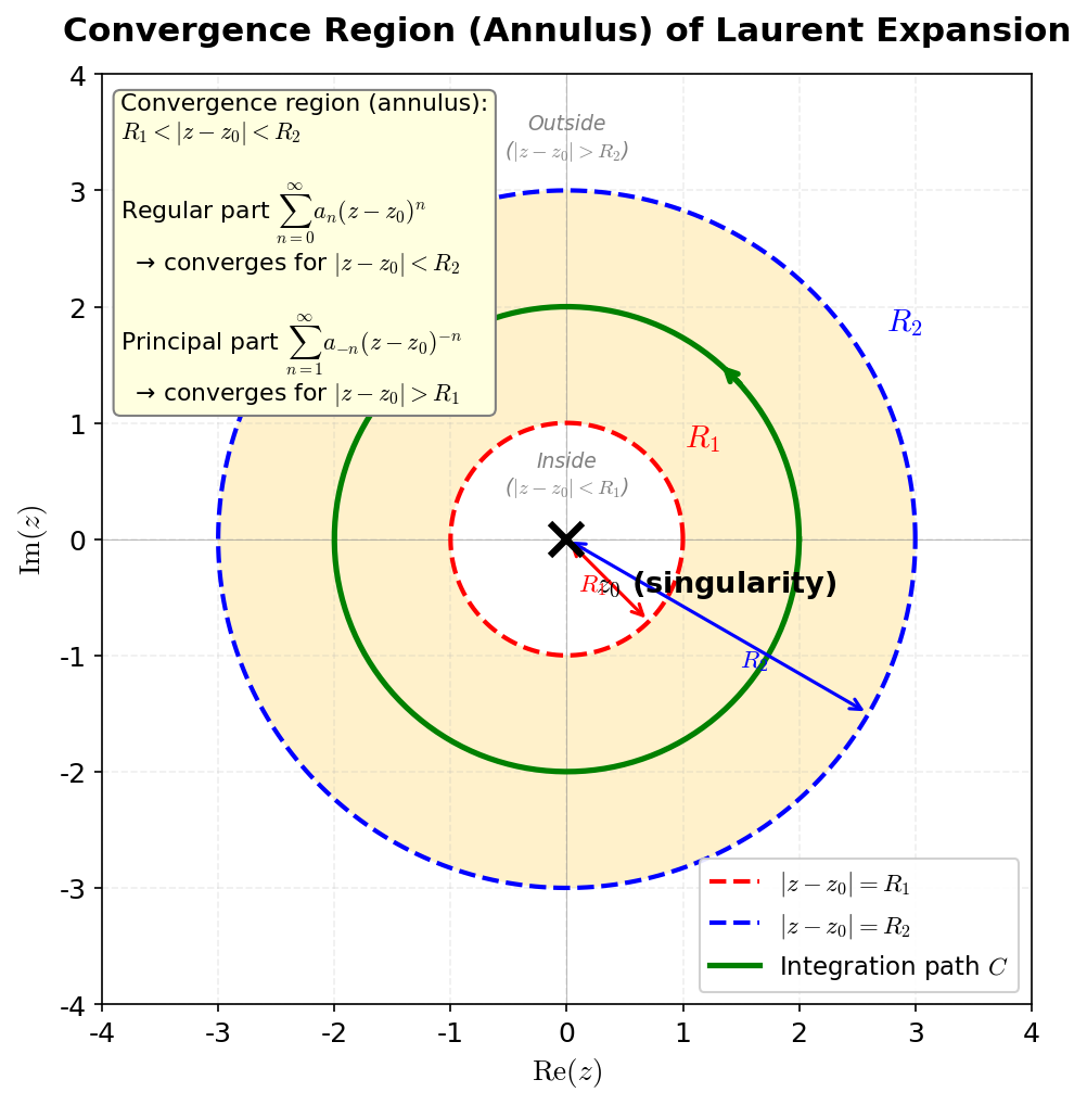
Fig. E.5: Convergence annulus for Laurent expansion. Figure E_5: The Laurent expansion converges in the annular region \(R_1 < |z - z_0| < R_2\) surrounding the singularity \(z_0\). The regular part converges inside the outer circle, and the principal part converges outside the inner circle.

Assume \(f\) is holomorphic in the annular region (annulus) between two concentric circles \(C_1\) (radius \(R_1\)) and \(C_2\) (radius \(R_2 > R_1\)) centered at \(z_0\).

The formula for Laurent coefficients is derived from Cauchy's integral formula in E.7 "Cauchy's Integral Formula and the Residue Theorem" (the idea, stated in advance: multiply the Laurent expansion by \((w-z_0)^{-n-1}\) on \(C\) and integrate term by term. Integrals of the form \(\oint_C (w-z_0)^{m-n-1}dw\) appear, which are \(2\pi i\) only when \(m = n\) and 0 otherwise, so only the \(a_n\) term survives).

🔵 Kai: "Non-zero only when \(m = n\)" — is that the same mechanism as in Fourier expansion where integrating the product of \(e^{im\theta}\) and \(e^{-in\theta}\) leaves something only when \(m = n\)?

🟡 Lina: Exactly! Let's verify this "orthogonality" concretely. Parametrizing as \(w = z_0 + re^{i\theta}\) (\(0 \leq \theta \leq 2\pi\)) gives \(dw = ire^{i\theta}d\theta\), \((w-z_0)^k = r^k e^{ik\theta}\), so:

\[\oint_C (w-z_0)^k\,dw = \int_0^{2\pi} r^k e^{ik\theta}\cdot ir e^{i\theta}\,d\theta = ir^{k+1}\int_0^{2\pi} e^{i(k+1)\theta}\,d\theta\]

When \(k+1 \neq 0\) (i.e., \(k \neq -1\)), since \(e^{i(k+1)\theta} = \cos((k+1)\theta) + i\sin((k+1)\theta)\), we have \(\int_0^{2\pi} e^{i(k+1)\theta}d\theta = \int_0^{2\pi}\cos((k+1)\theta)\,d\theta + i\int_0^{2\pi}\sin((k+1)\theta)\,d\theta\). Both \(\cos\) and \(\sin\) contain an integer number of complete periods, so positive and negative parts cancel, and both integrals are 0. When \(k = -1\), \(e^{i \cdot 0 \cdot \theta} = 1\) so \(\int_0^{2\pi} 1\,d\theta = 2\pi\). The result is \(i r^0 \cdot 2\pi = 2\pi i\).

That is: \(\oint_C (w-z_0)^k\,dw = \begin{cases} 2\pi i & (k = -1) \\ 0 & (k \neq -1) \end{cases}\)

⚪ Mei: So this is the complex version of "orthogonality." Only \(k = -1\) survives, which corresponds to the \(\delta_{mn}\) in Fourier analysis.

🟡 Lina: This is the same mechanism as the orthogonality of trigonometric functions (the property that \(\int_0^{2\pi} \cos(m\theta)\cos(n\theta)\,d\theta\) is non-zero only when \(m = n\)), generalized in Fourier series as the "orthogonality" where \(\int_0^{2\pi} e^{ik\theta} e^{-il\theta} d\theta\) is non-zero only when \(k = l\). Let me state the result first so you can get used to using it. On the circle \(C\) of radius \(r\) (\(R_1 < r < R_2\)) centered at \(z_0\):

\[a_n = \frac{1}{2\pi i} \oint_C \frac{f(w)}{(w - z_0)^{n+1}} dw \tag{E.13}\]

⚪ Mei: Is this consistent with the Taylor expansion coefficient \(a_n = f^{(n)}(z_0)/n!\) when \(n \geq 0\)?

🟡 Lina: Good question. If \(f\) is holomorphic at \(z_0\), then from Cauchy's integral formula shown later:

\[f^{(n)}(z_0) = \frac{n!}{2\pi i} \oint_C \frac{f(w)}{(w-z_0)^{n+1}} dw\]

so \(a_n = f^{(n)}(z_0)/n!\) indeed agrees.

Structure of the Laurent Expansion

• The \(n \geq 0\) part: regular part (analytic part)

\[\sum_{n=0}^{\infty} a_n (z - z_0)^n\]

• The \(n < 0\) part: principal part

\[\sum_{n=1}^{\infty} a_{-n} (z - z_0)^{-n} = \frac{a_{-1}}{z-z_0} + \frac{a_{-2}}{(z-z_0)^2} + \cdots\]

The principal part describes the structure of the singularity.

Classification of Singularities

Table E.3: Classification of singularities of complex functions

Type	Condition	Example
Removable singularity	No principal part (\(a_n = 0\) for all \(n < 0\))	\(\frac{\sin z}{z}\) at \(z = 0\)
Pole of order \(N\)	\(a_{-N} \neq 0\), \(a_n = 0\) for \(n < -N\)	\(\frac{1}{z^N}\) at \(z = 0\)
Essential singularity	Principal part continues indefinitely	\(e^{1/z}\) at \(z = 0\)

Concrete Example 1: Removable Singularity

\(f(z) = \frac{\sin z}{z}\). Taylor expansion of \(\sin z\):

\[\sin z = z - \frac{z^3}{3!} + \frac{z^5}{5!} - \cdots\]

Dividing by \(z\):

\[\frac{\sin z}{z} = 1 - \frac{z^2}{3!} + \frac{z^4}{5!} - \cdots\]

No negative powers! If we define \(f(0) = 1\), it becomes holomorphic even at \(z = 0\). That's why it's "removable."

Concrete Example 2: Pole

Laurent expansion of \(f(z) = \frac{1}{z(z-1)}\) around \(z = 0\).

Partial fraction decomposition:

\[\frac{1}{z(z-1)} = \frac{A}{z} + \frac{B}{z-1}\]

Multiplying both sides by \(z(z-1)\):

\[1 = A(z-1) + Bz\]

\(z = 0\): \(1 = -A\) → \(A = -1\)

\(z = 1\): \(1 = B\) → \(B = 1\)

\[f(z) = -\frac{1}{z} + \frac{1}{z-1}\]

For \(0 < |z| < 1\) (annular region around \(z = 0\)), expand \(\frac{1}{z-1} = -\frac{1}{1-z}\) as a geometric series:

\[\frac{1}{z-1} = -\frac{1}{1-z} = -(1 + z + z^2 + z^3 + \cdots)\]

Therefore:

\[f(z) = -\frac{1}{z} - 1 - z - z^2 - z^3 - \cdots\]

\(z = 0\) is a pole of order 1. The principal part is only \(-1/z\). \(a_{-1} = -1\).

Concrete Example 3: Essential Singularity

\(f(z) = e^{1/z}\). In the Taylor expansion of \(e^w\), set \(w = 1/z\):

\[e^{1/z} = 1 + \frac{1}{z} + \frac{1}{2! z^2} + \frac{1}{3! z^3} + \cdots = \sum_{n=0}^{\infty} \frac{1}{n! \, z^n}\]

Negative powers continue indefinitely → essential singularity.

🔵 Kai: How is an essential singularity different from a pole?

🟡 Lina: At a pole, \(|f(z)| \to \infty\) (\(z \to z_0\)), but at an essential singularity, the values of \(f\) approach every complex number in a neighborhood of \(z_0\) (Picard's great theorem). The behavior is extremely complex.

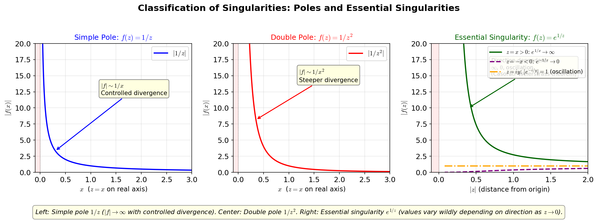
Fig. E.6: Classification of poles and essential singularities. Figure E_6: Left: Simple pole \(1/z\) (\(|f| \to \infty\) in a controlled divergence). Center: Second-order pole \(1/z^2\). Right: Essential singularity \(e^{1/z}\) (values oscillate wildly as \(z \to 0\)).

Relation to Mode Expansion

🟡 Lina: In the string quantization of Ch. 14, the field \(X^\mu(\sigma, \tau)\) was mode-expanded (see Ch. 14):

\[X^\mu = x^\mu + \alpha' p^\mu \ln|z|^2 + i\sqrt{\frac{\alpha'}{2}} \sum_{n \neq 0} \frac{\alpha_n^\mu}{n} z^{-n} + \cdots\]

This is essentially a Laurent expansion. Each mode \(\alpha_n^\mu\) corresponds to a Laurent coefficient \(a_n\).

🔵 Kai: Ah, the string mode expansion is a Laurent expansion itself. The \(\alpha_n\) are exactly the \(a_n\).

🟡 Lina: Exactly. In the conformal field theory of Ch. 16, the Laurent expansion coefficients of fields become mode operators, and their commutation relations determine the algebraic structure.

📝 Exercises:

• Laurent expansion and classification of singularities → Problem B-8. Laurent Expansion and Residue of \(1/z^2\), Problem B-9. Laurent Expansion of \(e^{1/z}\)

✅ Comprehension Check: In a Laurent expansion, what is the term with \(n < 0\) (negative power part) called?

Answer

It is called the principal part. It describes the structure of the singularity.

✅ Comprehension Check: What conditions on the Laurent expansion coefficients define \(z = z_0\) as a pole of order \(N\)?

Answer

\(a_{-N} \neq 0\) and \(a_n = 0\) for all \(n < -N\) (the principal part terminates at the \((z-z_0)^{-N}\) term).

✅ Comprehension Check: What is the relationship between string theory mode expansions and Laurent expansions?

Answer

Each coefficient of the field's Laurent expansion corresponds to a mode operator \(\alpha_n^\mu\).

---

E.7　Cauchy's Integral Formula and the Residue Theorem

Cauchy's Integral Theorem (Starting Point)

🟡 Lina: Let's start with the fundamental theorem. If \(f(z)\) is holomorphic inside a closed curve \(C\):

\[\oint_C f(z) \, dz = 0 \tag{E.14}\]

🔵 Kai: Why does the integral become 0 when the function is holomorphic?

🟡 Lina: Let me give an intuitive explanation. Decomposing the complex integral into real and imaginary parts:

\[\oint_C f(z)\,dz = \oint_C (u + iv)(dx + i\,dy) = \oint_C (u\,dx - v\,dy) + i\oint_C (v\,dx + u\,dy)\]

Using Green's theorem (the 2-dimensional Stokes' theorem) learned in General Relativity General Relativity Appendix A:

\[\oint_C (P\,dx + Q\,dy) = \iint_D \left(\frac{\partial Q}{\partial x} - \frac{\partial P}{\partial y}\right) dx\,dy\]

This theorem states the relation "line integral along a closed curve (left side) = area integral over the interior (right side)."

The left side is a line integral along the closed curve \(C\). Just like calculating "the work done by force \(\vec{F}\) on an object along a path \(W = \int \vec{F} \cdot d\vec{s}\)" in high school physics, \(\oint_C (P\,dx + Q\,dy)\) is the operation of "summing \(P \cdot dx + Q \cdot dy\) at each point on the curve."

The right side is an area integral over the region \(D\) enclosed by \(C\). The physical meaning of Green's theorem is: "the line integral along a closed curve (left side) = the sum of all small contributions in the interior (right side)." In a water flow analogy, the strength of flow going around the perimeter equals the sum of all vortices inside. (Intuitively, dividing \(D\) into small rectangles, contributions from adjacent shared edges cancel, leaving only the outer perimeter. See General Relativity General Relativity Appendix A for the rigorous proof.)

⚪ Mei: "Adjacent edges cancel" means that the shared edge between neighboring small squares is traversed in opposite directions, so they cancel. Only the outer boundary edges remain.

🟡 Lina: Exactly. Now let's prove Cauchy's integral theorem using Green's theorem. Applying to the real part integral (\(P = u\), \(Q = -v\)):

\[\oint_C (u\,dx - v\,dy) = \oint_C (P\,dx + Q\,dy) = \iint_D \left(\frac{\partial Q}{\partial x} - \frac{\partial P}{\partial y}\right) dx\,dy = \iint_D \left(-\frac{\partial v}{\partial x} - \frac{\partial u}{\partial y}\right) dx\,dy\]

By the Cauchy-Riemann condition \(\frac{\partial u}{\partial y} = -\frac{\partial v}{\partial x}\):

\[= \iint_D \left(-\frac{\partial v}{\partial x} + \frac{\partial v}{\partial x}\right) dx\,dy = 0\]

The imaginary part is similarly 0. Therefore \(\oint_C f(z)\,dz = 0\).

🔵 Kai: I see... for non-holomorphic functions, Cauchy-Riemann doesn't hold, so this cancellation doesn't happen and the integral isn't zero.

🟡 Lina: Exactly. The Cauchy-Riemann conditions enable the cancellation—this is the privilege of holomorphic functions.

Derivation of Cauchy's Integral Formula

🟡 Lina: Next, when \(f(z)\) is holomorphic inside \(C\) and \(z\) is a point inside \(C\):

\[\boxed{f(z) = \frac{1}{2\pi i} \oint_C \frac{f(w)}{w - z} \, dw} \tag{E.15}\]

Let me derive this.

The integrand \(g(w) = \frac{f(w)}{w-z}\) has a first-order pole at \(w = z\). Take a small circle \(C_\epsilon\) (radius \(\epsilon\)) centered at \(z\) inside \(C\).

\(g(w)\) is holomorphic in the region between \(C\) and \(C_\epsilon\) (since we've excluded \(w = z\)).

Let me explain the application of Cauchy's integral theorem to the annular region. Cauchy's integral theorem states "the integral along the boundary of a holomorphic region is 0." The boundary of the annular region consists of two curves—the outer \(C\) and the inner \(C_\epsilon\). However, the correct orientation for the "boundary" is the direction that keeps the region on the left. The outer \(C\) is counterclockwise, and the inner \(C_\epsilon\) is clockwise. If we standardize \(C_\epsilon\) to counterclockwise, the sign flips, so Cauchy's integral theorem gives:

\[\oint_C g(w)\,dw - \oint_{C_\epsilon} g(w)\,dw = 0\]

(Here \(\oint_{C_\epsilon}\) is counterclockwise.)

Therefore:

\[\oint_C \frac{f(w)}{w-z}\,dw = \oint_{C_\epsilon} \frac{f(w)}{w-z}\,dw\]

🔵 Kai: The integral on the outer curve equals the integral on the small inner circle. By "avoiding" the singularity to create an annular region where the function is holomorphic, we can use the integral theorem.

🟡 Lina: Exactly. Parametrize on \(C_\epsilon\) as \(w = z + \epsilon e^{i\theta}\) (\(0 \leq \theta \leq 2\pi\)), so \(dw = i\epsilon e^{i\theta} d\theta\), \(w - z = \epsilon e^{i\theta}\):

\[\oint_{C_\epsilon} \frac{f(w)}{w-z}\,dw = \int_0^{2\pi} \frac{f(z + \epsilon e^{i\theta})}{\epsilon e^{i\theta}} \cdot i\epsilon e^{i\theta}\,d\theta = i\int_0^{2\pi} f(z + \epsilon e^{i\theta})\,d\theta\]

Taking the limit \(\epsilon \to 0\), by continuity of \(f\), \(f(z + \epsilon e^{i\theta}) \to f(z)\):

\[= i \int_0^{2\pi} f(z)\,d\theta = 2\pi i \, f(z)\]

Therefore:

\[\oint_C \frac{f(w)}{w-z}\,dw = 2\pi i \, f(z)\]

Dividing both sides by \(2\pi i\) gives equation (E.15).

🔵 Kai: Amazing. The value of a holomorphic function is completely determined by its values on the boundary alone? For a smooth real function, you could have the same values on a circle but change them freely inside, so why doesn't that work for complex functions?

🟡 Lina: Good question. Real functions only require "smoothness," but holomorphic functions have the additional constraint of the Cauchy-Riemann conditions. This constraint is very strong and greatly restricts the function's degrees of freedom. This is the "rigidity" of holomorphic functions. Internal values are uniquely determined by boundary data. In physics, this is the foundation of analytic continuation of scattering amplitudes and dispersion relations.

Formula for Higher-Order Derivatives

🟡 Lina: Differentiating Cauchy's integral formula with respect to \(z\) gives the formula for the \(n\)-th derivative:

\[f^{(n)}(z) = \frac{n!}{2\pi i} \oint_C \frac{f(w)}{(w-z)^{n+1}}\,dw \tag{E.16}\]

This is obtained by differentiating both sides of equation (E.15) \(n\) times with respect to \(z\) (\(\partial/\partial z\) can be moved inside the \(\oint\)):

\[\frac{\partial}{\partial z} \frac{1}{w-z} = \frac{1}{(w-z)^2}, \quad \frac{\partial^2}{\partial z^2} \frac{1}{w-z} = \frac{2}{(w-z)^3}, \quad \ldots\]

In general, \(\frac{\partial^n}{\partial z^n} \frac{1}{w-z} = \frac{n!}{(w-z)^{n+1}}\).

Definition of Residue

🟡 Lina: The coefficient of \((z-z_0)^{-1}\) in the Laurent expansion is called the residue:

\[\text{Res}_{z=z_0} f(z) = a_{-1} \tag{E.17}\]

Setting \(n = -1\) in equation (E.13):

\[a_{-1} = \frac{1}{2\pi i} \oint_C f(w)\,dw\]

That is:

\[\oint_C f(z)\,dz = 2\pi i \, a_{-1} = 2\pi i \, \text{Res}_{z=z_0} f(z) \tag{E.18}\]

(\(C\) is a small circle enclosing only \(z_0\))

🔵 Kai: Out of all the terms in the Laurent expansion, only the \((z-z_0)^{-1}\) term contributes to the contour integral! This connects to the orthogonality calculation earlier where only \(k = -1\) survived.

Derivation of the Residue Theorem

🟡 Lina: Consider the case where there are multiple singularities \(z_1, z_2, \ldots, z_N\) inside the closed curve \(C\). Look at the situation in Fig. E.7 "Geometric meaning of the residue theorem" where each singularity is enclosed by a small circle.

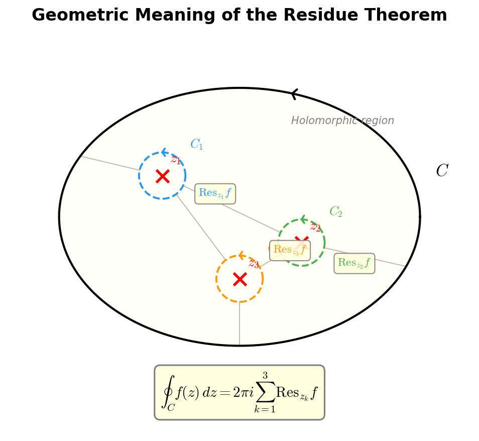
Fig. E.7: Geometric meaning of the residue theorem. Figure E_7: Each singularity \(z_k\) inside the closed curve \(C\) is enclosed by a small circle \(C_k\). The integral on \(C\) equals the sum of integrals on each \(C_k\) (= \(2\pi i \times\) residue).

Take small circles \(C_k\) enclosing each singularity \(z_k\). \(f\) is holomorphic in the region inside \(C\) with all \(C_k\) interiors removed. Applying Cauchy's integral theorem to this region:

\[\oint_C f(z)\,dz - \sum_{k=1}^{N} \oint_{C_k} f(z)\,dz = 0\]

By equation (E.18), each \(\oint_{C_k} f(z)\,dz = 2\pi i \, \text{Res}_{z=z_k} f(z)\), so:

\[\boxed{\oint_C f(z)\,dz = 2\pi i \sum_{k=1}^{N} \text{Res}_{z=z_k} f(z)} \tag{E.19}\]

This is the residue theorem.

⚪ Mei: So even without knowing the overall behavior of the integrand, the contour integral is completely determined by information near the singularities (residues) alone.

Methods for Computing Residues

🟡 Lina: Let me summarize the methods for actually computing residues.

For a simple pole: When \(f(z)\) has a first-order pole at \(z = z_0\):

\[\text{Res}_{z=z_0} f(z) = \lim_{z \to z_0} (z - z_0) f(z) \tag{E.20}\]

Derivation: Since \(f(z) = \frac{a_{-1}}{z-z_0} + a_0 + a_1(z-z_0) + \cdots\), we get \((z-z_0)f(z) = a_{-1} + a_0(z-z_0) + \cdots\). As \(z \to z_0\), \(a_{-1}\) remains.

For a pole of order \(N\): When \(f(z)\) has a pole of order \(N\) at \(z = z_0\):

\[\text{Res}_{z=z_0} f(z) = \frac{1}{(N-1)!} \lim_{z \to z_0} \frac{d^{N-1}}{dz^{N-1}} \left[(z-z_0)^N f(z)\right] \tag{E.21}\]

Derivation: \((z-z_0)^N f(z) = a_{-N} + a_{-N+1}(z-z_0) + \cdots + a_{-1}(z-z_0)^{N-1} + \cdots\)

Differentiating \((N-1)\) times, the \((z-z_0)^{N-1}\) term gives \((N-1)! \, a_{-1}\).

When \(f(z) = p(z)/q(z)\) and \(q\) has a simple zero:

\[\text{Res}_{z=z_0} \frac{p(z)}{q(z)} = \frac{p(z_0)}{q'(z_0)} \tag{E.22}\]

Derivation: \(q(z) \approx q'(z_0)(z-z_0)\) (\(z \to z_0\)), so \((z-z_0)f(z) \approx \frac{p(z_0)(z-z_0)}{q'(z_0)(z-z_0)} = \frac{p(z_0)}{q'(z_0)}\).

Calculation Examples

Example 1: Residue of \(f(z) = \frac{1}{z(z-1)}\) at \(z = 0\).

\(z = 0\) is a simple pole. Using equation (E.20):

\[\text{Res}_{z=0} \frac{1}{z(z-1)} = \lim_{z \to 0} z \cdot \frac{1}{z(z-1)} = \lim_{z \to 0} \frac{1}{z-1} = \frac{1}{-1} = -1\]

Example 2: Residue of \(f(z) = \frac{1}{z(z-1)}\) at \(z = 1\).

\[\text{Res}_{z=1} \frac{1}{z(z-1)} = \lim_{z \to 1} (z-1) \cdot \frac{1}{z(z-1)} = \lim_{z \to 1} \frac{1}{z} = 1\]

Example 3: Compute \(\oint_{|z|=2} \frac{1}{z(z-1)} dz\).

Both \(z = 0\) and \(z = 1\) are inside \(|z| = 2\). By the residue theorem:

\[\oint_{|z|=2} \frac{dz}{z(z-1)} = 2\pi i \left[\text{Res}_{z=0} + \text{Res}_{z=1}\right] = 2\pi i(-1 + 1) = 0\]

🔵 Kai: Oh, the residues \(-1\) and \(+1\) cancel out to give 0!

Example 4: Residue of \(f(z) = \frac{e^z}{z^2}\) at \(z = 0\).

\(z = 0\) is a second-order pole. Using equation (E.21) with \(N = 2\):

\[\text{Res}_{z=0} = \frac{1}{1!} \lim_{z \to 0} \frac{d}{dz}\left[z^2 \cdot \frac{e^z}{z^2}\right] = \lim_{z \to 0} \frac{d}{dz} e^z = \lim_{z \to 0} e^z = 1\]

Alternative: Since \(e^z = 1 + z + \frac{z^2}{2!} + \cdots\), we get \(\frac{e^z}{z^2} = \frac{1}{z^2} + \frac{1}{z} + \frac{1}{2} + \cdots\). So \(a_{-1} = 1\).

⚪ Mei: It's reassuring that both methods give the same answer. Reading the Laurent expansion directly might actually be more reliable.

📝 Exercises:

• Residue calculations → Problem B-7. Residue of \(1/(z-1)\), Problem M-2. Residues of \(z/[(z-1)(z-2)]\)
• Contour integral using the residue theorem → Problem M-1. Residue Theorem: Two Poles

The Power of the Residue Theorem — Applications to Real Integrals

🔵 Kai: Is the residue theorem only used for complex integrals?

🟡 Lina: Actually, it can be used for real integrals too. Here's a famous example.

\[I = \int_{-\infty}^{\infty} \frac{dx}{1 + x^2}\]

\(f(z) = \frac{1}{1+z^2} = \frac{1}{(z+i)(z-i)}\) has simple poles at \(z = \pm i\).

Take a large semicircular contour \(C_R\) in the upper half-plane (real axis \([-R, R]\) + semicircular arc of radius \(R\)) as the integration path (Fig. E.8 "Integration contour for real integrals using the residue theorem").

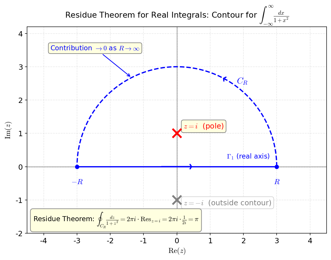
Fig. E.8: Integration contour for real integrals using the residue theorem. Figure E_8: Integration contour for computing \(\int_{-\infty}^{\infty} \frac{dx}{1+x^2}\): a closed curve combining the real axis \([-R, R]\) with a semicircular arc in the upper half-plane. Only the pole \(z = i\) in the upper half-plane contributes.

As \(R \to \infty\), the integral on the semicircular arc goes to 0 (\(|f| \sim 1/R^2\) and arc length \(\pi R\), so \(\sim \pi/R \to 0\)).

The only pole in the upper half-plane is \(z = i\):

\[\text{Res}_{z=i} \frac{1}{(z+i)(z-i)} = \lim_{z \to i} (z-i) \cdot \frac{1}{(z+i)(z-i)} = \frac{1}{2i}\]

By the residue theorem:

\[I = 2\pi i \cdot \frac{1}{2i} = \pi\]

⚪ Mei: The change of \(\arctan x\) from \(-\infty\) to \(\infty\) is \(\pi\), so it checks out!

Usage in Conformal Field Theory

🟡 Lina: In the OPE (operator product expansion) of Ch. 16, the singular behavior when two operators approach each other is described by a Laurent expansion:

\[A(z) B(w) \sim \sum_{n=1}^{N} \frac{C_n(w)}{(z - w)^n} + (\text{regular terms})\]

In particular, the coefficient of \((z-w)^{-1}\) (the residue) corresponds to commutation relations. The relation to mode expansions is:

\[A(z) = \sum_n A_n z^{-n-h_A}\]

(\(h_A\) is the conformal dimension of \(A\)). To extract the mode \(A_n\), use a contour integral:

\[A_n = \oint \frac{dz}{2\pi i} z^{n+h_A-1} A(z)\]

This is exactly the Laurent coefficient formula (E.13).

🔵 Kai: So extracting modes is done by contour integration. The Laurent coefficient formula directly connects to physics.

🟡 Lina: Furthermore, the commutation relation between modes of two operators is:

\[[A_m, B_n] = \oint_0 \frac{dw}{2\pi i} w^{n+h_B-1} \oint_w \frac{dz}{2\pi i} z^{m+h_A-1} A(z)B(w)\]

Here \(\oint_w\) is a contour integral encircling \(w\). Substituting the OPE and applying the residue theorem computes the commutation relations. This is the heart of the Virasoro algebra derivation in Ch. 16.

✅ Comprehension Check: The residue is which coefficient of the Laurent expansion?

Answer

The coefficient \(a_{-1}\) of \((z - z_0)^{-1}\).

✅ Comprehension Check: Why is the residue theorem formula \(\oint_C f(z)\,dz = 2\pi i \sum_k \text{Res}_{z=z_k} f(z)\) called a "remarkable property"?

Answer

Because the contour integral can be computed from information near the singularities (residues) alone, without knowing the overall behavior of the integrand.

✅ Comprehension Check: What does Cauchy's integral formula \(f(z) = \frac{1}{2\pi i}\oint_C \frac{f(w)}{w-z}dw\) mean physically?

Answer

The interior values of a holomorphic function are completely determined by boundary data alone (rigidity of holomorphic functions).

---

E.8　Green's Function for the 2D Free Field

🟡 Lina: At the beginning of Ch. 16 16.4 "Operator Product Expansion (OPE)", the two-point function of the free boson \(\langle X(z,\bar{z})\, X(w,\bar{w})\rangle = -\frac{\alpha'}{2}\ln\lvert z-w\rvert^2\) appeared without derivation. Here, we'll derive why this expression becomes a logarithmic function using only the tools prepared in E.3 "Complex Coordinates \(z, \bar{z}\) and Differentiation" and E.7 "Cauchy's Integral Formula and the Residue Theorem". We won't go into the details of path integrals, but once we reduce it to the fact that "the fundamental Green's function of the 2D Laplacian is logarithmic," the rest follows by calculation.

E.8.1　Free Field Action and Green's Function Equation

🟡 Lina: The action for the 2-dimensional free boson \(X(z, \bar{z})\) from Ch. 13 is:

\[ S = \frac{1}{2\pi\alpha'}\int d^2z\; \partial X\, \bar\partial X \]

Here we've suppressed the spacetime index \(\mu\) and written just one component. Extension to \(D\) fields \(X^\mu\) is done in "E.8.5　Extension to \(D\) Fields".

Here \(d^2z\) is a symbol for the area element (the superscript 2 means "2-dimensional," not "\(dz\) squared"), and in this appendix we define \(d^2z \equiv dx\,dy\). As shown in equation (E.7) of E.3 "Complex Coordinates \(z, \bar{z}\) and Differentiation", in complex coordinates this is \(d^2z = dx\,dy = \frac{i}{2}dz \wedge d\bar{z}\). That is, \(d^2z\) is simply the ordinary real-coordinate area element \(dx\,dy\).

(⚠️ Note: Some textbooks (e.g., Polchinski) define the area element as \(d^2z_{\text{Pol}} = 2dx\,dy\). In that case, the coefficient in front of the action changes, but the physical content is the same. When reading other references, check the definition of the area element.)

Also, we abbreviate \(\partial \equiv \partial_z\), \(\bar\partial \equiv \partial_{\bar{z}}\). The classical equation of motion is \(\partial \bar\partial X = 0\) (from E.3 "Complex Coordinates \(z, \bar{z}\) and Differentiation", since \(\nabla^2 = 4\partial\bar\partial\), this is the same as \(\nabla^2 X = 0\)).

🔵 Kai: I see, the equation of motion is the Laplace equation itself. This connects to what you said earlier about the solution separating into \(f(z) + g(\bar{z})\).

🟡 Lina: In quantum theory, the two-point function \(G(z, w) = \langle X(z,\bar{z})\, X(w,\bar{w})\rangle\) computed via the path integral satisfies the following equation. Let me identify the differential operator that determines the form of the equation from the variation of the action. First, let's check the coefficient of the differential operator. Varying the action \(S = \frac{1}{2\pi\alpha'}\int d^2z\, \partial X\, \bar\partial X\) with respect to \(X\). Taking the first variation under \(X \to X + \delta X\) gives \(\delta S = \frac{1}{2\pi\alpha'}\int d^2z\,(\partial(\delta X)\,\bar\partial X + \partial X\,\bar\partial(\delta X))\). Integrate each term by parts. Recall integration by parts in one dimension: \(\int_a^b u\,v'\,dx = [uv]_a^b - \int_a^b u'\,v\,dx\). The same can be done for area integrals in two dimensions—fixing \(\bar{z}\) and looking only in the \(z\) direction is the same as one-dimensional integration by parts.

🔵 Kai: So you're "pushing" the \(\partial\) in \(\partial(\delta X)\) onto the neighboring \(\bar\partial X\)? Like in one dimension where \(\int u'v\,dx = -\int uv'\,dx\) (ignoring boundary terms).

🟡 Lina: Exactly. In the first term \(\int d^2z\, (\partial(\delta X))\, \bar\partial X\), we move \(\partial\) by integration by parts from the \(\delta X\) side to the \(\bar\partial X\) side. The sign flips:

\[\int d^2z\, (\partial(\delta X))\, \bar\partial X = -\int d^2z\, \delta X\, \partial\bar\partial X + (\text{boundary terms})\]

Here we consider an infinitely large plane and assume \(X\) decays sufficiently fast at infinity, so boundary terms vanish (for a closed worldsheet, there's no boundary so they similarly vanish). In the second term \(\int d^2z\, \partial X\, (\bar\partial(\delta X))\), we now move \(\bar\partial\) from the \(\delta X\) side to the \(\partial X\) side. Integrating by parts in the same way gives a sign flip, yielding \(-\int d^2z\, (\bar\partial\partial X)\, \delta X\) (\(\bar\partial\) acts on \(\partial X\) to give \(\bar\partial\partial X\)). Since \(\partial\bar\partial = \bar\partial\partial\) (interchange of mixed partial derivatives) holds, both terms become \(-\frac{1}{2\pi\alpha'}\int d^2z\,(\partial\bar\partial X)\,\delta X\), and combining gives:

\[\delta S = -\frac{1}{\pi\alpha'}\int d^2z\,(\partial\bar\partial X)\,\delta X\]

⚪ Mei: I see, the first term gives \(\partial\bar\partial X\) and the second term gives the same thing, so the coefficient doubles and \(1/(2\pi\alpha')\) becomes \(1/(\pi\alpha')\).

🟡 Lina: Right. Since \(\delta S = 0\) must hold for arbitrary \(\delta X\), the equation of motion \(-\frac{1}{\pi\alpha'}\partial\bar\partial X = 0\) is obtained. So the differential operator is \(-\frac{1}{\pi\alpha'}\partial\bar\partial\).

The Green's function is defined as the "inverse" of this differential operator:

\[ \boxed{-\frac{1}{\pi\alpha'}\partial_z\partial_{\bar{z}} G(z, w) = \delta^{(2)}(z-w)} \]

That is:

\[\partial_z\partial_{\bar{z}} G = -\pi\alpha'\, \delta^{(2)}(z-w) \qquad (\star)\]

Here \(\delta^{(2)}(z-w) = \delta(x-x')\delta(y-y')\) is normalized as \(\int d^2z\, \delta^{(2)}(z-w) = 1\) (\(d^2z = dx\,dy\), our convention). (In references using the Polchinski convention \(d^2z_{\text{Pol}} = 2dx\,dy\), the delta function normalization is also adjusted to \(\int d^2z_{\text{Pol}}\, \delta_{\text{Pol}}^{(2)} = 1\), so \(\delta_{\text{Pol}}^{(2)} = \frac{1}{2}\delta^{(2)}\), and the coefficient on the right side of the equation changes. The final form of the Green's function is the same.)

🔵 Kai: What's the \(\delta^{(2)}\) on the right? Classically it was \(\nabla^2 X = 0\), so why does a delta function appear on the right? And \(\delta^{(2)}\) isn't an ordinary function, right?

🟡 Lina: Good question. Let me first explain what \(\delta^{(2)}(z-w)\) is. This is the 2-dimensional version of the Dirac delta function, which in real coordinates is \(\delta(x-x')\delta(y-y')\). It's not an ordinary function but a "distribution" defined by the property \(\int d^2z\; \delta^{(2)}(z-w) f(z) = f(w)\). It's like a filter that "picks out the value only at point \(w\)."

🔵 Kai: "Picks out the value only at point \(w\)" — does that mean it's zero everywhere except \(z = w\)? But if you integrate a function that's zero, wouldn't you get zero?

🟡 Lina: That's where it differs from ordinary functions. The delta function has an "infinitely sharp peak at \(z = w\)" with zero width but infinite height, adjusted so that the area (integral value) is exactly 1. For example, think of a rectangle with width \(\epsilon\) and height \(1/\epsilon\). The area is always 1, but as \(\epsilon \to 0\) it becomes a "needle" with zero width and infinite height. This is the intuitive image of the delta function. Strictly speaking, it's not an ordinary function but a mathematical object called a "distribution" that only has meaning inside integrals.

🔵 Kai: I see, "a needle with area 1." Then why does it appear on the right side of the Green's function equation?

🟡 Lina: Think of it intuitively like this. The Green's function \(G(z, w)\) represents "the effect at point \(z\) of a point source placed at point \(w\)." It's the same structure as finding the potential of a point charge in electromagnetism, where the delta function of the point charge enters the right side of \(\nabla^2 \phi = -\rho/\epsilon_0\). In quantum theory, the two-point function plays the role of this "response function to a point source."

More concretely, the equation "\(\mathcal{O}\, G = \delta\)" (\(\mathcal{O}\) is a differential operator) means "applying \(\mathcal{O}\) to \(G\) returns a response concentrated only at point \(w\)." It has the same structure as solving the simultaneous equation \(Ax = b\) to get \(x = A^{-1}b\) from high school — \(\mathcal{O}\) is the "matrix \(A\)," \(G\) is the "inverse matrix \(A^{-1}\)," and \(\delta\) is the "identity matrix \(I\)." That is, \(A A^{-1} = I\) and \(\mathcal{O} G = \delta\) have the same structure — "multiplying the operator by its inverse gives the identity." The \(\delta^{(2)}\) on the right is derived from path integral techniques (see Quantum Field Theory Quantum Field Theory Ch. 11 on generating functionals). Here, let's accept the rule "define the inverse of the differential operator \(\mathcal{O}\) by \(\mathcal{O}G = \delta\)" and proceed. It's exactly the same idea as finding a point charge potential from \(\nabla^2 \phi = -\rho/\varepsilon_0\) in electromagnetism — place a point source (delta function) on the right and find the response.

🔵 Kai: So \(G\) is "the inverse of a differential operator." But inverse matrices can be computed because matrices have finite size, right? A differential operator is like an "infinite-dimensional matrix" — is the existence of its inverse guaranteed?

🟡 Lina: Sharp question. In general, the inverse doesn't necessarily exist — without specifying boundary conditions, the solution may not be unique. Here, by imposing the condition "on an infinite plane, without diverging too much at infinity," the solution is determined uniquely (up to a constant ambiguity). I'll skip the rigorous existence proof, but since we'll actually construct the solution below, "does the inverse exist?" can be confirmed by "can we find the solution?"

Finding the solution to \((\star)\) — the "fundamental Green's function" of the 2D Laplacian — determines \(G\).

E.8.2　The Key Formula: \(\partial_{\bar{z}} (1/(z-w))\) is a Delta Function

🟡 Lina: The essential formula of this section is:

\[ \boxed{\partial_{\bar{z}}\, \frac{1}{z-w} = \pi\, \delta^{(2)}(z-w)} \qquad (\star\star) \]

It looks surprising at first, but I'll prove it below.

First, it's 0 for \(z \neq w\):

For \(z \neq w\), \(1/(z-w)\) is a holomorphic function of \(z\). As seen in E.4 "Holomorphic Functions and the Cauchy-Riemann Conditions", holomorphic functions are annihilated by \(\partial_{\bar{z}}\):

\[ \partial_{\bar{z}}\, \frac{1}{z-w} = 0 \qquad (z \neq w) \]

So the left side has a contribution concentrated only at the "singularity" \(z = w\). Recall the properties of the \(\delta\) function explained earlier — "zero for \(z \neq w\) but returns a finite value when integrated over a region containing \(z = w\)." The only object satisfying both properties simultaneously is the \(\delta\) function (being zero for \(z \neq w\) yet having a finite integral — impossible for ordinary functions, but exactly the behavior of \(\delta\) functions). Below we'll actually integrate and confirm that the finite value is \(\pi\). So \(\partial_{\bar{z}}(1/(z-w)) = (\text{constant}) \times \delta^{(2)}(z-w)\) is already established, and we just need to determine the constant.

🔵 Kai: I see, it's zero for \(z \neq w\) but integrating doesn't give zero — that's exactly the characteristic of a delta function. We just need to verify the coefficient.

🟡 Lina: Next, let's confirm that integrating near \(z = w\) gives a non-zero value.

Integrate the left side of \((\star\star)\) over a small disk \(D\) (radius \(\epsilon\)) centered at \(z = w\). If the result is \(\pi\), then \((\star\star)\) is correct (since \(\int d^2z\; \pi\delta^{(2)}(z-w) = \pi\)).

What we need here is Green's theorem in complex coordinates. This is just Green's theorem \(\oint(P\,dx + Q\,dy) = \iint_D(\partial_x Q - \partial_y P)\,dx\,dy\) used in E.7 "Cauchy's Integral Formula and the Residue Theorem" to derive Cauchy's integral theorem, rewritten in complex coordinates \((z, \bar{z})\). The result is:

\[ \int_D d^2z\; \partial_{\bar{z}} f(z, \bar{z}) = \frac{1}{2i}\oint_{\partial D} f\, dz \]

🔵 Kai: Where does the \(\frac{1}{2i}\) come from?

🟡 Lina: Let's derive it. Using Green's theorem is most direct.

Since \(dz = dx + i\,dy\), we have \(f\,dz = f(dx + i\,dy) = f\,dx + (if)\,dy\). Comparing with Green's theorem \(\oint_{\partial D}(P\,dx + Q\,dy) = \iint_D (\partial_x Q - \partial_y P)\, dx\, dy\), we read off \(P = f\), \(Q = if\). Therefore:

\[\oint_{\partial D} f\, dz = \iint_D \left(\frac{\partial(if)}{\partial x} - \frac{\partial f}{\partial y}\right) dx\, dy = \iint_D \left(i\frac{\partial f}{\partial x} - \frac{\partial f}{\partial y}\right) dx\, dy\]

Let me rewrite \(i\partial_x f - \partial_y f\) in terms of \(\partial_{\bar{z}}\). From equation (E.4), \(\partial_{\bar{z}} = \frac{1}{2}(\partial_x + i\partial_y)\), so \(2i\partial_{\bar{z}} = i(\partial_x + i\partial_y) = i\partial_x + i^2\partial_y = i\partial_x - \partial_y\).

⚪ Mei: I see, using \(2i\partial_{\bar{z}} = i\partial_x - \partial_y\) that Lina just showed, the integrand neatly becomes \(2i\partial_{\bar{z}} f\).

🟡 Lina: Exactly. Using this:

\[\oint_{\partial D} f\, dz = \iint_D 2i\, \partial_{\bar{z}} f\; dx\, dy = 2i \int_D \partial_{\bar{z}} f\, d^2z\]

Dividing both sides by \(2i\):

\[\int_D d^2z\; \partial_{\bar{z}} f = \frac{1}{2i}\oint_{\partial D} f\, dz\]

🔵 Kai: I see, the \(\frac{1}{2i}\) is the coefficient that comes from rewriting the right side of Green's theorem in terms of \(\partial_{\bar{z}}\).

Substituting \(f = 1/(z-w)\):

Take \(\partial D\) as a circle of radius \(\epsilon\) centered at \(w\). Note: \(1/(z-w)\) is singular at \(z = w\), but the region \(D\) to which we apply Green's theorem is "the disk of radius \(\epsilon\) centered at \(w\)," and on its boundary \(\partial D\), \(|z - w| = \epsilon \neq 0\), so \(f\) is smooth. The singularity at \(z = w\) in the interior is precisely what this integral "detects" — the left-side area integral picks up the contribution from \(z = w\).

\[ \int_D dx\,dy\; \partial_{\bar{z}}\frac{1}{z-w} = \frac{1}{2i}\oint_{\lvert z-w\rvert=\epsilon} \frac{dz}{z-w} \]

The right side is the fundamental form of Cauchy's integral formula computed in E.7 "Cauchy's Integral Formula and the Residue Theorem":

\[ \oint_{\lvert z-w\rvert=\epsilon} \frac{dz}{z-w} = 2\pi i \]

Therefore:

\[ \int_D dx\,dy\; \partial_{\bar{z}}\frac{1}{z-w} = \frac{1}{2i}\cdot 2\pi i = \pi \]

The result remains \(\pi\) no matter how small \(\epsilon\) is. Meanwhile, the integrand is zero for \(z \neq w\). So we have "a singularity of strength \(\pi\) concentrated at \(z = w\)" = "\(\pi\, \delta^{(2)}(z-w)\)."

This proves formula \((\star\star)\):

\[ \partial_{\bar{z}}\, \frac{1}{z-w} = \pi\, \delta^{(2)}(z-w) \]

⚪ Mei: Cauchy's integral formula reappears here beautifully. The tools prepared in §E.7 fit perfectly.

🟡 Lina: By the way, this has essentially the same structure as the 3-dimensional formula \(\nabla^2 (1/r) = -4\pi\delta^{(3)}(\vec{r})\) seen in General Relativity General Relativity Appendix A. That was the Green's function of the 3D Laplacian being \(1/r\), and here it's the 2D version.

🔵 Kai: Ah, it's the same structure as the point charge potential story! Just different dimensions.

E.8.3　Derivation of the Logarithmic Green's Function

🟡 Lina: Let me construct the solution to \((\star)\) using \((\star\star)\).

Formula \((\star\star)\) shows that "applying \(\partial_{\bar{z}}\) to \(1/(z-w)\) produces a delta function." That is, \(1/(z-w)\) is the function that "unwinds one level" of the inverse of \(\partial_{\bar{z}}\). If we unwind one more level for \(\partial_z\) too, the Green's function is complete. So:

🔵 Kai: "Unwinding one more level" means finding the original function whose \(z\)-derivative gives \(1/(z-w)\)? In real numbers, \(\frac{d}{dx}\ln x = 1/x\), so \(\ln(z-w)\) seems like a candidate... does it work for complex numbers too?

🟡 Lina: Exactly! Just as \(\int \frac{1}{x}\,dx = \ln x\) for real numbers, \(\partial_z \ln(z-w) = 1/(z-w)\) holds. More precisely, think of it as "finding the function whose derivative gives \(1/(z-w)\)" rather than "integrating."

🔵 Kai: Does differentiating the complex logarithm also give \(1/z\)? Same as the real case?

🟡 Lina: Let's verify. The most direct method: differentiating both sides of \(e^{\ln z} = z\) with respect to \(z\) gives \(e^{\ln z} \cdot \frac{d(\ln z)}{dz} = 1\). Since \(e^{\ln z} = z\), we get \(\frac{d(\ln z)}{dz} = 1/z\) ✓.

(Alternative verification: writing \(\ln z = \ln r + i\theta\) and computing \(\partial_z\) also gives \(1/z\). You can confirm using \(\partial_z \bar{z} = 0\), so try it as a practice problem if interested.)

However, extending \(\ln z\) to complex numbers requires some care. The argument \(\theta\) has freedom up to integer multiples of \(2\pi\) (\(e^{i\theta} = e^{i(\theta + 2\pi)}\)), so \(\ln z\) can take infinitely many values for a single \(z\) — this is called a "multi-valued function." In practice, we choose a range for the argument (e.g., \(-\pi < \theta \leq \pi\)) to select one value. This choice is called "choosing a branch." Regardless of which branch we choose, differentiating gives \(\frac{d}{dz}\ln z = 1/z\), and the following calculations are unaffected. Therefore:

\[ \partial_z\partial_{\bar{z}} \ln(z-w) = \partial_{\bar{z}}\, \frac{1}{z-w} = \pi\, \delta^{(2)}(z-w) \qquad (\star\star\star) \]

That is, \(\partial_z \ln(z-w) = 1/(z-w)\) "unwinds" the first differentiation, and \(\partial_{\bar{z}}(1/(z-w)) = \pi\delta^{(2)}\) "unwinds" the second differentiation. We're constructing the inverse of \(\partial_z\partial_{\bar{z}}\) — the Green's function — in two stages.

🔵 Kai: Using two formulas in sequence to "unwind" the differential operator in two stages. But wait, \(\ln(z-w)\) is a function of \(z\) only, right? Where did the \(\bar{z}\) direction information go? Shouldn't it have both like \(\ln|z-w|^2\)?

🟡 Lina: Good observation. Actually, \(\ln\lvert z-w\rvert^2 = \ln(z-w) + \ln(\overline{z-w})\) is more symmetric and easier to work with. (This equality comes from \(|z-w|^2 = (z-w)(\overline{z-w})\) and the property \(\ln(AB) = \ln A + \ln B\). You might worry about the multi-valuedness of complex logarithms, but when taking partial derivatives \(\partial_z\) or \(\partial_{\bar{z}}\), the constant part from multi-valuedness disappears, so it doesn't affect the following calculations.) The second term similarly:

(Note that \(\partial_z\partial_{\bar{z}} = \partial_{\bar{z}}\partial_z\) always holds for smooth functions (interchange of mixed partial derivatives). The singularity at \(z = w\) was individually verified above as a delta function. Below we calculate in the order of applying \(\partial_{\bar{z}}\) first, then \(\partial_z\).)

Since \(\overline{z-w} = \bar{z} - \bar{w}\), \(\ln(\overline{z-w}) = \ln(\bar{z} - \bar{w})\) is a function of \(\bar{z}\) only (independent of \(z\), an anti-holomorphic function). First, apply the inner \(\partial_{\bar{z}}\). For a function \(g(\bar{z})\) of \(\bar{z}\) alone, \(\partial_{\bar{z}} g(\bar{z}) = \frac{dg}{d\bar{z}}\) holds (check: applying \(\partial_{\bar{z}} = \frac{1}{2}(\partial_x + i\partial_y)\) to \(g(\bar{z}) = g(x - iy)\), by the chain rule we get \(\frac{1}{2}(g' \cdot 1 + i \cdot g' \cdot (-i)) = \frac{1}{2}(g' + g') = g'\) ✓). Therefore \(\partial_{\bar{z}} \ln(\bar{z} - \bar{w}) = \frac{1}{\bar{z} - \bar{w}} = \frac{1}{\overline{z-w}}\).

Next, apply the outer \(\partial_z\). For \(z \neq w\), \(\frac{1}{\overline{z-w}}\) is a function of \(\bar{z}\) only, so it vanishes under \(\partial_z\), but at \(z = w\) it has a singularity and a delta function appears.

The intuition is this. Formula \((\star\star)\) said "\(1/(z-w)\) is a holomorphic function of \(z\) for \(z \neq w\), so \(\partial_{\bar{z}}\) kills it, but the singularity \(z = w\) is the exception and produces a delta function." Now it's "\(1/(\overline{z-w})\) is a function of \(\bar{z}\) only for \(z \neq w\), so \(\partial_z\) kills it, but the singularity \(z = w\) is the exception" — the same structure with the roles of \(z\) and \(\bar{z}\) exchanged. But saying "same structure therefore same result" isn't sufficient, so below we explicitly confirm using the \(\bar{z}\)-version of Stokes' theorem. The formula to show is:

\[ \partial_z\partial_{\bar{z}} \ln(\overline{z-w}) = \partial_z\, \frac{1}{\overline{z-w}} = \pi\, \delta^{(2)}(z-w) \]

⚪ Mei: So this is the "mirror version" calculation with \(z\) and \(\bar{z}\) roles swapped.

🟡 Lina: As with \((\star\star)\), we confirm by integrating over a small disk \(D\) (centered at \(w\), radius \(\epsilon\)). There's also a \(\bar{z}\)-version of the complex-coordinate Stokes' theorem:

\[\int_D d^2z\; \partial_z g = -\frac{1}{2i}\oint_{\partial D} g\, d\bar{z}\]

The derivation uses the same method as the \(z\)-version. Let's verify step by step. Since \(d\bar{z} = dx - i\,dy\), \(g\,d\bar{z} = g\,dx + (-ig)\,dy\). In Green's theorem \(\oint(P\,dx + Q\,dy) = \iint_D(\partial_x Q - \partial_y P)\,dx\,dy\), setting \(P = g\), \(Q = -ig\) gives the left side as \(\oint_{\partial D} g\,d\bar{z}\) ✓. The integrand on the right is:

\[\partial_x(-ig) - \partial_y(g) = -i\partial_x g - \partial_y g\]

From equation (E.3), \(\partial_z = \frac{1}{2}(\partial_x - i\partial_y)\), so \(-2i\partial_z = -2i \cdot \frac{1}{2}(\partial_x - i\partial_y) = -i\partial_x + i^2\partial_y = -i\partial_x - \partial_y\) ✓. Therefore:

\[\oint_{\partial D} g\,d\bar{z} = \iint_D (-2i\,\partial_z g)\,dx\,dy = -2i \int_D \partial_z g\, d^2z\]

Dividing both sides by \(-2i\):

\[\int_D d^2z\; \partial_z g = -\frac{1}{2i}\oint_{\partial D} g\, d\bar{z}\]

Substituting \(g = 1/\overline{z-w}\). Parametrize on \(\partial D\) as \(z = w + \epsilon e^{i\theta}\) (\(0 \leq \theta \leq 2\pi\), counterclockwise). Taking the complex conjugate: \(\bar{z} = \bar{w} + \epsilon e^{-i\theta}\), \(d\bar{z} = -i\epsilon e^{-i\theta}d\theta\), \(\overline{z-w} = \epsilon e^{-i\theta}\), so:

\[\oint_{\partial D} \frac{d\bar{z}}{\overline{z-w}} = \int_0^{2\pi}\frac{-i\epsilon e^{-i\theta}}{\epsilon e^{-i\theta}}d\theta = -2\pi i\]

Therefore \(\int_D d^2z\; \partial_z \frac{1}{\overline{z-w}} = -\frac{1}{2i}\cdot(-2\pi i) = \pi\), and the result is the same \(\pi\delta^{(2)}(z-w)\).

🔵 Kai: Both the \(z\)-version and the \(\bar{z}\)-version give the same \(\pi\). It's expected from symmetry, but it's reassuring to confirm by calculation.

🟡 Lina: Since \(\ln|z-w|^2 = \ln(z-w) + \ln(\overline{z-w})\), distributing \(\partial_z\partial_{\bar{z}}\) to each term and adding (differentiation is a linear operator so it distributes over sums):

\[ \partial_z\partial_{\bar{z}} \ln\lvert z-w\rvert^2 = \underbrace{\partial_z\partial_{\bar{z}} \ln(z-w)}_{= \pi\delta^{(2)}(z-w)} + \underbrace{\partial_z\partial_{\bar{z}} \ln(\overline{z-w})}_{= \pi\delta^{(2)}(z-w)} \]

\[ \boxed{\partial_z\partial_{\bar{z}} \ln\lvert z-w\rvert^2 = 2\pi\, \delta^{(2)}(z-w)} \]

E.8.4　Completing the Two-Point Function

🟡 Lina: Comparing the Green's function equation \((\star)\):

\[ \partial_z\partial_{\bar{z}} G(z,w) = -\pi\alpha'\, \delta^{(2)}(z-w) \]

with what we just derived:

\[ \partial_z\partial_{\bar{z}}\left[-\frac{\alpha'}{2}\ln\lvert z-w\rvert^2\right] = -\frac{\alpha'}{2}\cdot 2\pi\, \delta^{(2)}(z-w) = -\pi\alpha'\, \delta^{(2)}(z-w) \]

The two agree including coefficients. Therefore:

\[ \boxed{G(z, w) = \langle X(z,\bar{z})\, X(w,\bar{w})\rangle = -\frac{\alpha'}{2}\ln\lvert z-w\rvert^2} \]

🔵 Kai: There it is! The formula that was stated without proof in Ch. 16 is naturally derived just by inverting the Laplacian.

⚪ Mei: And the only tools used along the way were Euler's formula, the Cauchy-Riemann conditions, and Cauchy's integral formula — all things we prepared step by step in this appendix.

🔵 Kai: Comparing to the 3D formula \(\nabla^2(1/r) = -4\pi\delta^{(3)}\) I mentioned earlier, in 3D the Green's function is \(1/r\), and in 2D it's \(\ln r\). Why does the form change when the dimension changes?

🟡 Lina: Good comparison. In general, the Green's function of the \(d\)-dimensional Laplacian is \(r^{2-d}\) for \(d \geq 3\) and \(\ln r\) for \(d = 2\). This is determined by Gauss's law (the flux through a sphere is constant). The form of the Green's function changes with dimension, but the structure of "inverse of the Laplacian" is common. And this logarithmic Green's function is the starting point for all OPE calculations in Ch. 16.

E.8.5　Extension to \(D\) Fields

🟡 Lina: In string theory, there are \(D\) spacetime coordinates \(X^\mu\) (\(\mu = 0, 1, \ldots, D-1\)), each behaving as an independent free field. Since fields with different indices don't mix:

\[ \langle X^\mu(z)\, X^\nu(w)\rangle = -\frac{\alpha'}{2}\, \eta^{\mu\nu}\, \ln\lvert z-w\rvert^2 \]

Here \(\eta^{\mu\nu}\) is the Minkowski metric (General Relativity General Relativity Ch. 4). This is exactly the formula written "without proof" at the beginning of Ch. 16 16.4 "Operator Product Expansion (OPE)".

E.8.6　Direct Calculation of the \(\partial X\) OPE

🟡 Lina: What's actually used in Ch. 16 is the OPE between \(\partial X\) fields. Differentiating \(G(z,w) = -\frac{\alpha'}{2}\eta^{\mu\nu}\ln\lvert z-w\rvert^2\) with respect to \(z\) and \(w\) respectively. The order of differentiation and expectation value can be exchanged (differentiating the path integral integrand before integrating gives the same result as integrating then differentiating — this holds when conditions for interchanging integration and differentiation are met; we accept this here), so \(\partial_z \langle X^\mu(z)\, X^\nu(w)\rangle = \langle \partial X^\mu(z)\, X^\nu(w)\rangle\).

First with respect to \(z\):

\[ \langle \partial X^\mu(z)\, X^\nu(w)\rangle = \partial_z \langle X^\mu(z)\, X^\nu(w)\rangle = -\frac{\alpha'}{2}\eta^{\mu\nu}\, \partial_z \ln\lvert z-w\rvert^2 = -\frac{\alpha'}{2}\eta^{\mu\nu}\cdot \frac{1}{z-w} \]

(Of \(\ln\lvert z-w\rvert^2 = \ln(z-w) + \ln(\overline{z-w})\), for \(z \neq w\) the anti-holomorphic part \(\ln(\overline{z-w})\) vanishes under \(\partial_z\), so only the holomorphic part contributes. As seen in E.8.3, at \(z = w\) a delta-function contact term arises, but in OPE we focus on the singular structure for \(z \neq w\), so contact terms are ignored.)

Then with respect to \(w\):

\[ \partial_w\, \frac{1}{z-w} = \frac{1}{(z-w)^2} \]

Therefore:

\[ \boxed{\langle \partial X^\mu(z)\, \partial X^\nu(w)\rangle = -\frac{\alpha'}{2}\, \frac{\eta^{\mu\nu}}{(z-w)^2}} \]

This is the "fundamental contraction" for all OPE calculations in Ch. 16. Once derived, all that remains is counting combinations using Wick's theorem.

🔵 Kai: Differentiating the logarithm twice gives \(1/(z-w)^2\) — that's elegant. So this was the starting point of those OPEs.

📝 Exercises:

• Compute the cross term \(\langle \partial X^\mu(z)\, \bar\partial X^\nu(w)\rangle\) → Problem A-2. Cross Terms of \(\partial X\) and \(\bar\partial X\)

✅ Comprehension Check: Why does a delta function appear on the right side of the formula \(\partial_{\bar{z}}(1/(z-w)) = \pi\delta^{(2)}(z-w)\)?

Answer

For \(z \neq w\), \(1/(z-w)\) is a holomorphic function so \(\partial_{\bar{z}}\) kills it, but it has a singularity at \(z = w\). Integrating over a small disk gives a finite value \(\pi\) by Cauchy's integral formula, so the "singularity concentrated at \(z = w\)" is interpreted as a delta function.

✅ Comprehension Check: What is the physical/mathematical reason the free boson two-point function becomes a logarithmic function?

Answer

Because the fundamental Green's function of the 2D Laplacian is logarithmic. It has the same structure as the fundamental Green's function of the 3D Laplacian being \(1/r\) (Coulomb potential) — changing dimension changes the form to logarithmic.

✅ Comprehension Check: How is the singular part (coefficient of \((z-w)^{-2}\)) of the \(\partial X^\mu(z)\, \partial X^\nu(w)\) OPE expressed?

Answer

\(-\frac{\alpha'}{2}\,\eta^{\mu\nu}\). Differentiating the two-point function twice with respect to \(z, w\) differentiates the logarithm twice, giving the \(1/(z-w)^2\) form.

---

E.9　Practice Problems

📝 Exercises:

• Polar form and absolute value/argument of complex numbers → Problem B-1. Absolute Value and Argument of Complex Numbers
• Verification of Euler's formula → Problem B-2. Euler's Formula \(e^{i\pi}+1=0\)
• Product and quotient of complex numbers in polar form → Problem B-3. Product in Polar Form
• Verification of Cauchy-Riemann relations → Problem B-4. Cauchy-Riemann: Verification with \(z^2\)
• Identifying non-holomorphic functions → Problem B-5. Cauchy-Riemann: \(|z|^2\) Fails
• Verification of partial derivatives in complex coordinates → Problem B-6. \(\partial_z(z^2) = 2z\)
• Residue calculation (simple pole) → Problem B-7. Residue of \(1/(z-1)\)
• Laurent expansion and classification of singularities → Problem B-8. Laurent Expansion and Residue of \(1/z^2\)
• Contour integral using the residue theorem → Problem M-1. Residue Theorem: Two Poles
• Residue of higher-order poles → Problem M-2. Residues of \(z/[(z-1)(z-2)]\)
• Laurent expansion of an essential singularity → Problem B-9. Laurent Expansion of \(e^{1/z}\)
• Concrete example of conformal mapping (\(w = z^2\)) → Problem A-1. Conformal Mapping \(w = 1/z\)
• Composition of Möbius transformations → Problem M-3. Composition of Möbius Transformations
• Calculation of \(\partial X\) and \(\bar\partial X\) cross terms → Problem A-2. Cross Terms of \(\partial X\) and \(\bar\partial X\)

---

Preview of Next Chapter

In Appendix F, we survey the history of string theory in timeline format and compile an index of key figures from each era. By seeing at a glance "when and by whom" the models and concepts from the main text were proposed, the flow of physics development should become three-dimensional.

---

References

• David Tong, Lectures on String Theory, Ch.4: "Introducing Conformal Field Theory" — Conformal transformations in complex coordinates, OPE
• Elias Kiritsis, String Theory in a Nutshell, Ch.4: "Conformal Field Theory" — Physical applications of holomorphic functions and conformal maps
• Volker Schomerus, A Primer on String Theory, Ch.13: "Introduction to Conformal Field Theory" — Physical meaning of Laurent expansions and residues
• 杉浦光夫, 『解析入門 II』, 東京大学出版会 — Rigorous introduction to complex analysis
• Ahlfors, Complex Analysis, McGraw-Hill — Standard textbook on complex analysis

← D Group Theory and SymmetryF Timeline and Index of Key F… →

Feedback on this page

Let us know if something was unclear, incorrect, or could be improved.

Submit