Chapter 6: Curvilinear Coordinates and the Metric Tensor¶
Story so far: In Ch. 5, we derived the equivalence principle (Einstein's equivalence principle) from thought experiments involving a freely falling elevator and an accelerating rocket. Acceleration and gravity are locally indistinguishable—meaning gravity might not be a "force" but rather "a property of spacetime itself." If so, we need mathematical tools to describe "curved spacetime."
Goals of This Chapter
- Understand the mechanism of coordinate transformations (Jacobian matrix) and the meaning of the metric tensor \(g_{\mu\nu}\) through concrete examples of curvilinear coordinates (polar coordinates, spherical coordinates)
- Be able to express mathematically what it means for "the ruler to change from place to place," and furthermore distinguish that "curvature of coordinates" and "curvature of space" are separate concepts
- This forms the essential foundation for treating curved spacetime (Schwarzschild metric, etc.) in subsequent chapters
Unit system for this chapter: To make the correspondence with special relativity clear, we use SI units with \(c\) explicit. The 4-dimensional spacetime coordinates are \((t, x, y, z)\) (\(x^0 = t\)), which differs from the \((ct, x, y, z)\) used in previous chapters. See Appendix D.6 for conversion rules.
6.1 Why Cartesian Coordinates Alone Are Not Enough¶
🟡 Lina: In the previous chapter, we arrived at the idea that "gravity is the curvature of spacetime." But to describe "curved spacetime," we first need to become comfortable handling coordinates in "flat space."
🔵 Kai: Wait, if the space is flat, isn't ordinary \(x, y, z\) sufficient?
🟡 Lina: True, in flat space you can write everything in Cartesian coordinates. But there are many situations where you want to use different coordinates matched to the symmetry of the problem. For example, describing circular motion in \(x, y\) makes the equations complicated, but polar coordinates \((r, \theta)\) give much clearer expressions, right?
🟡 Lina: And there's an even more fundamental reason. In curved spacetime—for example, on a sphere—Cartesian coordinates that cover the entire space simply don't exist. Think about the surface of the Earth. It's impossible to cover the entire globe without distortion using flat \(x, y\) coordinates. That's why handling curvilinear coordinates is an essential tool for progressing to general relativity.
⚪ Mei: I see—you can tell just from looking at an atlas that a sphere can't be covered by flat coordinates. Every map projection inevitably introduces distortion.
🔵 Kai: I see... so first we practice "changing coordinates" in flat space, and then we move on to genuinely curved spaces.
🟡 Lina: Exactly. In this chapter, by introducing polar and spherical coordinates in flat space, we first understand the situation where the coordinates are curved but the space itself is not curved. Then we'll formalize "how to measure distance" in equations.
✅ Comprehension Check: Can you introduce Cartesian coordinates that cover an entire curved space (such as a sphere)?
Answer
No. On a curved space like a sphere, Cartesian coordinates that cover the entire surface without distortion do not exist. This is one of the fundamental reasons for learning to handle curvilinear coordinates.
✅ Comprehension Check: Are "curvature of coordinates" and "curvature of space" the same concept?
Answer
They are different concepts. Even in flat space, if you use curvilinear coordinates (such as polar coordinates), the coordinate lines are curved, but the space itself is not curved. It's important not to confuse the two.
6.2 Concrete Examples of Curvilinear Coordinates¶
Polar Coordinates (2 Dimensions)¶
🟡 Lina: The most familiar curvilinear coordinates are polar coordinates on the 2-dimensional plane. A point \(P\) on the plane is specified by its distance \(r\) from the origin and the angle \(\theta\) measured from the positive \(x\)-axis. Take a look at Fig. 6.1 "Comparison of Cartesian and polar coordinates".
The relationship with Cartesian coordinates \((x, y)\) is:
And inversely:
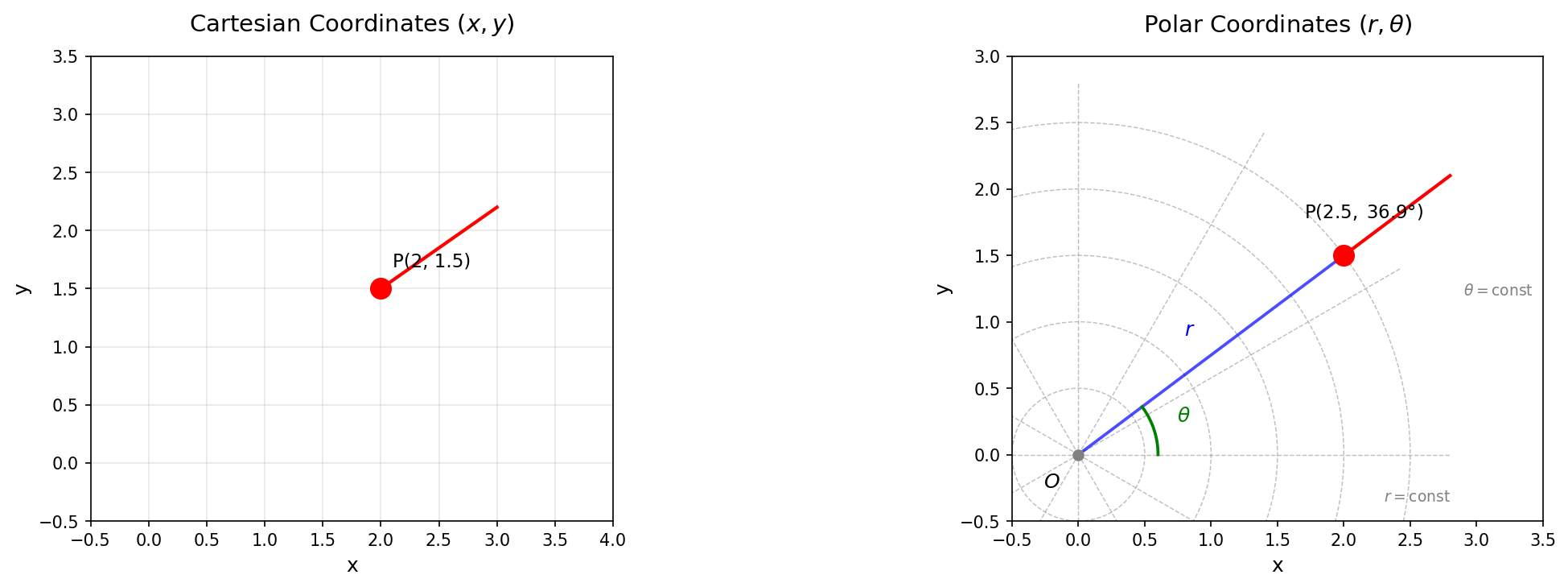
Fig. 6.1: Comparison of Cartesian and polar coordinates. The same point P is represented in Cartesian coordinates (left) and polar coordinates (right).
🔵 Kai: We covered this in high school.
🟡 Lina: Then let me ask you a question. What shapes do the coordinate lines of polar coordinates take—that is, the lines where "you fix \(r\) and vary only \(\theta\)" and the lines where "you fix \(\theta\) and vary only \(r\)"?
🔵 Kai: Lines of constant \(r\) are circles centered at the origin, and lines of constant \(\theta\) are straight lines extending from the origin.
🟡 Lina: Right. Because the coordinate lines aren't straight, we call them "curvilinear coordinates." But the important point is that just because the coordinate lines are curved doesn't mean the space itself is curved. Even if you draw polar coordinates on a sheet of paper, the paper remains flat, right?
⚪ Mei: That's the distinction between "curvature of coordinates" and "curvature of space" mentioned in §1. Polar coordinates are precisely a concrete example of that.
Spherical Coordinates (3 Dimensions)¶
🟡 Lina: Let's extend to 3 dimensions. Specifying a point \(P\) in space by its distance \(r\) from the origin, the angle \(\theta\) (theta, polar angle) from the \(z\)-axis, and the angle \(\varphi\) (phi, azimuthal angle) in the \(xy\)-plane gives us spherical coordinates. Take a look at Fig. 6.2 "Definition of spherical coordinates \((r, \theta, \varphi)\)".
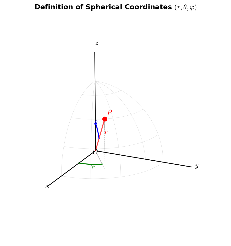
Fig. 6.2: Definition of spherical coordinates \((r, \theta, \varphi)\). The distance from origin O to point P is \(r\), the angle from the \(z\)-axis is the polar angle \(\theta\), and the angle between the projection onto the \(xy\)-plane and the \(x\)-axis is the azimuthal angle \(\varphi\).
The relationship with Cartesian coordinates is:
🔵 Kai: It's like latitude and longitude on Earth.
🟡 Lina: Yes. However, note that the polar angle \(\theta\) is measured from the North Pole, so it differs from geographic "latitude" by \(90°\).
6.3 Coordinate Transformations and the Jacobian Matrix¶
🟡 Lina: Now we get to the main topic. When you change coordinates, how does an "infinitesimal displacement" transform? The tool for handling this systematically is the Jacobian matrix.
Transformation of Infinitesimal Displacements¶
🟡 Lina: Let's find the relationship between the infinitesimal displacements \((dx, dy)\) in Cartesian coordinates \((x, y)\) and \((dr, d\theta)\) in polar coordinates \((r, \theta)\). Since \(x = r\cos\theta\) is a function of two variables \(r\) and \(\theta\), when \(r\) and \(\theta\) both change by small amounts simultaneously, how much does \(x\) change? For a single-variable function \(f(x)\), we could write \(df = f'(x)\,dx\). The same idea works for two variables—if the changes are sufficiently small, we can independently calculate the change from varying \(r\) alone and the change from varying \(\theta\) alone, then add them together. This operation of "adding the contributions from each variable to express the total change" is called the total differential:
Here \(\dfrac{\partial x}{\partial r}\) is "the rate of change of \(x\) when only \(r\) changes while \(\theta\) is held fixed" (partial derivative), and \(\dfrac{\partial x}{\partial \theta}\) is "the rate of change of \(x\) when only \(\theta\) changes while \(r\) is held fixed." It's a natural extension of the single-variable differential \(df = f'(x)\,dx\).
🔵 Kai: Ah, "adding the contributions from each direction" works because the changes are small enough for superposition to hold.
🟡 Lina: Exactly. Computing explicitly:
Similarly, from \(y = r\sin\theta\):
In matrix form:
⚪ Mei: So this single matrix encodes the entire "transformation from infinitesimal displacements in polar coordinates to infinitesimal displacements in Cartesian coordinates."
🟡 Lina: This \(2 \times 2\) matrix on the right-hand side is called the Jacobian matrix. In general, we sometimes label coordinates with numbers like \((x^1, x^2)\), \((u^1, u^2)\). In this example, \((x^1, x^2) = (x, y)\) corresponds to Cartesian coordinates and \((u^1, u^2) = (r, \theta)\) to polar coordinates. Note that the superscript numbers are not exponents but coordinate labels (indices). \(x^2\) does not mean "\(x\) squared" but "the 2nd coordinate" (i.e., \(y\)). It's confusing, but this notation is standard in tensor calculus.
Using this notation, when coordinates \((x^1, x^2)\) are written as functions of coordinates \((u^1, u^2)\)—meaning "given \(u\) coordinates, the \(x\) coordinates are determined"—
gives the components of the Jacobian matrix.
🔵 Kai: \(x^2\) being "the 2nd coordinate" rather than "\(x\) squared"... that's going to be confusing at first. Won't it get mixed up with exponentiation?
🟡 Lina: You have to judge from context. But in practice, when labeling coordinates, the index is always written as a superscript, so for polar coordinates you'd write \(u^1 = r\), \(u^2 = \theta\). When you see "\(u^2 = \theta\)," you wouldn't think "\(u\) squared equals theta," right? When exponentiation is needed, we use parentheses like \((u^1)^2\).
⚪ Mei: So each component represents "how much the old coordinate moves when you slightly move the new coordinate."
🔵 Kai: The key point is that the components of this matrix are not constants. They depend on \(r\) and \(\theta\).
🟡 Lina: Good observation. The Lorentz transformation matrix had constant entries, but for general coordinate transformations the transformation matrix varies from place to place. This is the essentially new feature of curvilinear coordinates. Looking at Fig. 6.3 "The same 2-dimensional plane covered by two coordinate systems", you can see that while the Cartesian mesh is evenly spaced, the polar coordinate mesh changes spacing depending on location.
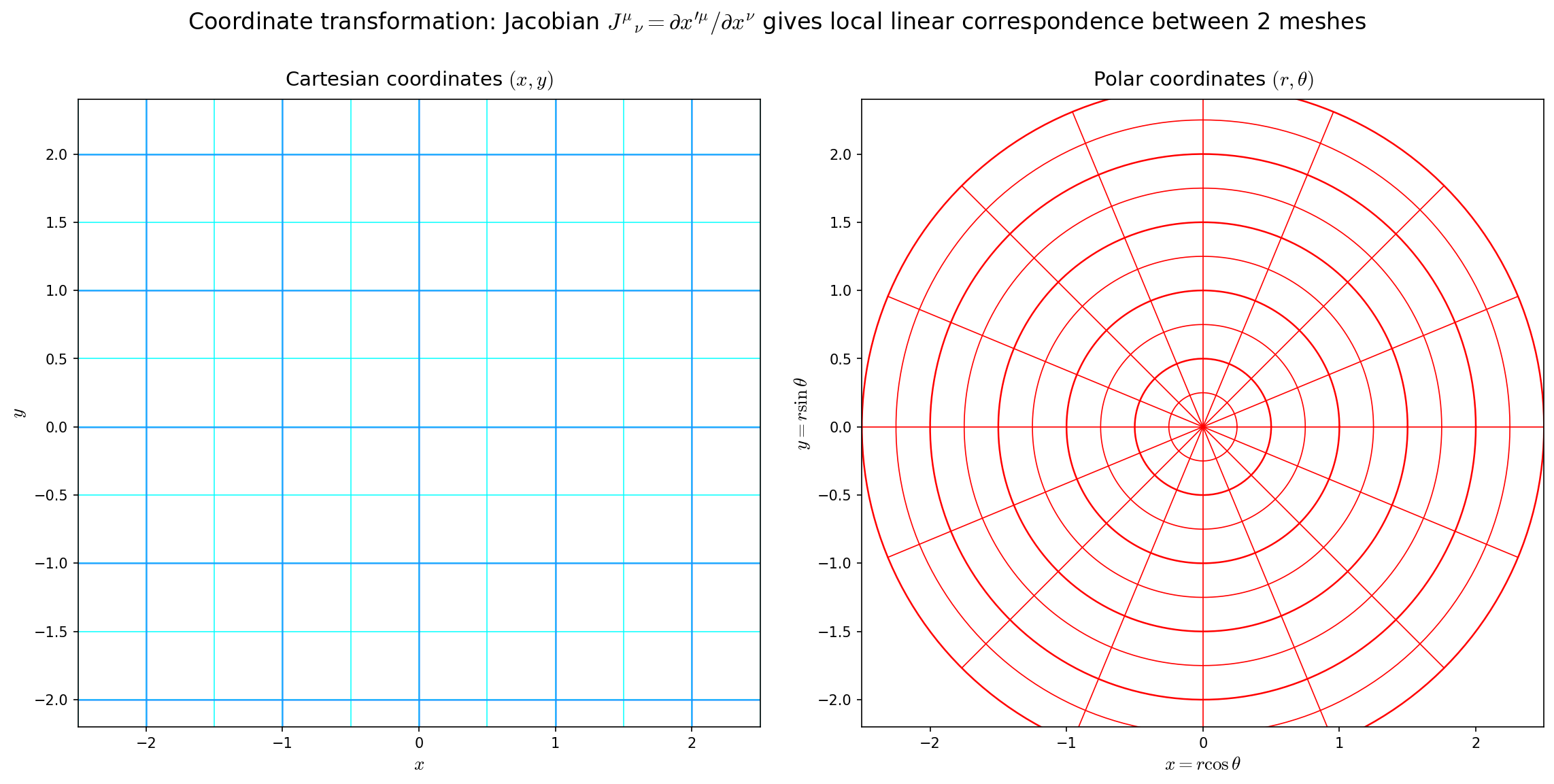
Fig. 6.3: The same 2-dimensional plane covered by two coordinate systems. The Cartesian mesh (left) is evenly spaced, parallel, and orthogonal; the polar mesh (right) is arranged radially around the origin. The linear transformation connecting the same infinitesimal displacement measured as (a) \((dx, dy)\) or (b) \((dr, d\theta)\) is the Jacobian matrix \(J^i{}_j = \partial x^i/\partial u^j\). The fact that this matrix varies from place to place is the essential characteristic of curvilinear coordinates.
✅ Comprehension Check: What is the crucial difference between the transformation matrix of a Lorentz transformation and the Jacobian matrix of a general curvilinear coordinate transformation?
Answer
The Lorentz transformation matrix is constant (independent of position), but the Jacobian matrix of a general curvilinear coordinate transformation depends on the coordinate values (position). This is the essentially new feature of curvilinear coordinates.
Inverse Transformation and the Inverse of the Jacobian Matrix¶
🟡 Lina: Let's also consider the transformation in the reverse direction. Differentiating \(r = \sqrt{x^2 + y^2}\) and \(\theta = \arctan(y/x)\):
(Hint: Since \(r = \sqrt{x^2 + y^2} = (x^2 + y^2)^{1/2}\), by the chain rule \(\partial r/\partial x = \frac{1}{2}(x^2+y^2)^{-1/2}\cdot 2x = x/\sqrt{x^2+y^2}\). Similarly \(\partial r/\partial y = y/\sqrt{x^2+y^2}\). For \(\theta\), in the region \(x > 0\) we set \(\theta = \arctan(y/x)\) and apply the derivative formula for inverse trigonometric functions \((\arctan u)' = 1/(1 + u^2)\) (see the collapsible supplement just below for the derivation) along with the chain rule. For \(\partial\theta/\partial x\): setting \(u = y/x\) gives \(\partial u/\partial x = -y/x^2\), so \(\partial\theta/\partial x = \frac{1}{1+(y/x)^2}\cdot(-y/x^2) = -y/(x^2+y^2)\). For \(\partial\theta/\partial y\): similarly \(u = y/x\) with \(\partial u/\partial y = 1/x\), so \(\partial\theta/\partial y = \frac{1}{1+(y/x)^2}\cdot(1/x) = x/(x^2+y^2)\).)
::: {.callout-note collapse="true" title="Supplement: Derivation of \((\arctan u)' = 1/(1+u^2)\)"} Let \(\theta = \arctan u\), so \(\tan\theta = u\). Differentiating both sides with respect to \(u\): the left side gives \(\frac{1}{\cos^2\theta}\cdot\frac{d\theta}{du}\) by the chain rule, and the right side is 1. Therefore \(\frac{d\theta}{du} = \cos^2\theta\). Since \(1 + \tan^2\theta = 1/\cos^2\theta\) (obtained by dividing \(\sin^2\theta + \cos^2\theta = 1\) by \(\cos^2\theta\)), we have \(\cos^2\theta = 1/(1 + u^2)\). Thus \((\arctan u)' = 1/(1 + u^2)\). :::
In matrix form:
🟡 Lina: Let's multiply these two Jacobian matrices together. They should be inverses of each other. Mei, could you compute it?
⚪ Mei: Let me try.
\((1,1)\) entry: \(\cos\theta \cdot \cos\theta + (-r\sin\theta) \cdot \left(-\dfrac{\sin\theta}{r}\right) = \cos^2\theta + \sin^2\theta = 1\)
\((1,2)\) entry: \(\cos\theta\sin\theta - r\sin\theta \cdot \dfrac{\cos\theta}{r} = 0\)
\((2,1)\) entry: \(\sin\theta \cdot \cos\theta + r\cos\theta \cdot \left(-\dfrac{\sin\theta}{r}\right) = \sin\theta\cos\theta - \sin\theta\cos\theta = 0\)
\((2,2)\) entry: \(\sin^2\theta + r\cos\theta \cdot \dfrac{\cos\theta}{r} = 1\)
The result is the identity matrix. So the two Jacobian matrices are inverses of each other.
🟡 Lina: Exactly. This is a theorem that holds in general. It can be proven in one line using the chain rule. Let me take this opportunity to review the Einstein summation convention—the rule introduced in Ch. 2 that "when the same index appears both upstairs and downstairs in the same expression, sum over that index." For example, \(A^j B_j\) means \(\sum_j A^j B_j = A^1 B_1 + A^2 B_2 + \cdots\). In 2 dimensions, \(A^j B_j = A^1 B_1 + A^2 B_2\). Since you don't have to write \(\sum\) every time, this is used as standard practice in tensor calculations. In this chapter we'll also apply it to indices on partial derivatives, so make sure you remember the rule.
🔵 Kai: "The same index upstairs and downstairs"—how do you determine which is up and which is down? It's clear when they're explicitly written up and down like in the Jacobian matrix \(J^i{}_j\), but what about with partial derivatives?
🟡 Lina: Good question. For partial derivatives, the rule is: an index in the numerator counts as "up," and an index in the denominator counts as "down." For example, in \(\dfrac{\partial x^i}{\partial u^j}\), \(i\) is in the numerator so it's "up," and \(j\) is in the denominator so it's "down." Intuitively, \(dx^i\) is a coordinate displacement carrying an upper index, while \(\partial u^j\) is in the denominator so it becomes lower. Why this distinction is fundamental will become clear in the next chapter when we systematically study "contravariant and covariant," but for now just remember "numerator is up, denominator is down."
🔵 Kai: I see, so in \(\dfrac{\partial x^i}{\partial u^j}\), \(i\) is up and \(j\) is down... and in \(\dfrac{\partial u^j}{\partial x^k}\), \(j\) is in the numerator so it's up. That means \(j\) appears both down and up, so we sum over \(j\)—right?
🟡 Lina: Exactly. Using this convention, the chain rule can be written as:
Look at the left side. In the first factor \(\dfrac{\partial x^i}{\partial u^j}\), \(j\) is down (denominator); in the second factor \(\dfrac{\partial u^j}{\partial x^k}\), \(j\) is up (numerator)—so \(j\) appears both up and down, meaning we sum over \(j\). Expanded, it means \(\sum_{j} \dfrac{\partial x^i}{\partial u^j}\dfrac{\partial u^j}{\partial x^k}\).
⚪ Mei: Just by tracking which indices are up and down, "where the sum goes" is determined automatically. Once you get used to it, it seems easier than writing \(\sum\).
🟡 Lina: Writing it out explicitly in 2 dimensions, for example with \(i = 1\), \(k = 1\):
This says that the operation of "going from \(x\) through \((r, \theta)\) back to \(x\) itself" is the identity transformation. The symbol \(\delta^i_k\) appearing on the right is called the Kronecker delta, defined as 1 if \(i = k\) and 0 if \(i \neq k\). In other words, "if you differentiate \(x^i\) with respect to \(x^k\), you get 1 for the same coordinate (\(i = k\)) and 0 for different coordinates (\(i \neq k\))"—a completely obvious statement written in symbolic form. Concretely, with \(x^1 = x\), \(x^2 = y\): \(\partial x / \partial x = 1\), \(\partial x / \partial y = 0\)—since \(x\) and \(y\) are independent coordinates, changing one doesn't affect the other. In 2 dimensions, \(\delta^1_1 = 1\), \(\delta^1_2 = 0\), \(\delta^2_1 = 0\), \(\delta^2_2 = 1\), so written as a matrix it's just the identity matrix \(\begin{pmatrix}1 & 0\\0 & 1\end{pmatrix}\). The indices being split between upper and lower positions simply matches the index positions on the left side.
🔵 Kai: So the "forward transformation matrix" and the "backward transformation matrix" are always inverses of each other.
✅ Comprehension Check: What is the relationship between the Jacobian matrix of a coordinate transformation \(x^i(u^j)\) and the Jacobian matrix of the inverse transformation \(u^j(x^i)\)?
Answer
They are inverses of each other. This follows from the chain rule: \(\frac{\partial x^i}{\partial u^j}\frac{\partial u^j}{\partial x^k} = \delta^i_k\).
✅ Comprehension Check: What is a Jacobian matrix?
Answer
A matrix whose components are the partial derivatives \(J^i{}_j = \partial x^i / \partial u^j\) of the coordinate transformation \(x^i = x^i(u^1, u^2, \ldots)\). It describes how infinitesimal displacements transform. Unlike the Lorentz transformation, for general coordinate transformations the components vary from place to place.
📝 Exercises:
6.4 Expressing "Distance" in Coordinates—Introducing the Metric Tensor¶
Motivation: Distance Doesn't Change When Coordinates Change¶
🟡 Lina: Now we come to the heart of this chapter. One of the most fundamental quantities in physics is "the distance between two points." Distance is independent of the choice of coordinates—the distance from Tokyo to New York doesn't change no matter how you draw the map, right?
🔵 Kai: Yes, obviously.
🟡 Lina: But the formula for computing the distance does change with the coordinates. In Cartesian coordinates, it's simply the Pythagorean theorem:
So what about in polar coordinates? Substitute \(dx = \cos\theta\,dr - r\sin\theta\,d\theta\) and \(dy = \sin\theta\,dr + r\cos\theta\,d\theta\).
⚪ Mei: Let me compute this.
Expanding the first term:
Expanding the second term:
🔵 Kai: Ah, the \(dr\,d\theta\) terms have opposite signs so they should cancel!
⚪ Mei: Exactly. Adding them together, the cross terms cancel:
🔵 Kai: Oh, that came out nice and clean! But... there's an \(r^2\) in front of \(d\theta^2\). In Cartesian coordinates it was \(dx^2 + dy^2\) with all coefficients equal to 1.
🟡 Lina: Right. This is the crucial point. In polar coordinates, the actual distance traveled when you change \(\theta\) by 1 radian depends on the distance \(r\) from the origin. At \(r = 1\), one radian gives a distance of 1, but at \(r = 10\), one radian gives a distance of 10. That's why \(d\theta^2\) gets a "weight" of \(r^2\) in front of it.
🔵 Kai: So you're saying that the same \(d\theta\) corresponds to different "actual distances" depending on where you are?
🟡 Lina: Exactly. This is the true nature of what "the ruler changes from place to place" means. Looking at Fig. 6.4 "Meaning of the metric in polar coordinates", you can clearly see that the same \(d\theta\) produces a longer arc length when \(r\) is larger.
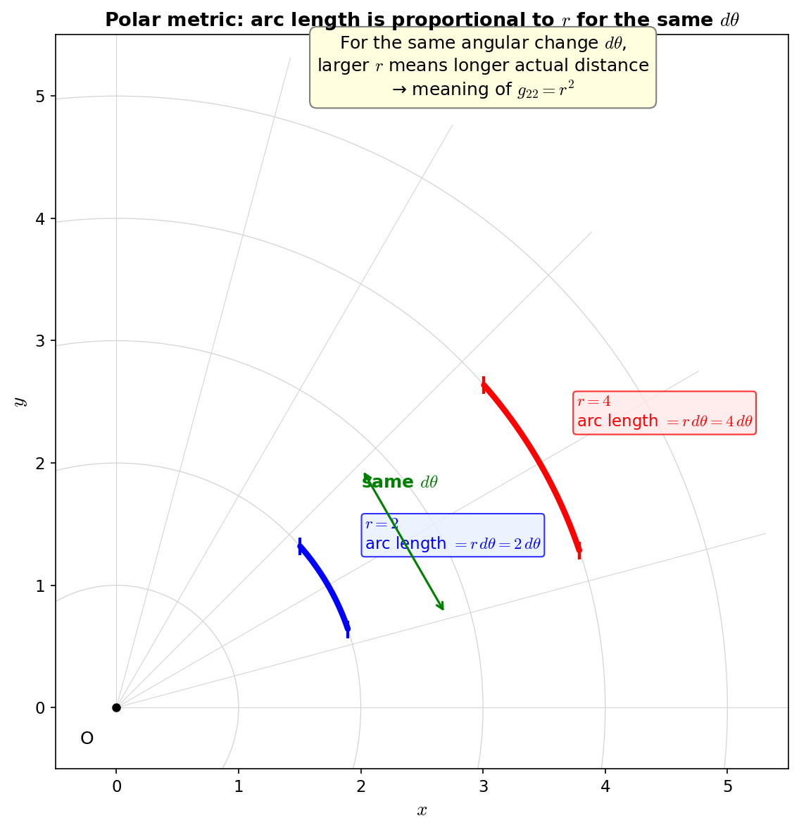
Fig. 6.4: Meaning of the metric in polar coordinates. Even for the same angular change \(d\theta\), the actual arc length \(r\,d\theta\) increases with the distance \(r\) from the origin. This is the geometric meaning of \(g_{22} = r^2\).
✅ Comprehension Check: In the polar coordinate line element \(ds^2 = dr^2 + r^2\,d\theta^2\), what is the physical meaning of the \(r^2\) in front of \(d\theta^2\)?
Answer
It means that even if you change the angle \(\theta\) by the same amount, the actual distance traveled is larger when the distance \(r\) from the origin is larger. In other words, the tick spacing of the "ruler" in the \(\theta\) direction changes in proportion to \(r\).
Definition of the Metric Tensor \(g_{ij}\)¶
🟡 Lina: The tool for writing this "distance formula" in general form is the metric tensor \(g_{ij}\).
Using coordinates \((u^1, u^2)\)—for polar coordinates, \((u^1, u^2) = (r, \theta)\)—the square of the infinitesimal distance is written as
Here we're using the Einstein summation convention introduced in §3—look at \(g_{ij}\,du^i\,du^j\). The index \(i\) appears as a lower index in \(g_{ij}\) and as an upper index in \(du^i\)—that is, the same index \(i\) appears both up and down, so we sum over \(i\). Similarly, \(j\) appears down in \(g_{ij}\) and up in \(du^j\), so we sum over \(j\) as well. This means \(g_{ij}\,du^i\,du^j = \sum_{i=1}^{2}\sum_{j=1}^{2} g_{ij}\,du^i\,du^j\) in shorthand. In 2 dimensions (where \(i, j\) each run from 1 to 2), writing out all four terms:
🔵 Kai: Are \(g_{12}\) and \(g_{21}\) separate components?
🟡 Lina: Good question. Actually, since \(du^1\,du^2 = du^2\,du^1\) (just multiplication of numbers), we can write \(g_{12}\,du^1\,du^2 + g_{21}\,du^2\,du^1 = (g_{12} + g_{21})\,du^1\,du^2\). Only "the sum of \(g_{12}\) and \(g_{21}\)" has physical meaning. So we adopt the convention that \(g_{12} = g_{21}\) is always symmetric. In general, in \(n\) dimensions, the metric tensor satisfies the symmetry condition \(g_{ij} = g_{ji}\). Since it's a symmetric matrix, an \(n \times n\) metric has \(n(n+1)/2\) independent components—\(n\) diagonal entries and \(n(n-1)/2\) upper-triangular entries. In 2 dimensions that's \(g_{11}, g_{12} = g_{21}, g_{22}\)—3 components. In 4-dimensional spacetime, \(n = 4\) gives \(4 \times 5 / 2 = 10\) components. In the previous chapter we learned that "gravity is the curvature of spacetime." What describes how spacetime curves—that is, "how the ruler changes from place to place"—is precisely this metric tensor \(g_{\mu\nu}\).
🔵 Kai: 3 in 2 dimensions, 10 in 4 dimensions... that increases quickly. In Newtonian gravity, the potential \(\Phi\) was just a single function. Why does it go from 1 to 10—what becomes so much more complicated?
🟡 Lina: Newtonian gravity only described "the strength of the attractive force between masses," but general relativity describes the geometry of the entire spacetime including time dilation and spatial distortion. So one function isn't enough and we need 10—it means the description of gravity becomes that much richer.
⚪ Mei: I see, because we're describing distortions of both time and space, many components are needed.
🟡 Lina: Now, let's get back on track. Try reading off the specific components of the metric tensor for polar coordinates.
⚪ Mei: For polar coordinates, \(ds^2 = dr^2 + r^2\,d\theta^2\), so by comparison:
Written as a matrix:
🔵 Kai: What does \(g_{ij}\) look like in Cartesian coordinates?
🟡 Lina: Since \(ds^2 = dx^2 + dy^2\):
The identity matrix—that is, the Kronecker delta. A coordinate system in which the metric tensor is the identity matrix is a Cartesian coordinate system.
🔵 Kai: I see. Cartesian coordinates are "specially simple" because the metric tensor is a constant identity matrix. So conversely, in a coordinate system where the metric tensor isn't the identity matrix, the distance calculation just becomes more tedious, but the physical content doesn't change at all?
🟡 Lina: If you're just changing coordinates within flat space, that's correct—only the appearance of the calculation changes, not the physics. But in genuinely curved space, things are different. Let's see that next.
🔵 Kai: What changes in "genuinely curved space"... I'm curious.
✅ Comprehension Check: Why is the metric tensor \(g_{ij}\) symmetric (\(g_{ij} = g_{ji}\))?
Answer
In \(ds^2 = g_{ij}\,du^i\,du^j\), since \(du^i\,du^j = du^j\,du^i\) (just a product of numbers), only the sum of \(g_{ij}\) and \(g_{ji}\) has physical meaning. Therefore we adopt the convention that it is always symmetric.
✅ Comprehension Check: Write the metric tensor \(g_{ij}\) for polar coordinates as a matrix.
Answer
\(g_{ij} = \begin{pmatrix} 1 & 0 \\ 0 & r^2 \end{pmatrix}\). The component \(g_{22} = r^2\) indicates that "the actual distance per unit coordinate change in the \(\theta\) direction is proportional to \(r\)."
Metric Tensor in Spherical Coordinates¶
🟡 Lina: Let's do the same thing for 3-dimensional spherical coordinates \((r, \theta, \varphi)\). We rewrite \(dx^2 + dy^2 + dz^2\) in spherical coordinates. The approach is the same as in 2 dimensions—find the total differential of each of \(x, y, z\), square them, and add them up. Since \(dx = \sin\theta\cos\varphi\,dr + r\cos\theta\cos\varphi\,d\theta - r\sin\theta\sin\varphi\,d\varphi\) involves 3 variables, there are more terms, but the mechanism is exactly the same as in 2 dimensions. When you expand \(dx^2 + dy^2 + dz^2\), cross terms (\(dr\,d\theta\), \(dr\,d\varphi\), \(d\theta\,d\varphi\) terms) appear, but when you add the contributions from all three of \(x, y, z\), they all cancel thanks to \(\sin^2\alpha + \cos^2\alpha = 1\).
🔵 Kai: The cross terms canceled cleanly in 2 dimensions too, and the same thing happens in 3 dimensions.
🟡 Lina: Hint: for example, looking at the coefficient of \(dr\,d\theta\), from \(dx^2\) we get \(2r\sin\theta\cos\theta\cos^2\varphi\), from \(dy^2\) we get \(2r\sin\theta\cos\theta\sin^2\varphi\), and from \(dz^2\) we get \(-2r\sin\theta\cos\theta\). Adding these gives \(2r\sin\theta\cos\theta(\cos^2\varphi + \sin^2\varphi - 1) = 0\), so it vanishes. The \(dr\,d\varphi\) cross term similarly vanishes by the same \(\cos^2\varphi + \sin^2\varphi - 1 = 0\) type cancellation, and for \(d\theta\,d\varphi\), the contribution from \(dx^2\) is \(-2r^2\sin\theta\cos\theta\sin\varphi\cos\varphi\) and from \(dy^2\) is \(+2r^2\sin\theta\cos\theta\sin\varphi\cos\varphi\), which cancel each other (from \(dz^2\) there's no contribution containing \(d\varphi\), so it's zero). You can verify all the calculations in exercise Problem M-2. Derivation of the Line Element in Spherical Coordinates. The result is:
⚪ Mei: Therefore the metric tensor is:
🔵 Kai: The \(r^2\sin^2\theta\) in front of \(d\varphi^2\) is because... ah, near the equator (\(\theta = \pi/2\)) changing longitude by 1 radian moves you by \(r\), but near the North Pole (\(\theta \approx 0\)) you barely move at all! But at \(\theta = 0\) (the North Pole), \(g_{33} = 0\). Doesn't having a zero component of the metric tensor cause problems?
🟡 Lina: Good question. \(g_{33} = 0\) means "changing \(\varphi\) gives zero displacement"—in other words, at the North Pole all meridians converge to a single point, so differences in longitude have no physical meaning. The coordinate \(\varphi\) is defined there, but the tick spacing of the "ruler" in the \(\varphi\) direction becomes zero at that point. This is called a coordinate singularity—the space itself isn't broken; using different coordinates describes it without problems. It's easy to understand thinking about Earth. On the equator, 1° of longitude corresponds to about 111 km, but at latitude 60° N it's only about 56 km. The \(\sin^2\theta\) expresses this "position-dependent difference in distances."
✅ Comprehension Check: What is the geometric reason that the 3D spherical coordinate metric tensor component \(g_{33} = r^2\sin^2\theta\) depends on \(\theta\)?
Answer
The radius of the circle in the \(\varphi\) direction is \(r\sin\theta\), which varies with the polar angle \(\theta\). It is maximum at the equator (\(\theta = \pi/2\)) and zero at the poles (\(\theta = 0\) or \(\pi\)).
🟡 Lina: We've now found the metric tensor in three coordinate systems. Mei, could you summarize them?
⚪ Mei: Let me try. The form varies quite a lot depending on the coordinate system.
Table 6.1: Comparison of metric tensors in different coordinate systems
| Coordinate system | Line element \(ds^2\) | \(g_{ij}\) (matrix form) | Curvature of space |
|---|---|---|---|
| 2D Cartesian \((x, y)\) | \(dx^2 + dy^2\) | \(\mathrm{diag}(1, 1)\) | Flat |
| 2D polar \((r, \theta)\) | \(dr^2 + r^2\,d\theta^2\) | \(\mathrm{diag}(1, r^2)\) | Flat |
| 3D spherical \((r, \theta, \varphi)\) | \(dr^2 + r^2\,d\theta^2 + r^2\sin^2\theta\,d\varphi^2\) | \(\mathrm{diag}(1, r^2, r^2\sin^2\theta)\) | Flat |
📝 Exercises:
- Reading metric tensors and inverse metrics → Problem B-2. Inverse Metric in 3D Spherical Coordinates, Problem B-3. Matrix Representation of a General 2-Dimensional Metric, Problem B-4. Metric Tensor on a Sphere at a Specific Point
The Metric on a Sphere—An Example of Curved Space¶
🟡 Lina: Everything up to now has just been flat space written in curvilinear coordinates. Next, let's look at an example of genuinely curved space. Describing a sphere of radius \(a\) (a 2-dimensional curved space) using coordinates \((u^1, u^2) = (\theta, \varphi)\):
The metric tensor is—since it's 2-dimensional, a \(2 \times 2\) matrix, with \((u^1, u^2) = (\theta, \varphi)\) in order:
🔵 Kai: Wait, isn't this just taking the \(g_{22}\) and \(g_{33}\) parts of the 3D spherical coordinates and setting \(r = a\) (constant)?
🟡 Lina: Good observation. A sphere is a 2-dimensional surface embedded in 3-dimensional space, so the metric of the "cross-section" obtained by fixing \(r\) in the 3D metric becomes the metric of the sphere.
🔵 Kai: But even for polar coordinates in flat space, the metric tensor depended on position (\(g_{22} = r^2\)). It also depends on position for the sphere. Can you really say space is "curved" just because the metric tensor depends on position?
🟡 Lina: Good question. Actually, just because the metric tensor depends on position doesn't mean you can determine whether the space is curved. Even in flat space, using curvilinear coordinates makes \(g_{ij}\) position-dependent. In genuinely curved space, no matter what coordinates you use, you cannot make \(g_{ij}\) constant (globally). Determining this requires the Riemann curvature tensor, which we'll learn in a later chapter. For now, just remember that "metric tensor depends on position ≠ space is curved."
⚪ Mei: So "curvature of coordinates" and "curvature of space" are separate concepts, and we still need a tool to distinguish them.
✅ Comprehension Check: When the metric tensor components depend on position, what is needed to determine whether the space is truly curved?
Answer
The Riemann curvature tensor is needed. The metric tensor depending on position alone cannot determine whether space is curved (even in flat space, using curvilinear coordinates makes the metric position-dependent).
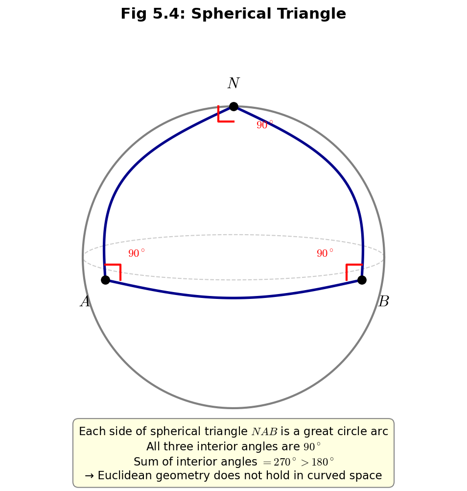 Fig. 6.5: Spherical triangle NAB. All three interior angles are 90°, so the sum is 270° > 180°. An intuitive example showing that Euclidean geometry fails in curved space.
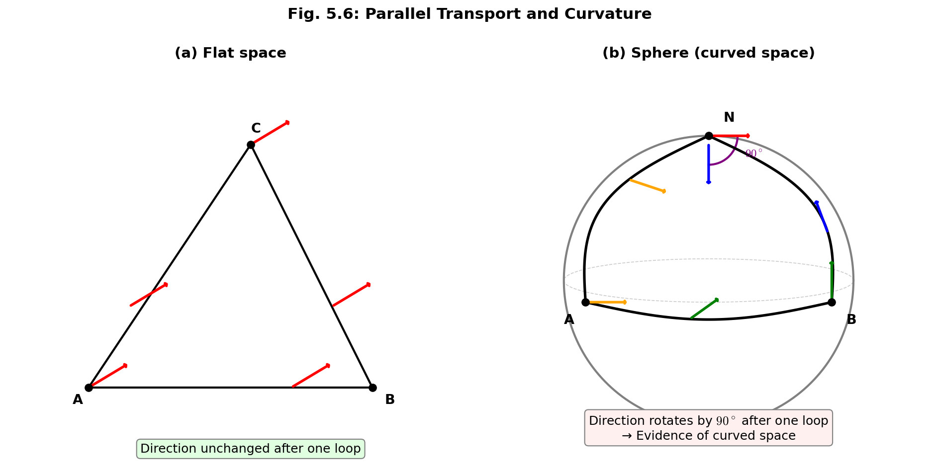 Fig. 6.6: In flat space, a vector returns to its original direction after being transported around a loop. On a sphere, it rotates by 90°. This is the essential method for detecting "curvature of space" and gives the intuitive meaning of the Riemann curvature tensor.
6.5 Transformation Law for the Metric Tensor¶
Deriving the Transformation Law from Invariance of Distance¶
🟡 Lina: The most important property of the metric tensor is that when you change coordinates, the components transform in such a way that the distance \(ds^2\) remains unchanged. Let's derive this in equations.
Let the metric in one coordinate system \((x^1, x^2)\) be \(g_{ij}\), and the metric in another coordinate system \((u^1, u^2)\) be \(g'_{ij}\). Here \((x^1, x^2)\) is not necessarily Cartesian—any coordinate system can serve as the starting point. Since distance doesn't depend on the choice of coordinates:
Now substitute \(dx^i = \dfrac{\partial x^i}{\partial u^k}\,du^k\) into the left side. Similarly write \(dx^j = \dfrac{\partial x^j}{\partial u^l}\,du^l\). We use a different letter \(l\) here rather than \(k\) because \(k\) is already being used as a dummy index (summation index) in the expansion of \(dx^i\)—if we also used \(k\) for the expansion of \(dx^j\), the index \(k\) would appear more than twice in a single expression, making "how many times to sum over \(k\)" ambiguous. Using a different letter \(l\) makes it clear that \(k\) and \(l\) each independently run from 1 to 2 as a double sum (\(\sum_k \sum_l\)). Then:
On the other hand, the right side was \(ds^2 = g'_{kl}\,du^k\,du^l\). So:
🔵 Kai: Both sides have the same \(du^k\,du^l\) multiplied, so the coefficients inside should be equal... right?
🟡 Lina: Intuitively, that's correct. However, since \(du^k\,du^l\) is just a product of numbers (scalars), we need to carefully show this by using the fact that "it holds for any direction." This equation must hold for any choice of infinitesimal displacement \((du^1, du^2)\). From this we'll show that "the coefficients are equal." Let's first build intuition with a single-variable analogy. If \(ax^2 + bx + c = a'x^2 + b'x + c'\) holds for all \(x\), then substituting \(x = 0\) gives \(c = c'\), substituting \(x = 1\) gives \(a + b = a' + b'\), and substituting \(x = -1\) gives \(a - b = a' - b'\)—just trying 3 values is enough to determine \(a = a'\), \(b = b'\), \(c = c'\). The point is "if you can create as many independent conditions as unknowns, everything is determined." The same idea works in two variables. As we saw in §4, \(g'_{kl}\) is symmetric (\(g'_{12} = g'_{21}\)), so the independent components to determine are only \(g'_{11}\), \(g'_{12}\), \(g'_{22}\)—3 unknowns. To determine 3 unknowns, trying 3 directions suffices—the same as solving a system of equations. Let's do it concretely:
- Direction 1: Set \(du^2 = 0\) and vary only \(du^1\). Then both sides become \(g'_{11}(du^1)^2 = \bigl(g_{ij}\frac{\partial x^i}{\partial u^1}\frac{\partial x^j}{\partial u^1}\bigr)(du^1)^2\). Since \((du^1)^2 \neq 0\), we can divide by it to determine \(g'_{11}\)
- Direction 2: Setting \(du^1 = 0\) similarly determines \(g'_{22}\)
- Direction 3: To determine \(g'_{12}\), we need a direction where both \(du^1\) and \(du^2\) are nonzero. The simplest choice is \(du^1 = du^2 = \epsilon\) (the same small quantity). Then the left side is \((g'_{11} + 2g'_{12} + g'_{22})\epsilon^2\), and the right side is
Dividing by \(\epsilon^2 \neq 0\) and subtracting the terms corresponding to \(g'_{11}\) and \(g'_{22}\) determined in Directions 1 and 2, we're left with \(2g'_{12} = 2g_{ij}\frac{\partial x^i}{\partial u^1}\frac{\partial x^j}{\partial u^2}\), so \(g'_{12}\) is also uniquely determined.
⚪ Mei: Just trying 3 directions determines all the independent components—it really is the same idea as comparing polynomial coefficients.
🔵 Kai: Wait a moment. We determine \(g'_{11}\) and \(g'_{22}\) from Directions 1 and 2, then \(g'_{12}\) from Direction 3—so choosing 3 directions determines all 3 unknowns. But the choice \(du^1 = du^2 = \epsilon\) in Direction 3 was just for convenience—would a different combination give the same \(g'_{12}\)?
🟡 Lina: That's right. With 3 independent components \(g'_{11}\), \(g'_{12}\), \(g'_{22}\) all uniquely determined, and since a symmetric matrix only has 3 independent components, determining those 3 determines the entire matrix.
::: {.callout-note collapse="true" title="Supplement: Why 3 directions suffice"} Let's verify—if we substituted a different direction, say \(du^1 = 1\), \(du^2 = 3\), the left side would be \(g'_{11} + 6g'_{12} + 9g'_{22}\), and the right side would give the same value. This is because the 3 components are already determined by Directions 1–3, and the value of any quadratic form in any direction is determined by just these 3 components. In other words, if two quadratic forms agree for 3 independent directions, they agree for all directions—exactly the same logic as two quadratic functions being identical if they agree at 3 points. :::
To summarize:
🔵 Kai: I see, in 2 dimensions the independent components are 3 (because of symmetry), and choosing 3 directions determines them all... so in \(n\) dimensions you'd just choose enough directions for the number of independent components? But choosing a "diagonal direction" like \(du^1 = du^2 = \epsilon\) feels a bit tricky. Would other directions work too?
🟡 Lina: Good question. Other directions—for example \(du^1 = \epsilon\), \(du^2 = 2\epsilon\)—would work just as well. The point is that after determining \(g'_{11}\) and \(g'_{22}\) first, you just need to choose any one direction where both \(du^1\) and \(du^2\) are nonzero to determine \(g'_{12}\). No matter which direction you choose, you'll get the same \(g'_{12}\)—that's a consequence of "it holds for any direction." In \(n\) dimensions, choosing \(n(n+1)/2\) directions determines all components.
🔵 Kai: So because the number of equations (directions you can choose) is at least as large as the number of unknowns (independent components), everything is determined. Same idea as solving a system of equations.
🟡 Lina: Exactly. Intuitively, "the distance agrees no matter what direction you take the infinitesimal displacement" requires all coefficients in the distance formula to agree—just like if two polynomials are equal for all \(x\), the coefficients at each degree must be equal. This is the transformation law for the metric tensor. Two factors of the Jacobian matrix component \(\dfrac{\partial x^i}{\partial u^k}\) appear. In tensor language, this shows that the metric tensor is a rank-2 covariant tensor—a tensor with two lower indices. Recall from Ch. 2 that "the rank of a tensor is the number of indices." \(g_{kl}\) has two lower indices so it's "rank 2," and having two Jacobian matrices in the transformation law is the manifestation of this.
🔵 Kai: What does "covariant" mean?
🟡 Lina: Good question. There are two types of tensors distinguished by their transformation laws. A tensor whose transformation law uses \(\dfrac{\partial x^i}{\partial u^k}\)—that is, "the old coordinates differentiated with respect to the new coordinates"—is called a covariant tensor, and its indices are written downstairs. For example, the metric tensor's transformation law \(g'_{kl} = \dfrac{\partial x^i}{\partial u^k}\dfrac{\partial x^j}{\partial u^l}\,g_{ij}\) is exactly this form. Conversely, one that uses \(\dfrac{\partial u^k}{\partial x^i}\) (the inverse matrix components) is called a contravariant tensor, and its indices are written upstairs—for example, the infinitesimal displacement \(du^k = \dfrac{\partial u^k}{\partial x^i}\,dx^i\) transforms contravariantly.
🔵 Kai: Why is it necessary to distinguish between two types?
🟡 Lina: Because different physical quantities "transform differently when you change coordinates." Let's think about the most intuitive example. Suppose you change length units from meters to centimeters—this is the simplest coordinate transformation of "making the coordinate scale uniformly 100 times finer." The same displacement gets a numerical value 100 times larger (\(du^k\) becomes larger)—when the coordinate scale becomes finer, a larger number is needed to represent the same distance. For example, a displacement of 3 m becomes 300 cm—the number increases. This is a contravariant transformation.
🔵 Kai: Is there something that gets smaller in the opposite way?
🟡 Lina: Yes. Think about "temperature change per meter." If temperature increases by 2°C for every 1 m, then per 1 cm it increases by only 0.02°C—the numerical value becomes 1/100 (the gradient \(\partial f/\partial u^k\) gets smaller). When the scale becomes finer, the change per tick mark becomes smaller. This is a covariant transformation. So for the same coordinate transformation, some quantities get numerically larger (contravariant, upper index) and some get smaller (covariant, lower index)—the "direction" of transformation is opposite.
⚪ Mei: Displacement gets numerically larger when the scale becomes finer, while gradient gets smaller—because the direction of transformation is opposite, they're called "contravariant" and "covariant."
🟡 Lina: Right. The unit change just discussed is the simplest example where the scale changes uniformly, but the same thing happens when the scale varies from place to place, as in polar coordinates. For example, at large \(r\), changing \(\theta\) by 1 radian gives an actual displacement proportional to \(r\)—meaning the "actual distance" per tick mark is large. So to represent the same physical displacement (say 1 m), the numerical value of \(d\theta\) needed is small—this is contravariant behavior.
🔵 Kai: And the covariant one? Does the temperature gradient story also hold for polar coordinates?
🟡 Lina: Exactly. Let's think about it concretely. Suppose temperature increases by 2°C per meter in the \(x\) direction in a room—this is a "spatially uniform temperature change." Describing this temperature field in polar coordinates, the temperature gradient in the \(\theta\) direction \(\partial T/\partial\theta\) gets numerically larger as \(r\) increases. This is because at larger \(r\), the actual distance traversed per radian increases proportionally to \(r\), so the temperature change over that distance also increases. For example, at \(r = 1\) m, one radian covers 1 m so the temperature change is about 2°C, but at \(r = 5\) m, one radian covers 5 m so the temperature change is about 10°C—the numerical value of \(\partial T/\partial\theta\) becomes 5 times larger. This is covariant behavior. Without making this distinction properly, you can't write coordinate-independent physical laws. We'll treat this systematically in the next chapter, but for now just remember "metric tensor has two lower indices = covariant."
🔵 Kai: To be honest, I don't fully get the "covariant" vs. "contravariant" distinction yet... but for now I'll just remember that "the metric tensor has two lower indices."
🟡 Lina: That's sufficient. At this stage, understanding "we give them different names because the form of the transformation law differs" is enough. You'll naturally get the feel for it after seeing many concrete examples in the next chapter.
📝 Exercises:
- Metric tensor transformation law and symmetry → Problem B-6. Application of the Metric Tensor Transformation Law, Problem M-1. Coordinate Transformation \((u, v)\) and the Metric Tensor, Problem M-2. Derivation of the Line Element in Spherical Coordinates, Problem M-3. Metric Tensor in Parabolic Coordinates, Problem M-4. Proof of Symmetry of the Metric Tensor, Problem M-7. Derivation of \(g'_{33}\) using the metric tensor transformation law
Verification with a Concrete Example¶
🟡 Lina: Let's verify that the transformation law is correct using the transformation from Cartesian to polar coordinates. Here, the general notation \((x^1, x^2)\) corresponds to Cartesian coordinates \((x, y)\), and \((u^1, u^2)\) corresponds to polar coordinates \((r, \theta)\).
The metric in Cartesian coordinates is \(g_{ij} = \delta_{ij}\) (identity matrix). The Jacobian matrix components are:
Computing \(g'_{11}\) (the \(r\)-\(r\) component). Setting \(k = l = 1\) (i.e., \(r\)) in the transformation law, and since \(g_{ij} = \delta_{ij}\) only the \(i = j\) terms survive:
Computing \(g'_{22}\) (the \(\theta\)-\(\theta\) component):
Computing \(g'_{12}\) (the \(r\)-\(\theta\) component):
🔵 Kai: The polar coordinate metric \(g_{ij} = \mathrm{diag}(1, r^2)\) we found earlier is correctly reproduced! But if the starting coordinate system wasn't Cartesian but, say, some other curvilinear coordinates, would the same transformation law still give the metric?
🟡 Lina: Of course. This transformation law holds regardless of what coordinate system you start from. There's no need to start from Cartesian coordinates. It was just simpler this time because \(g_{ij} = \delta_{ij}\). For example, when transforming from polar to parabolic coordinates, you'd start from the polar metric \(g_{ij} = \mathrm{diag}(1, r^2)\) and apply the same transformation law—try it in the exercises.
🔵 Kai: It's reassuring that the same formula works regardless of the starting point. But if you repeat coordinate transformations three times—say Cartesian → polar → parabolic → yet another system—is the final metric determined solely by "the relationship between the first and last coordinates"? Does the intermediate path not matter?
🟡 Lina: Exactly. If you apply the transformation law twice in succession, you get the same result as applying the Jacobian matrix of the composite transformation (found via the chain rule) once. No matter which intermediate coordinates you go through, the final result is the same—this is a manifestation of "the metric tensor depends on coordinates, but distance as a physical quantity does not depend on coordinates." Try verifying this in the exercises.
✅ Comprehension Check: In the transformation law for the metric tensor, how many Jacobian matrix components appear?
Answer
Two. In \(g'_{kl} = \frac{\partial x^i}{\partial u^k}\frac{\partial x^j}{\partial u^l} g_{ij}\), one Jacobian matrix factor appears per index. Since the metric tensor is a rank-2 covariant tensor, there are 2.
6.6 What "The Ruler Changes from Place to Place" Means¶
Length of Coordinate Basis Vectors¶
🟡 Lina: Let's dig deeper into the meaning of the metric tensor. Consider the basis vectors \(\boldsymbol{e}_r\) and \(\boldsymbol{e}_\theta\) for polar coordinates.
In general relativity, instead of unit vectors normalized to length 1, we use a basis that directly reflects the structure of the coordinates—I'll explain why shortly. This basis is called the coordinate basis. Intuitively, it represents "how much you actually move when you change one coordinate by 1 while holding the others fixed." \(\boldsymbol{e}_r\) represents "the rate of displacement when moving in the \(r\) direction with \(\theta\) fixed," and \(\boldsymbol{e}_\theta\) represents "the rate of displacement when moving in the \(\theta\) direction with \(r\) fixed."
🔵 Kai: "Change by 1" means 1 meter for \(r\) and 1 radian for \(\theta\)?
🟡 Lina: Sharp question. Mathematically speaking, it's precisely the partial derivative of the position vector \(\boldsymbol{r}\) with respect to coordinate \(u^i\): \(\partial\boldsymbol{r}/\partial u^i\)—"the limit of the displacement \(\Delta\boldsymbol{r}\) when you change the coordinate by a small amount \(\Delta u^i\), divided by \(\Delta u^i\)." Intuitively you can think of it as "the displacement when you change coordinate \(u^i\) by 1," but this is the result of a limiting operation using the definition of differentiation—you're not actually moving a finite 1 radian. It's the same sense in which a derivative gives "the slope of the tangent line." "Differentiating a vector" might sound difficult, but what we're doing is simple. First, the position vector of a point on the plane can be written using the Cartesian unit basis vectors \(\boldsymbol{e}_x\), \(\boldsymbol{e}_y\) (arrows of length 1 pointing in the \(x\) and \(y\) directions, constant vectors whose direction and length don't change with position) as \(\boldsymbol{r} = x\,\boldsymbol{e}_x + y\,\boldsymbol{e}_y\). "Differentiating a vector" just means differentiating each component \(x\), \(y\) separately. Since \(\boldsymbol{e}_x\), \(\boldsymbol{e}_y\) are constants, they can be taken outside the derivative, and the partial derivative only acts on the \(x, y\) parts. Substituting \(x = r\cos\theta\), \(y = r\sin\theta\) and differentiating:
🔵 Kai: The length of \(\boldsymbol{e}_r\) is... \(\sqrt{\cos^2\theta + \sin^2\theta} = 1\). The length of \(\boldsymbol{e}_\theta\) is... \(\sqrt{r^2\sin^2\theta + r^2\cos^2\theta} = r\).
🟡 Lina: Right. The length of \(\boldsymbol{e}_\theta\) equals \(r\)—it gets larger as you move away from the origin.
🔵 Kai: I computed it myself, but... isn't it weird that the length of a basis vector varies from place to place? The unit vectors \(\hat{\boldsymbol{e}}_r\), \(\hat{\boldsymbol{e}}_\theta\) we learned in high school both had length 1. Why don't we normalize them?
🟡 Lina: Good question. The \(\hat{\boldsymbol{e}}_r\), \(\hat{\boldsymbol{e}}_\theta\) from high school are a normalized basis—with lengths adjusted to 1. On the other hand, the \(\boldsymbol{e}_r\), \(\boldsymbol{e}_\theta\) we're using here are the coordinate basis—the natural displacement when you change the coordinate by 1. In general relativity, the coordinate basis is standard. The reason is that with the coordinate basis, the distance formula \(ds^2 = g_{ij}\,du^i\,du^j\) can be read directly as "inner products of the basis vectors"—if you normalize, this correspondence breaks down and the transformation law for the metric tensor becomes more complicated. Look at Fig. 6.3 "The same 2-dimensional plane covered by two coordinate systems" again—you can see that the polar coordinate mesh spacing gets wider as you move away from the origin. That's precisely the manifestation of \(\boldsymbol{e}_\theta\)'s length being proportional to \(r\). Near the origin, the mesh spacing in the \(\theta\) direction is narrow (\(\boldsymbol{e}_\theta\) is short); far away, it's wide (\(\boldsymbol{e}_\theta\) is long)—this is what it means for the coordinate basis vectors' length to vary with position.
🔵 Kai: I see. Near the origin \(\boldsymbol{e}_\theta\) is a short arrow, and far away it's a long arrow.
🟡 Lina: Exactly. And in fact, the inner products of the coordinate basis vectors are precisely the components of the metric tensor. Let's see why. The infinitesimal displacement vector can be written as \(d\boldsymbol{r} = \boldsymbol{e}_i\,du^i\) (from the definition of the coordinate basis). The square of the distance is \(ds^2 = d\boldsymbol{r} \cdot d\boldsymbol{r}\), so:
On the other hand, from the definition of the metric tensor, \(ds^2 = g_{ij}\,du^i\,du^j\). Comparing:
⚪ Mei: \(g_{ij}\) being "the inner product of basis vectors"... that makes the meaning of the metric tensor very concrete.
🟡 Lina: By the way, since we're currently considering a coordinate system embedded in flat space, we can use the "position vector" to define the basis. But in a general curved space, the position vector cannot be used. A different definition method is needed then—we'll deal with that in a later chapter.
⚪ Mei: Let me verify concretely. \(g_{11} = \boldsymbol{e}_r \cdot \boldsymbol{e}_r = \cos^2\theta + \sin^2\theta = 1\), \(g_{22} = \boldsymbol{e}_\theta \cdot \boldsymbol{e}_\theta = r^2\sin^2\theta + r^2\cos^2\theta = r^2\), \(g_{12} = \boldsymbol{e}_r \cdot \boldsymbol{e}_\theta = -r\sin\theta\cos\theta + r\sin\theta\cos\theta = 0\). It indeed matches.
🟡 Lina: This is the geometric meaning of the metric tensor. \(g_{ij}\) contains all the information about "how long the coordinate basis vectors are and what angles they make with each other."
✅ Comprehension Check: What is the relationship between the metric tensor components \(g_{ij}\) and the coordinate basis vectors \(\boldsymbol{e}_i\)?
Answer
\(g_{ij} = \boldsymbol{e}_i \cdot \boldsymbol{e}_j\) (inner product of coordinate basis vectors). The diagonal components \(g_{ii}\) are the squared lengths of the basis vectors, and the off-diagonal components \(g_{ij}\) (\(i \neq j\)) contain information about the angles between basis vectors.
📝 Exercises:
- Coordinate basis, curvature of spheres, cylindrical surfaces, Rindler coordinates → Problem B-7. Cartesian Components of Coordinate Basis Vectors, Problem M-5. Metric and Flatness of a Cylindrical Surface, Problem M-6. Geometry of "Circles" on a Sphere, Problem A-1. Metric Tensor in General Curvilinear Coordinates, Problem A-2. Rindler Coordinates
The True Nature of "The Ruler Changes from Place to Place"¶
🟡 Lina: Let me summarize. "The ruler changes from place to place" concretely means the following:
The components of the metric tensor \(g_{ij}\) are functions of the coordinates—meaning "how much you actually move when you change the coordinate value by 1" differs from place to place.
🔵 Kai: In polar coordinates, the distance traveled when you change \(\theta\) by 1 radian is proportional to \(r\). Close to the origin it's short; far away it's long.
🟡 Lina: Right. And recall the metric of the sphere from §4. The sphere is 2-dimensional so there are 2 coordinates—taking them in the order \((u^1, u^2) = (\theta, \varphi)\), we have \(g_{ij} = \mathrm{diag}(a^2,\; a^2\sin^2\theta)\). Note that in §4's 3D spherical coordinates, \(\varphi\) was the 3rd coordinate so it was \(g_{33}\), but now on the 2-dimensional sphere \(\varphi\) is the 2nd coordinate so it becomes \(g_{22}\)—the index number is determined by the ordering of the coordinates.
🔵 Kai: Ah, the same \(a^2\sin^2\theta\) becomes \(g_{33}\) or \(g_{22}\) depending on which coordinate number it is.
🟡 Lina: This \(g_{22} = a^2\sin^2\theta\) means that the distance traveled when you change \(\varphi\) by 1 radian is \(\sqrt{g_{22}}\cdot 1 = a\sin\theta\)—maximum value \(a\) at the equator (\(\theta = \pi/2\)), and 0 at the poles (\(\theta = 0\)). Looking at Fig. 6.7 "Metric of the sphere and coordinate line spacing", you can see that the spacing between meridians is wide near the equator and narrow near the poles. This is what \(g_{22} = a^2\sin^2\theta\) looks like geometrically.
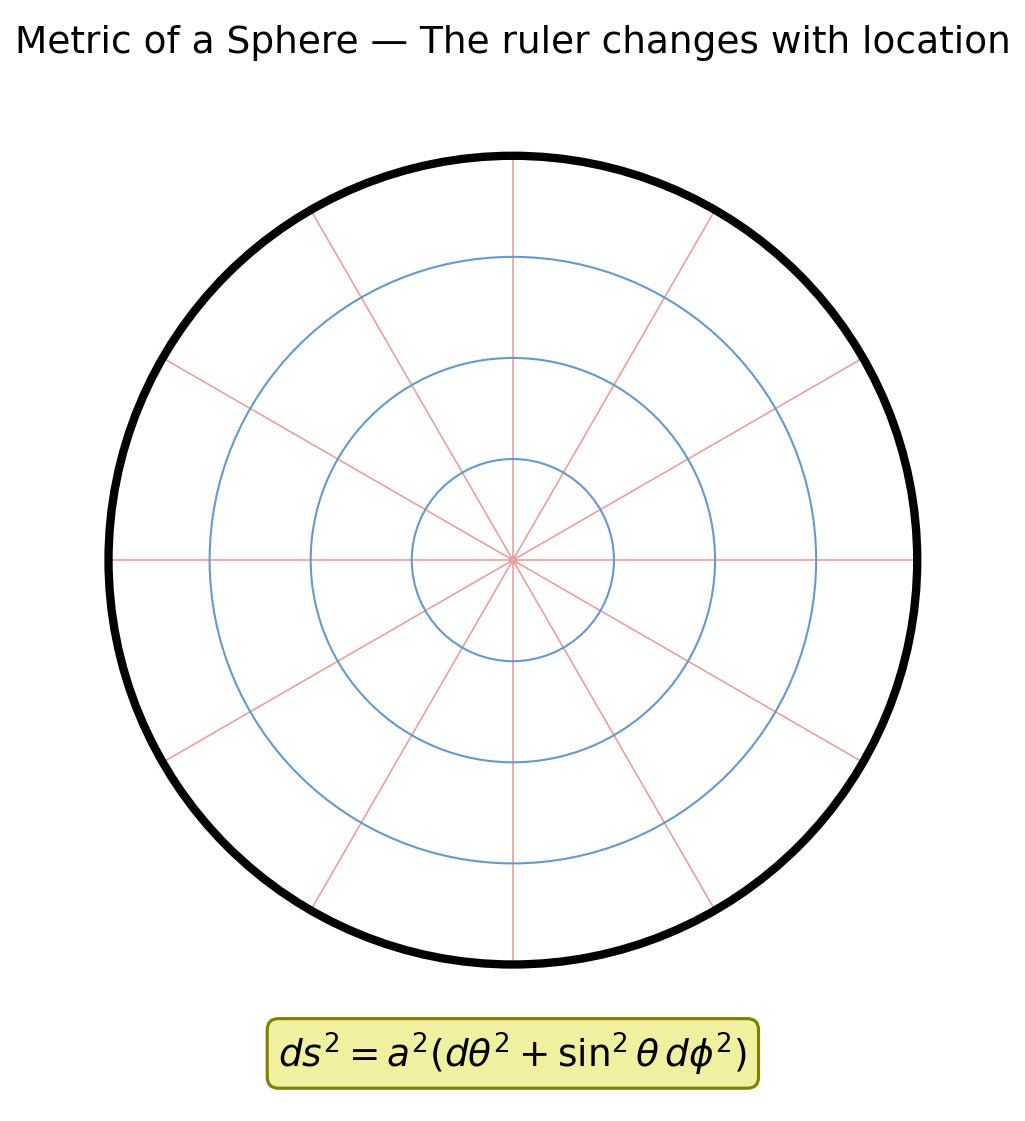
Fig. 6.7: Metric of the sphere and coordinate line spacing. Near the equator, the spacing between meridians (\(\varphi\) = const lines) is wide, while near the poles it narrows. This is the geometric manifestation of \(g_{22} = a^2\sin^2\theta\) depending on \(\theta\).
🟡 Lina: Let me restate the important point from §4 about the sphere's metric, now in the language of coordinate basis vectors.
- Even in flat space, using curvilinear coordinates makes \(g_{ij}\) position-dependent (e.g., \(g_{22} = r^2\) in polar coordinates)—but this can be transformed back to \(\delta_{ij}\). In the language of coordinate basis: "even if the lengths and directions of basis vectors change from place to place, that's just due to the choice of coordinates, and the space itself isn't distorted"
- In genuinely curved space (like a sphere), \(g_{ij}\) cannot be made constant (globally) no matter what coordinates you use. However, in a sufficiently small region—an infinitesimal neighborhood around a single point—coordinates can always be found where \(g_{ij} \approx \delta_{ij}\). This means "even in curved space, if you look at a small enough region, it appears flat"—the same intuition as the Earth's surface appearing locally flat
⚪ Mei: So the sphere's metric can be made \(\delta_{ij}\) in a neighborhood of one point but not globally—that's the meaning of "genuinely curved."
✅ Comprehension Check: When the metric tensor components depend on position, can we say the space is curved?
Answer
No. Even in flat space, using curvilinear coordinates makes the metric tensor position-dependent (e.g., \(g_{22} = r^2\) in polar coordinates). Determining whether space is truly curved requires the Riemann curvature tensor.
6.7 Extension to 4-Dimensional Spacetime¶
🟡 Lina: Finally, let's extend the discussion so far to 4-dimensional spacetime. With coordinates \((x^0, x^1, x^2, x^3)\), the line element is:
Here \(\mu, \nu\) run from 0 to 3. By convention, Greek letters \(\mu, \nu, \ldots\) are used for spacetime indices (0–3), and Latin letters \(i, j, \ldots\) for spatial indices only (1–3). We wrote \(g_{ij}\) in the first half of this chapter because we were only dealing with spatial components; when treating all of 4-dimensional spacetime, we write \(g_{\mu\nu}\). The \(4 \times 4\) symmetric matrix \(g_{\mu\nu}\) has \(\dfrac{4 \times 5}{2} = 10\) independent components.
🔵 Kai: What about in Minkowski spacetime from special relativity?
🟡 Lina: In Cartesian coordinates \((t, x, y, z)\):
So \(g_{\mu\nu} = \mathrm{diag}(-c^2, 1, 1, 1)\). In earlier chapters we used natural units (\(c = 1\)) with coordinates \((ct, x, y, z)\) and wrote \(\eta_{\mu\nu} = \mathrm{diag}(-1, 1, 1, 1)\). In this chapter we've returned to SI units with \(x^0 = t\) (units of seconds), so \(c^2\) appears explicitly. The Minkowski metric's appearance changes depending on the choice of coordinates, but both describe the same flat spacetime, so the essence is the same.
Notation convention: From this chapter onward, the general metric tensor is written \(g_{\mu\nu}\). Minkowski spacetime is also expressed as \(g_{\mu\nu}\) as a special case (the notation \(\eta_{\mu\nu}\) from earlier chapters is used when we want to emphasize that \(g_{\mu\nu}\) is the Minkowski metric).
🔵 Kai: The minus sign is the same sign convention as the Minkowski invariant. But in the previous chapter \(\eta_{00} = -1\), while now \(g_{00} = -c^2\)—the sign is the same but the magnitude changed. Why?
🟡 Lina: Good question. As noted at the beginning of the chapter, here we're taking coordinates \((t, x, y, z)\) (\(x^0 = t\), units of seconds)—a different choice from the \((ct, x, y, z)\) of previous chapters. Since we want the overall dimension of \(ds^2\) to be length squared (m²), and \(dt\) has units of seconds (s), for \(g_{00}\,(dt)^2\) to have units of m², \(g_{00}\) must have units of m²/s²—hence \(g_{00} = -c^2\) (where \(c\) has units of m/s). If you take coordinates \((ct, x, y, z)\), then \(ct\) already has units of m, so you can write \(g_{\mu\nu} = \mathrm{diag}(-1, 1, 1, 1)\) dimensionlessly—that's precisely the \(\eta_{\mu\nu}\) from earlier chapters. In either case, all components are constants, so Minkowski spacetime is flat.
⚪ Mei: Depending on how you choose the units for coordinates, it becomes either \(-1\) or \(-c^2\), but physically it's the same flat spacetime—the same structure as the relationship between polar and Cartesian coordinates.
🔵 Kai: I see, so it becomes either \(-1\) or \(-c^2\) depending on the choice of coordinates, but the essence is the same. And is the minus sign itself related to the causal structure we learned before—the distinction between inside and outside the light cone?
🟡 Lina: Exactly. The minus sign that preserves causal structure appears directly in \(g_{00}\). This means the form of the metric tensor automatically encodes the causal structure of spacetime.
🟡 Lina: Changing to spherical coordinates \((t, r, \theta, \varphi)\):
⚪ Mei: The metric depends on position, but the spacetime itself is flat. We've just changed the choice of coordinates.
Table 6.2: Minkowski spacetime metric: different representations by coordinate choice
| Coordinates | \(g_{\mu\nu}\) | Position dependence | Spacetime curvature |
|---|---|---|---|
| \((ct, x, y, z)\) (previous chapter notation) | \(\eta_{\mu\nu} = \mathrm{diag}(-1, 1, 1, 1)\) | None (constant) | Flat |
| \((t, x, y, z)\) (\(c\) explicit) | \(\mathrm{diag}(-c^2, 1, 1, 1)\) | None (constant) | Flat |
| \((t, r, \theta, \varphi)\) | \(\mathrm{diag}(-c^2, 1, r^2, r^2\sin^2\theta)\) | Yes | Flat |
🟡 Lina: Right. But let me give you a preview of the Schwarzschild metric that will appear in later chapters—the metric describing the spacetime outside a spherically symmetric body of mass \(M\) (such as a black hole). \(G\) is the gravitational constant:
Do you remember the relativistic parameter \(GM/(Rc^2)\) (\(R\) being the radius of the body) that appeared in the Prologue? The \(2GM/(rc^2)\) appearing here uses \(r\) as a coordinate—representing any position outside the body, with \(r = R\) at the body's surface. The meaning of the factor of 2 will become clear in the chapter where we formally introduce the Schwarzschild metric.
🔵 Kai: Wow, compared to the Minkowski metric, \(g_{00}\) and \(g_{11}\) are modified by \(r\)-dependent terms... If the mass \(M\) is zero, it reduces back to Minkowski.
🟡 Lina: Exactly. And this metric cannot globally be transformed to the Minkowski metric by any coordinate transformation. This is what "spacetime is genuinely curved" means.
🔵 Kai: The metric tensor is "a ruler that changes from place to place," and the way that ruler changes contains information about gravity... But looking at the Schwarzschild metric formula, the denominator becomes zero at \(r = 2GM/c^2\). Does that mean the "ruler" gets infinitely stretched there? Or does space actually break down?
🟡 Lina: Sharp question. To state the conclusion first: the divergence at \(r = 2GM/c^2\) is a coordinate singularity—it's merely a poor choice of coordinates, and spacetime itself isn't broken. Using different coordinates, you can pass through smoothly. This is precisely where the distinction between "curvature of coordinates" and "curvature of space" that we learned in this chapter becomes relevant. The tool for determining whether something is a genuine physical singularity or just a coordinate problem is the Riemann curvature tensor. We'll cover this in the chapter where we study the Schwarzschild metric in detail, so look forward to it.
⚪ Mei: The perspective we learned in this chapter—"curvature of coordinates and curvature of space are different"—applies directly there. I can clearly see that the metric tensor is the protagonist of general relativity.
🟡 Lina: Right. All information about the gravitational field is packed into \(g_{\mu\nu}\). In the next chapter, we'll use this metric tensor to actually describe "spacetime with gravity."
Preview of the Next Chapter¶
In Ch. 7, we use the metric tensor \(g_{\mu\nu}\) to actually describe "spacetime with gravity." We'll formally introduce the Schwarzschild metric previewed in this chapter and interpret what each of its components means. From the differences with the Minkowski metric, we'll see how gravitational time dilation and spatial distortion manifest themselves.
Exercises¶
📝 Exercises:
- Jacobian matrix and inverse → Problem B-1. Jacobian of 2D Polar Coordinates, Problem B-5. Jacobian Matrix of a Linear Coordinate Transformation, Problem B-8. Determinant of the Jacobian Matrix of the Inverse Transformation
- Reading metric tensors and inverse metrics → Problem B-2. Inverse Metric in 3D Spherical Coordinates, Problem B-3. Matrix Representation of a General 2-Dimensional Metric, Problem B-4. Metric Tensor on a Sphere at a Specific Point
- Metric tensor transformation law and symmetry → Problem B-6. Application of the Metric Tensor Transformation Law, Problem M-1. Coordinate Transformation \((u, v)\) and the Metric Tensor, Problem M-2. Derivation of the Line Element in Spherical Coordinates, Problem M-3. Metric Tensor in Parabolic Coordinates, Problem M-4. Proof of Symmetry of the Metric Tensor, Problem M-7. Derivation of \(g'_{33}\) using the metric tensor transformation law
- Coordinate basis, curvature of spheres, cylindrical surfaces, Rindler coordinates → Problem B-7. Cartesian Components of Coordinate Basis Vectors, Problem M-5. Metric and Flatness of a Cylindrical Surface, Problem M-6. Geometry of "Circles" on a Sphere, Problem A-1. Metric Tensor in General Curvilinear Coordinates, Problem A-2. Rindler Coordinates
References¶
- 石井俊全『一般相対性理論を一歩一歩数式で理解する』(ベレ出版)第 3 章「テンソルと直線座標のテンソル場」・第 5 章「曲線座標のテンソル場」
- Lancaster, T. & Blundell, S. J., General Relativity for the Gifted Amateur, Ch. 3
- Schutz, B. F., A First Course in General Relativity, 3rd ed., Ch. 6
- Hartle, J. B., Gravity: An Introduction to Einstein's General Relativity, Ch. 2, Ch. 7
- 佐藤勝彦『相対性理論』(岩波基礎物理シリーズ)第 4 章「リーマン幾何学」
Feedback on this page
Let us know if something was unclear, incorrect, or could be improved.