Appendix D: Lagrangian/Hamiltonian Formalism and Canonical Quantization
Story so far:
In the main text, Chapters 1–28, we built the complete picture of quantum mechanics starting from probability amplitudes. In Appendix A through C, we developed the mathematical tools of complex numbers, linear algebra, and Fourier analysis. In this Appendix D, we systematically introduce the Lagrangian and Hamiltonian formalisms of classical mechanics, and make explicit the translation procedure from classical mechanics to quantum mechanics—canonical quantization.
Goals of this chapter
- Systematically understand the Lagrangian and Hamiltonian formalisms of classical mechanics, and recognize that the algebraic structure of Poisson brackets is isomorphic to that of quantum mechanical commutation relations
- On that basis, clearly grasp the "recipe" of canonical quantization—replacing the Poisson bracket \(\{q_j, p_k\} = \delta_{jk}\) with the commutation relation \([\hat{q}_j, \hat{p}_k] = i\hbar\,\delta_{jk}\)—and trace the origin of the Hamiltonian operator and Schrödinger equation, which were introduced "from above" in the main text, all the way back to classical mechanics
- Furthermore, survey the natural extension to canonical quantization of fields, gaining a perspective toward quantum field theory
D.1 Why We Need the Lagrangian Formalism
🟡 Lina: Now, in the main text we built quantum mechanics from the "rules of probability amplitudes." But from Ch. 7 onward, when we used the Schrödinger equation, the Hamiltonian \(\hat{H}\) suddenly appeared, right? Understanding where that \(\hat{H}\) comes from—tracing its origin back to classical mechanics—is the purpose of this Appendix.
🔵 Kai: Isn't Newton's \(F = ma\) enough?
🟡 Lina: Good question. Newton's equation of motion takes "force" as the fundamental concept. But in quantum mechanics, the very notion of "which path a particle takes" becomes uncertain. Recall Feynman's path integral from Ch. 4—there we said "assign a probability amplitude \(e^{iS/\hbar}\) to every path."
🔵 Kai: Ah, that \(S\) is...
🟡 Lina: Yes, the action. The action \(S\) is defined as the time integral of the Lagrangian \(L\). In other words, the Lagrangian sits at the very heart of quantum mechanics. Not Newton's "force" but the Lagrangian's "action" serves as the bridge connecting classical and quantum mechanics. And going further from the Lagrangian to the Hamiltonian formalism makes the translation to quantum mechanics possible. So the progression has been: Newton's formalism → Lagrangian formalism → Hamiltonian formalism → quantum mechanics.
⚪ Mei: I see—at each stage the level of abstraction increases, and ultimately the connection to quantum mechanics becomes possible.
🟡 Lina: Exactly. Let me list the specific advantages of the Lagrangian formalism:
- Coordinate-independent — The Euler-Lagrange equations take the same form in any coordinate system
- Easy handling of constraints — Properly choosing degrees of freedom handles them naturally
- Symmetries directly connect to conservation laws — Noether's theorem, which we learned in Ch. 26
- Extends to fields — Can be used uniformly for electromagnetic fields and quantum fields
- Direct bridge to quantum theory — Feynman's path integral uses the weight \(e^{iS/\hbar}\)
🔵 Kai: Number 5 seems the most important.
🟡 Lina: Indeed. Now let's begin concretely with the principle of least action.
✅ Comprehension Check: What is the primary reason the Lagrangian formalism is better suited than Newton's formalism for connecting to quantum mechanics?
Answer
In Feynman's path integral, the phase of the probability amplitude assigned to each path, \(e^{iS/\hbar}\), is written in terms of the action \(S\), which is the time integral of the Lagrangian. In other words, the Lagrangian (action) sits directly at the heart of quantum mechanics, and it is the Lagrangian's "action"—not Newton's "force"—that serves as the bridge connecting classical and quantum mechanics.
D.2 The Action and the Principle of Least Action
🟡 Lina: Consider a particle of mass \(m\) moving in one dimension. Let the position be \(q(t)\) and the velocity be \(\dot{q}(t) = dq/dt\). The Lagrangian \(L\) is defined as follows:
Here \(T\) is the kinetic energy and \(V\) is the potential energy.
🔵 Kai: It's \(T - V\) instead of the total energy \(E = T + V\)? Subtraction?
🟡 Lina: Yes. Intuitively, it's a weighting where "more kinetic energy is favorable, more potential energy is unfavorable." As for why it's subtraction, ultimately we can only say "because the correct equations of motion emerge from this definition." The justification of the model comes from agreement with experiment.
🟡 Lina: The action \(S\) is obtained by integrating this Lagrangian over time:
⚪ Mei: The square brackets in \(S[q]\) mean...
🟡 Lina: Good catch. \(S\) is a functional. An ordinary function takes "a number in and gives a number out," but a functional takes "a function in and gives a number out." It takes the entire path \(q(t)\) as a function as input and returns a single real number \(S\). That's why we write \(S[q]\) with square brackets to distinguish it from an ordinary function \(f(x)\) with parentheses (those who have studied General Relativity will recognize this as the same concept from General Relativity Ch. 1). A familiar example: "the length of a curve" is also a functional—it takes the shape of a curve (a function) as input and returns its length (a number), right?
🔵 Kai: I see... each path gets a numerical value called the "action."
🟡 Lina: Right. And the principle of least action states:
When a particle is at position \(q(t_1) = q_A\) at time \(t_1\) and at position \(q(t_2) = q_B\) at time \(t_2\), the path actually followed is the one that makes the action \(S[q]\) stationary.
🔵 Kai: Is "stationary" different from "minimum"?
🟡 Lina: Strictly speaking, it's not necessarily a "minimum"—it's "stationary," meaning the first-order change in \(S\) vanishes under infinitesimal path variations. Just as with ordinary functions where a point with "derivative = 0" could be a maximum, minimum, or saddle point, a stationary point isn't necessarily a minimum. But historically it's called the "principle of least action."
⚪ Mei: So among all "possible paths," only the special path where the action is stationary is physically realized.
🟡 Lina: Exactly. Here an important question arises—"Why does nature choose the path that makes the action stationary?" The answer is actually provided by quantum mechanics.
🔵 Kai: Wait, quantum mechanics?
🟡 Lina: In Feynman's path integral, the particle travels all paths simultaneously. Each path is assigned a phase factor \(e^{iS/\hbar}\). In the classical limit (\(\hbar \to 0\)), only the neighborhood of the path where the action is stationary produces constructive interference—all other paths oscillate wildly and cancel out. So classically, it appears that "only the stationary path survives."
🔵 Kai: Amazing... quantum mechanics answers the "why" of classical mechanics. So conversely, if we lived in a purely classical world, we could never answer "why the action is stationary"?
🟡 Lina: Exactly. Within the framework of classical mechanics alone, the principle of least action must simply be accepted as a "principle." But quantum mechanics reveals the underlying mechanism—a deeper theory answers the "why" of a shallower theory. Now, today's goal is first to derive the equations of motion from the "stationarity condition" within the framework of classical mechanics. We'll do that in the next section.
✅ Comprehension Check: In the classical limit (\(\hbar \to 0\)), explain how the principle of least action is derived from Feynman's path integral.
Answer
In the path integral, each path is assigned a phase factor \(e^{iS/\hbar}\). In the limit \(\hbar \to 0\), near paths where the action is not stationary, the phase oscillates rapidly and the contributions cancel each other out (destructive interference). On the other hand, near the path where the action is stationary, the phase varies slowly and constructive interference occurs. As a result, classically only the stationary path survives.
✅ Comprehension Check: State in one sentence why the action \(S[q]\) is called a "functional."
Answer
Because the action \(S\) takes a "function"—the path \(q(t)\)—as input and returns a single real number. While an ordinary function is a "number → number" mapping, a functional is a "function → number" mapping.
D.3 Derivation of the Euler-Lagrange Equation
🟡 Lina: Let's derive the equation of motion from the principle of least action. Taking the actual path as \(q(t)\), consider a path slightly displaced from it, \(q(t) + \delta q(t)\). The endpoints are fixed:
🔵 Kai: So the starting and ending points don't move.
🟡 Lina: Right. Let's compute the variation of the action \(\delta S\):
Taylor expanding \(L\) to first order in \(\delta q\) and \(\delta\dot{q}\):
⚪ Mei: This is the first-order Taylor expansion of a two-variable function. Same structure as \(f(x+\Delta x, y+\Delta y) \approx f(x,y) + \frac{\partial f}{\partial x}\Delta x + \frac{\partial f}{\partial y}\Delta y\).
🟡 Lina: Exactly. Substituting this into equation (D.4):
Since \(\delta\dot{q} = \frac{d}{dt}(\delta q)\), we integrate by parts on the second term:
🔵 Kai: Integration by parts is \(\int u\,dv = uv - \int v\,du\), right?
🟡 Lina: Yes. And the boundary term \(\left[\frac{\partial L}{\partial \dot{q}}\,\delta q\right]_{t_1}^{t_2}\) vanishes due to the endpoint conditions \(\delta q(t_1) = \delta q(t_2) = 0\). Therefore:
🔵 Kai: Everything up to here is mechanical calculation. But now we use "\(\delta S = 0\)" to extract the equation of motion, right?
🟡 Lina: Exactly. The stationarity condition is "\(\delta S = 0\) for arbitrary \(\delta q(t)\)." Here "arbitrary" means that as long as \(\delta q(t_1) = \delta q(t_2) = 0\) is satisfied at the endpoints, any smooth function in the interior of the interval will do. For the integral of the integrand multiplied by any such function \(\delta q\) to be zero, the integrand itself must be zero. This is called the fundamental lemma of the calculus of variations. Mathematically: "If \(\int f(t)\,\delta q(t)\,dt = 0\) for all \(\delta q\) vanishing at the endpoints, then \(f(t) = 0\)." Intuitively, if the integrand \(f(t)\) were nonzero somewhere, you could choose a \(\delta q\) that is positive only near that point and make the integral nonzero—so \(f(t) = 0\) must hold.
⚪ Mei: I see—the condition "the integral is zero for arbitrary \(\delta q\)" forces the integrand itself to be zero.
🟡 Lina: Exactly. This gives us the Euler-Lagrange equation:
🔵 Kai: Does this replace Newton's \(F = ma\)?
🟡 Lina: Let's verify. Substituting \(L = \frac{1}{2}m\dot{q}^2 - V(q)\):
Putting these into the Euler-Lagrange equation:
🔵 Kai: Oh, it's Newton's second law itself!
⚪ Mei: So the Euler-Lagrange equation contains Newton's equation of motion but is a more general formalism. The form of equation (D.9) doesn't change when you switch coordinate systems.
🟡 Lina: Right. For a multi-degree-of-freedom system \(q_1, q_2, \ldots, q_f\), there's one equation for each degree of freedom:
✅ Comprehension Check: What is the fundamental lemma of the calculus of variations? How is it used in deriving the Euler-Lagrange equation?
Answer
The fundamental lemma of the calculus of variations states: "If \(\int f(t)\,\delta q(t)\,dt = 0\) for all functions \(\delta q(t)\), then \(f(t) = 0\)." In deriving the Euler-Lagrange equation, from the fact that \(\delta S = \int \left(\frac{\partial L}{\partial q} - \frac{d}{dt}\frac{\partial L}{\partial \dot{q}}\right)\delta q\,dt = 0\) holds for arbitrary \(\delta q\), we conclude the integrand itself is zero, which gives the Euler-Lagrange equation.
✅ Comprehension Check: In deriving the Euler-Lagrange equation, why does the boundary term from integration by parts vanish?
Answer
Because we impose the condition of fixed endpoints \(\delta q(t_1) = \delta q(t_2) = 0\). Since the variation \(\delta q\) is zero at both endpoints, the boundary term \(\left[\frac{\partial L}{\partial \dot{q}}\,\delta q\right]_{t_1}^{t_2} = 0\).
📝 Exercises:
- Derive the Euler-Lagrange equations from the Lagrangian in 2D polar coordinates → Problem M-1. Derivation of Euler-Lagrange Equations in 2D Polar Coordinates
D.4 Canonical Momentum and the Legendre Transform
🟡 Lina: The Euler-Lagrange equation is a second-order differential equation. The variables are \(q\) and \(\dot{q}\). But in quantum mechanics, we want to treat "position" and "momentum" on equal footing. So we perform an operation that replaces the independent variable \(\dot{q}\) with a different quantity.
D.4.1 Definition of Canonical Momentum
🟡 Lina: We define the canonical momentum as:
🔵 Kai: For \(L = \frac{1}{2}m\dot{q}^2 - V(q)\), we get \(p = m\dot{q}\), which is just the ordinary momentum, right?
🟡 Lina: In that case, yes. But in general, it's not necessarily "mass × velocity." For example, for a charged particle in an electromagnetic field, \(p = m\dot{q} + eA\) (where \(A\) is the vector potential), so the field contributes. The canonical momentum is a quantity determined automatically from the structure of the Lagrangian, and it can differ from the everyday intuition of "momentum"—this is an important point.
✅ Comprehension Check: Give an example where the canonical momentum does not equal "mass × velocity," and explain why this happens.
Answer
For a charged particle in an electromagnetic field, the canonical momentum is \(p = m\dot{q} + eA\), which includes a contribution from the vector potential \(A\). This happens because the canonical momentum is defined as \(p = \frac{\partial L}{\partial \dot{q}}\), determined automatically from the structure of the Lagrangian, and when the Lagrangian contains coupling terms between velocity and the field (such as \(e\dot{q}A\)), it differs from simple "mass × velocity."
D.4.2 Motivation for the Legendre Transform
🟡 Lina: The Lagrangian \(L(q, \dot{q})\) is a function of \(q\) and \(\dot{q}\). But to proceed to quantum mechanics, we want a new function with \(q\) and \(p\) as independent variables. In mathematics, this "change of independent variable" is called the Legendre transform.
🔵 Kai: Why do we want to change variables?
🟡 Lina: There are two reasons. First, treating \(q\) and \(p\) on equal footing makes the structure of mechanics more symmetric and elegant. Second, since \(\hat{q}\) and \(\hat{p}\) are the fundamental operators in quantum mechanics, describing classical mechanics in terms of \(q\) and \(p\) makes the transition to quantization natural.
🟡 Lina: Let me explain the general idea of the Legendre transform. Given a function \(f(x)\):
- Define a new variable \(s = \frac{df}{dx}\)
- Define a new function \(g(s) = sx - f(x)\) (eliminating \(x\) as a function of \(s\))
This is the Legendre transform. The information in the original function \(f\) is completely preserved in \(g\), and you can recover \(f\) by an inverse transform.
🔵 Kai: Why is the information preserved? You mean you can get \(f\) back from \(g\)?
🟡 Lina: Yes. Let's verify the inverse transform. To show that "\(f\) can be recovered from \(g\)," let's differentiate \(g(s)\) with respect to \(s\). Why differentiate? Because in the definition of the Legendre transform we "differentiated \(f\) to create the new variable \(s\)," so conversely, "differentiating \(g\) should recover the original variable \(x\)"—we're expecting a symmetric structure.
🟡 Lina: What's important here is that the relation \(s = \frac{df}{dx}\) can be solved in reverse to determine \(x\) as a function of \(s\)—that is, we can write \(x = x(s)\). "Solving in reverse" means, for example, if \(f(x) = x^2\) then \(s = f'(x) = 2x\) so \(x = s/2\). In other words, "once the value of \(s\) is determined, exactly one corresponding \(x\) is determined."
🔵 Kai: Can you always solve it in reverse?
🟡 Lina: Good question. To solve \(s = f'(x)\) for \(x\), we need \(f'(x)\) to be a monotonic function—either always increasing or always decreasing. If it's monotonic, then "specifying one value of \(s\) determines exactly one corresponding \(x\)," so the inverse function exists. What's the condition for \(f'\) to be monotonic? Recall that \(f''(x)\) is the derivative of \(f'(x)\) with respect to \(x\)—it represents "the slope of the graph of \(f'\)." If \(f'' > 0\) always holds, the graph of \(f'\) always slopes upward (monotonically increasing); if \(f'' < 0\) always holds, it always slopes downward (monotonically decreasing)—in either case it never turns back. In short, the condition is "\(f''\) always maintains the same sign."
⚪ Mei: So "the Legendre transform is well-defined for convex functions."
🟡 Lina: Exactly. Conversely, if \(f\) is linear (\(f'' = 0\) everywhere), then \(s = f'(x)\) becomes a constant, giving the same \(s\) for every \(x\), so it can't be inverted. The Lagrangians encountered in physics usually satisfy this condition. For example, with \(L = \frac{1}{2}m\dot{q}^2 - V(q)\), viewing \(L\) as a function of \(\dot{q}\) (with \(q\) held fixed), differentiating twice with respect to \(\dot{q}\) gives \(\frac{\partial^2 L}{\partial \dot{q}^2} = m > 0\)—this corresponds to the \(f''(x) > 0\) condition above. So \(p = \frac{\partial L}{\partial \dot{q}} = m\dot{q}\) is a monotonically increasing function of \(\dot{q}\), and solving inversely gives \(\dot{q} = p/m\) uniquely.
Now, assuming the condition is satisfied, let's actually compute \(\frac{dg}{ds}\).
🔵 Kai: The right side has both \(x\) and \(f(x)\), and both change through \(s\), right? If we shift \(s\) slightly, \(x\) moves accordingly, so when differentiating \(sx\) we need to pick up the change in \(x\) too?
🟡 Lina: Exactly. Since \(x\) is a function of \(s\)—the \(x(s)\) obtained by inverting \(s = f'(x)\)—when differentiating with respect to \(s\), we need to account for the change in \(x\) as well. We use the product rule and the chain rule. Let me work through it carefully. Differentiating the first term \(sx\) with respect to \(s\) using the product rule \((uv)' = u'v + uv'\) gives \(1 \cdot x + s \cdot \frac{dx}{ds} = x + s\frac{dx}{ds}\). Differentiating the second term \(-f(x)\) with respect to \(s\) using the chain rule gives \(-\frac{df}{dx}\cdot\frac{dx}{ds}\). Combining:
🟡 Lina: Now recall that \(s = \frac{df}{dx}\). Substituting \(\frac{df}{dx} = s\) into the third term \(-\frac{df}{dx}\frac{dx}{ds}\) gives \(-s\frac{dx}{ds}\). This has the opposite sign and same magnitude as the second term \(+s\frac{dx}{ds}\), so they cancel completely! That is:
🔵 Kai: Oh, it cancels beautifully!
⚪ Mei: So \(\frac{dg}{ds} = x\). Just differentiating \(g\) recovers the original variable \(x\).
🟡 Lina: Right. So the inverse transform is "define a new variable \(x = \frac{dg}{ds}\) from \(g(s)\), and recover \(f(x) = xs - g(s)\)"—exactly the same structure as the original transform. The Legendre transform is a symmetric operation that "returns to the original when applied twice."
🔵 Kai: What does this look like concretely?
🟡 Lina: Let's do a simple example. If \(f(x) = x^2\), then \(s = \frac{df}{dx} = 2x\) so \(x = s/2\). The new function is \(g(s) = sx - f(x) = s \cdot \frac{s}{2} - \left(\frac{s}{2}\right)^2 = \frac{s^2}{4}\). The independent variable has been switched from \(x\) to \(s\). Conversely, from \(g(s) = \frac{s^2}{4}\) we recover \(\frac{dg}{ds} = \frac{s}{2} = x\), and \(f = xs - g(s) = \frac{s}{2}\cdot s - \frac{s^2}{4} = \frac{s^2}{4} = x^2\), returning to the original.
D.4.3 Definition of the Hamiltonian
🟡 Lina: Let's apply the Legendre transform to the Lagrangian. For \(L(q, \dot{q})\):
- New variable: \(p = \frac{\partial L}{\partial \dot{q}}\) (canonical momentum)
- New function: the Hamiltonian \(H\)
Here \(\dot{q}_j\) is expressed as a function of \(q\) and \(p\) by inverting \(p_j = \frac{\partial L}{\partial \dot{q}_j}\). By the way, in physics there's a notational convention that "when the same index appears twice, summation over that index is implied automatically"—this is called the Einstein summation convention. So writing \(p_j\dot{q}_j\) alone means \(\sum_j p_j\dot{q}_j = p_1\dot{q}_1 + p_2\dot{q}_2 + \cdots + p_f\dot{q}_f\). In this Appendix I'll often write \(\sum\) explicitly for clarity, so treat both notations as meaning the same thing.
🔵 Kai: What does \(H\) represent?
🟡 Lina: In many cases, it corresponds to the system's total energy. Let's verify. For \(L = \frac{1}{2}m\dot{q}^2 - V(q)\), we have \(p = m\dot{q}\) so \(\dot{q} = p/m\). Substituting:
⚪ Mei: \(T + V\)—the sum of kinetic and potential energy. The Lagrangian was \(T - V\), while the Hamiltonian is \(T + V\).
🟡 Lina: Right. But be careful—the Hamiltonian doesn't always equal the energy. It can differ depending on the choice of coordinates or when the Lagrangian explicitly depends on time. But within the scope of this Appendix, you can safely think of \(H = E\).
✅ Comprehension Check: State the purpose of the Legendre transform in one sentence.
Answer
To replace the independent variable from \(\dot{q}\) (generalized velocity) to \(p\) (canonical momentum). This allows \(q\) and \(p\) to be treated as equal independent variables, making the transition to quantization natural.
D.5 Hamilton's Equations of Motion
🟡 Lina: From the Hamiltonian \(H(q, p)\), equations of motion in a different form from the Euler-Lagrange equations can be derived. These are Hamilton's equations of motion (canonical equations).
D.5.1 Derivation
🟡 Lina: Let's consider the infinitesimal change of the right side of \(H = \sum_j p_j\dot{q}_j - L\) (here I'll write \(\sum_j\) explicitly). The key point is that while three types of quantities appear on the right side—\(q_j\), \(\dot{q}_j\), \(p_j\)—the definition of \(p_j\) as \(p_j = \frac{\partial L}{\partial \dot{q}_j}\) means \(\dot{q}_j\) is determined as a function of \((q, p)\). But first, let's formally vary \(q_j\), \(\dot{q}_j\), and \(p_j\) all independently.
🔵 Kai: Wait, we can vary them independently even though there's a dependency relation?
🟡 Lina: Good question. The approach is this—first "formally compute what \(\delta H\) would be if \(q\), \(\dot{q}\), \(p\) were all independent." The strategy is "compute assuming independence, and if no contradiction arises, we're fine." In fact, when we compute, the coefficient of \(\delta\dot{q}\) turns out to be zero. This serves as a proof that "\(H\) doesn't actually depend on \(\dot{q}\)."
🔵 Kai: So you're saying that "we assume independence for the calculation, and as a result the \(\dot{q}\) term vanishes. Therefore we learn after the fact that \(H\) doesn't depend on \(\dot{q}\)"?
🟡 Lina: Exactly! We're not "assuming" that they're independent—rather, by varying independently and computing, the absence of dependence on \(\dot{q}\) is "derived" as a result. This is precisely the power of the Legendre transform: the evidence that "we chose the correct set of variables \((q, p)\)" manifests as the vanishing of the \(\delta\dot{q}\) term.
🔵 Kai: Hmm, I understand in words, but how does it actually cancel?
🟡 Lina: Good question. Let me first show a simple 1-degree-of-freedom example to build intuition, then do the general case. For \(L = \frac{1}{2}m\dot{q}^2 - V(q)\), we have \(p = m\dot{q}\), and \(H = p\dot{q} - L = m\dot{q}\cdot\dot{q} - \frac{1}{2}m\dot{q}^2 + V(q) = \frac{1}{2}m\dot{q}^2 + V(q)\). Substituting \(\dot{q} = p/m\) gives \(H = \frac{p^2}{2m} + V(q)\)—indeed \(\dot{q}\) has disappeared and it's a function of \((q, p)\) only. Now I'll show that this happens in the general case too.
🟡 Lina: Let's proceed to the general calculation. We vary the \(\sum_j p_j\dot{q}_j\) part. The same product rule that works for derivatives works for variations—\(\delta(AB) = A\,\delta B + B\,\delta A\). Applying this to each term \(p_j\dot{q}_j\) gives \(\delta(p_j\dot{q}_j) = \dot{q}_j\,\delta p_j + p_j\,\delta\dot{q}_j\), so overall \(\delta(\sum_j p_j\dot{q}_j) = \sum_j(\dot{q}_j\,\delta p_j + p_j\,\delta\dot{q}_j)\). Next, for the \(L(q, \dot{q})\) part, the first-order Taylor expansion gives \(\delta L = \sum_j\left(\frac{\partial L}{\partial q_j}\delta q_j + \frac{\partial L}{\partial \dot{q}_j}\delta\dot{q}_j\right)\). Combining:
🔵 Kai: There are four terms, and I should focus on the coefficient of \(\delta\dot{q}\).
🟡 Lina: Exactly. Since \(p_j = \frac{\partial L}{\partial \dot{q}_j}\), the second term \(p_j\,\delta\dot{q}_j\) and the fourth term \(-\frac{\partial L}{\partial \dot{q}_j}\delta\dot{q}_j\) cancel completely!
🔵 Kai: Wait, they cancel? But why do they conveniently cancel?
🟡 Lina: Good question. This isn't coincidence—it's an essential property of the Legendre transform. Precisely because we defined \(p_j\) as \(\frac{\partial L}{\partial \dot{q}_j}\), the \(\delta\dot{q}\) terms cancel. And the cancellation means that the change in \(H\) can be written using only \(\delta q\) and \(\delta p\)—confirming that \(H\) is self-contained as a function of \((q, p)\) alone and doesn't contain \(\dot{q}\) as an independent variable.
🔵 Kai: Ah, I see—because we defined \(p\) as "the slope of \(L\) with respect to \(\dot{q}\)," when we switch variables from \(\dot{q}\) to \(p\), it's natural that traces of \(\dot{q}\) disappear.
⚪ Mei: In other words, the evidence that the Legendre transform is "functioning correctly" appears as the vanishing of the \(\delta\dot{q}\) term—\(H\) is confirmed to be a function of \((q, p)\) only.
🟡 Lina: Exactly. What remains is:
On the other hand, since \(H\) is a function of \(q\) and \(p\), in general:
Equations (D.16) and (D.17) both represent the same \(\delta H\), so they must be equal. Since \(q_j\) and \(p_j\) are independent variables of the Hamiltonian—meaning changing one doesn't change the other—\(\delta q_j\) and \(\delta p_j\) can each be chosen freely (just as in the total differential \(df = \frac{\partial f}{\partial x}dx + \frac{\partial f}{\partial y}dy\) of \(f(x, y)\), where \(dx\) and \(dy\) can be chosen independently). For example, making only \(\delta p_1\) nonzero and setting all other \(\delta q_j\), \(\delta p_j\) to zero, both sides become \(\dot{q}_1\,\delta p_1 = \frac{\partial H}{\partial p_1}\delta p_1\), and dividing by \(\delta p_1 \neq 0\) gives \(\dot{q}_1 = \frac{\partial H}{\partial p_1}\). Repeating for all \(j\), each coefficient must match.
⚪ Mei: In Section D.3, from "multiplying by an arbitrary function inside an integral and getting zero" we used the fundamental lemma to deduce that the integrand is zero. Here, without integration, we're "choosing independent variations one at a time" to read off the coefficients. The method differs, but the spirit of "determining coefficients from arbitrariness" is the same.
🟡 Lina: Nice summary. What we obtain is:
🟡 Lina: Note that equation (D.18) \(\dot{q}_j = \frac{\partial H}{\partial p_j}\) comes purely from the structure of the Legendre transform—we haven't used the Euler-Lagrange equation. On the other hand, to rewrite \(\frac{\partial L}{\partial q_j}\) in equation (D.19) as \(\dot{p}_j\), we need the Euler-Lagrange equation (D.9). Rearranging gives \(\frac{\partial L}{\partial q_j} = \frac{d}{dt}\frac{\partial L}{\partial \dot{q}_j}\). The right side is the time derivative of both sides of the canonical momentum definition \(p_j = \frac{\partial L}{\partial \dot{q}_j}\)—that is, \(\frac{d}{dt}\frac{\partial L}{\partial \dot{q}_j} = \frac{dp_j}{dt} = \dot{p}_j\). Therefore equation (D.19) becomes:
Summarizing:
These are Hamilton's canonical equations. Hamilton's equations are equivalent to the Euler-Lagrange equations—the same physics written in a different language.
D.5.2 Comparison of Structures
🟡 Lina: Let's compare the two formalisms here. The Euler-Lagrange equation gives one second-order ordinary differential equation per degree of freedom. Hamilton's equations give two first-order ordinary differential equations per degree of freedom. Mathematically they contain the same information.
⚪ Mei: I see—since one second-order equation is decomposed into two first-order equations, the information content doesn't change.
🟡 Lina: Exactly. And the first-order equations have the symmetry of treating \(q\) and \(p\) on equal footing. The space spanned by \(q\) and \(p\) is called phase space. The phase space of a system with \(f\) degrees of freedom is \(2f\)-dimensional. The state of the system is represented as a single point in phase space, and time evolution is depicted as a trajectory in phase space.
✅ Comprehension Check: What is the dimensionality of the phase space for a system with \(f\) degrees of freedom? How is the state of the system represented in phase space?
Answer
Phase space is \(2f\)-dimensional (spanned by \(f\) generalized coordinates \(q_j\) and \(f\) canonical momenta \(p_j\)). The state of the system is represented as a single point \((q_1, \ldots, q_f, p_1, \ldots, p_f)\) in phase space, and time evolution is depicted as a trajectory (curve) in that space.
D.5.3 Concrete Example: 1D Harmonic Oscillator
🟡 Lina: Let's verify with the one-dimensional harmonic oscillator.
Hamilton's equations:
🔵 Kai: The first equation is \(p = m\dot{q}\) (definition of momentum), and the second is \(m\ddot{q} = -m\omega^2 q\) (spring restoring force). Same as Newton's equation of motion.
🟡 Lina: Right. We're just describing the same physics in a different language. But this Hamiltonian language opens the path to quantization. In phase space \((q, p)\) (Fig. D.1 "Trajectories in the phase space \((q, p)\) of the harmonic oscillator"), energy conservation \(H = E\) means \(\frac{p^2}{2m} + \frac{1}{2}m\omega^2 q^2 = E\)—this is the equation of an ellipse with respect to the \(p\) and \(q\) axes (in the form \(\frac{x^2}{a^2} + \frac{y^2}{b^2} = 1\)). So the trajectories of the harmonic oscillator are closed ellipses corresponding to each energy. Furthermore, Hamilton's equations (D.23)–(D.24) assign a velocity vector to each point \((q, p)\) in phase space telling it "which direction to move next"—this is the "flow" in phase space. Since different energies correspond to ellipses of different sizes, the elliptical orbits nest inside each other for different energies—you can confirm this visually in Fig. D.1 "Trajectories in the phase space \((q, p)\) of the harmonic oscillator".
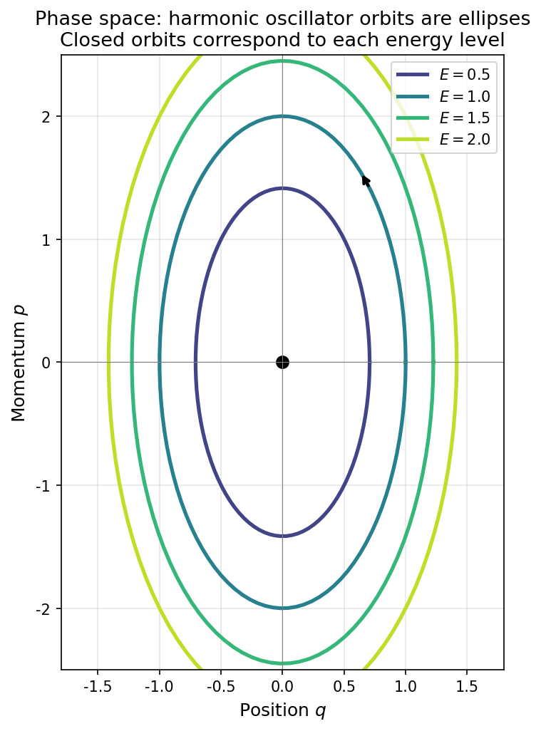
Fig. D.1: Trajectories in the phase space \((q, p)\) of the harmonic oscillator. They appear as closed elliptical orbits corresponding to each energy level. Hamilton's equations (D.23)–(D.24) determine the flow in phase space.
D.5.4 Energy Conservation
🟡 Lina: One more important point. In general, \(H\) is a function of \(q_j(t)\), \(p_j(t)\), and possibly \(t\) itself. To find the time variation of \(H\), we need to consider both "the change due to \(q_j\) and \(p_j\) evolving with time" and "the change due to the functional form of \(H\) itself changing with time."
🔵 Kai: How do those two differences specifically show up in the calculation?
🟡 Lina: First recall the chain rule for a single-variable composite function. The time derivative of \(f(x(t))\) is \(\frac{df}{dt} = \frac{df}{dx}\cdot\frac{dx}{dt}\). If \(f\) has two variables \(f(x(t), y(t))\), you add the contribution from the change in \(x\) and the contribution from the change in \(y\): \(\frac{df}{dt} = \frac{\partial f}{\partial x}\frac{dx}{dt} + \frac{\partial f}{\partial y}\frac{dy}{dt}\). The same pattern holds for any number of variables—just add up "partial derivative of \(f\) with respect to that variable × time rate of change of that variable" for each variable.
Furthermore, if \(f\) depends directly on \(t\) itself in addition to \(x\) and \(y\)—\(f(x(t), y(t), t)\)—then the contribution from the change of \(t\) itself, \(\frac{\partial f}{\partial t}\), also appears. Note the difference between \(\frac{\partial f}{\partial t}\) and \(\frac{df}{dt}\) here. \(\frac{\partial f}{\partial t}\) is "the rate of change when \(x\) and \(y\) are held fixed and only the \(t\) appearing explicitly in \(f\)'s formula is varied." On the other hand, \(\frac{df}{dt}\) is "the total time rate of change of \(f\) including the motion of \(x(t)\) and \(y(t)\) along the actual trajectory."
🔵 Kai: Ah, the difference between partial and total derivatives. \(\frac{\partial}{\partial t}\) means "hold everything else fixed and move only \(t\)," while \(\frac{d}{dt}\) means "move everything together."
🟡 Lina: Exactly. For \(H(q_1, \ldots, q_f, p_1, \ldots, p_f, t)\):
This is the total time derivative formula for a multivariable function (the multivariable version of the chain rule). The first term \(\frac{\partial H}{\partial t}\) represents "the rate of change when \(q_j\) and \(p_j\) are held fixed and only the \(t\) appearing explicitly in \(H\)'s formula is varied"—in other words, it captures whether "the functional form of \(H\) itself changes with time." For a system where external forces change with time, \(\frac{\partial H}{\partial t} \neq 0\), but for an isolated system it's usually zero.
🟡 Lina: When \(H\) does not explicitly depend on time (\(\frac{\partial H}{\partial t} = 0\))—meaning the rules of the system themselves don't change with time—the first term in equation (D.25) is zero. Substituting Hamilton's equations \(\dot{q}_j = \frac{\partial H}{\partial p_j}\), \(\dot{p}_j = -\frac{\partial H}{\partial q_j}\) into the remaining terms:
🔵 Kai: Oh, they cancel completely! The same form appears with opposite signs, so it's zero.
⚪ Mei: So \(\frac{dH}{dt} = 0\), meaning \(H\) is a conserved quantity—energy conservation.
✅ Comprehension Check: In the process of deriving \(\frac{dH}{dt} = 0\) from Hamilton's canonical equations, explain why the two terms cancel.
Answer
Substituting Hamilton's equations \(\dot{q}_j = \frac{\partial H}{\partial p_j}\), \(\dot{p}_j = -\frac{\partial H}{\partial q_j}\) into \(\frac{dH}{dt} = \frac{\partial H}{\partial q_j}\dot{q}_j + \frac{\partial H}{\partial p_j}\dot{p}_j\) gives \(\frac{\partial H}{\partial q_j}\frac{\partial H}{\partial p_j} - \frac{\partial H}{\partial p_j}\frac{\partial H}{\partial q_j} = 0\). The positive and negative terms have exactly the same magnitude but opposite signs, so they cancel.
📝 Exercises:
- Write the Hamiltonian for a 2D central force \(V(r)\) in polar coordinates and derive Hamilton's equations → Problem B-2. Construction of the Hamiltonian via Legendre Transform
D.6 Poisson Brackets — The Algebraic Structure of Classical Mechanics
🟡 Lina: To understand the symmetric structure of Hamilton's equations more deeply, let's introduce a tool called the Poisson bracket. This will be the core of the "translation dictionary" connecting classical and quantum mechanics.
D.6.1 Definition
🟡 Lina: For two physical quantities on phase space—that is, quantities that can be written as functions of \(q\) and \(p\)—\(A(q, p)\) and \(B(q, p)\), the Poisson bracket is defined as:
🔵 Kai: What does it mean? It just looks like a formula...
🟡 Lina: Let me first confirm how to "read" the formula. Each term in definition (D.26):
- First term \(\frac{\partial A}{\partial q_j}\frac{\partial B}{\partial p_j}\): "How much \(A\) changes in the \(q_j\) direction" × "How much \(B\) changes in the \(p_j\) direction"
- Second term \(\frac{\partial A}{\partial p_j}\frac{\partial B}{\partial q_j}\): "How much \(A\) changes in the \(p_j\) direction" × "How much \(B\) changes in the \(q_j\) direction"
The Poisson bracket is the difference of these two "crossed products," summed over all degrees of freedom \(j\).
Intuitively, \(\{A, B\}\) measures "how directly \(A\) and \(B\) are linked within the canonical structure." \(\{q_j, p_k\} = \delta_{jk}\) expresses that "\(q_j\) and \(p_k\) are a pair of conjugate variables." On the other hand, \(\{q_j, q_k\} = 0\) means "\(q\)'s are canonically independent"—they are not directly linked in the sense of the canonical structure.
🔵 Kai: So does \(\{A, B\} = 0\) mean "\(A\) and \(B\) are unrelated"?
🟡 Lina: Be careful though—\(\{A, B\} = 0\) doesn't mean "\(A\) and \(B\) are physically unrelated." They can still influence each other indirectly through the Hamiltonian. What's important is that when \(\{A, H\} = 0\), \(A\) is a conserved quantity—meaning "Poisson bracket with \(H\) being zero" is the criterion for identifying conserved quantities.
🟡 Lina: Let me show you the simplest example first—with 1 degree of freedom, taking \(A = q\), \(B = H = \frac{p^2}{2m} + V(q)\), from definition (D.26) we get \(\{q, H\} = \frac{\partial q}{\partial q}\frac{\partial H}{\partial p} - \frac{\partial q}{\partial p}\frac{\partial H}{\partial q} = 1 \cdot \frac{p}{m} - 0 = \frac{p}{m}\). This matches \(\dot{q} = p/m\) (confirmed in Hamilton's equation (D.23)). So the Poisson bracket \(\{q, H\}\) gives the time rate of change of \(q\)—this is no coincidence, and I'll prove it generally in D.6.3.
🔵 Kai: Hmm... you can find the time evolution just by computing a Poisson bracket? That's amazing.
🟡 Lina: Let me preview the conclusion: the time evolution of any physical quantity \(A\) is given by \(\{A, H\}\). So \(\{A, H\} \neq 0\) means "\(A\) changes with time," and \(\{A, H\} = 0\) means \(A\) is a conserved quantity—this is the most important practical meaning of the Poisson bracket.
Actually, you've already seen this structure. In the energy conservation calculation of Section D.5.4, the combination \(\frac{\partial H}{\partial q_j}\frac{\partial H}{\partial p_j} - \frac{\partial H}{\partial p_j}\frac{\partial H}{\partial q_j}\) appeared, right? That's precisely the form \(\{H, H\}\). The Poisson bracket generalizes that calculation into a tool that expresses "the dynamical relationship between any two physical quantities." Specifically, taking the Poisson bracket of a physical quantity with the Hamiltonian gives the time evolution of that quantity—I'll show this shortly.
🔵 Kai: So if I compute \(\{q, H\}\), I get \(\dot{q}\)?
🟡 Lina: Exactly! I'll formally show that in D.6.3, but knowing the conclusion in advance makes the definition easier to grasp. First let's compute the most basic example—the Poisson brackets of \(q\) and \(p\) themselves—in the next subsection.
🟡 Lina: Looking at the structure of the formula, the Poisson bracket is "the product of \(A\)'s change in the \(q\) direction and \(B\)'s change in the \(p\) direction" minus "the product of \(A\)'s change in the \(p\) direction and \(B\)'s change in the \(q\) direction." Swapping the roles of \(q\) and \(p\) flips the sign—it has an antisymmetric structure.
🔵 Kai: I see, swapping \(A\) and \(B\) reverses the sign—it's like a cross product. And the thing you mentioned about "\(\{A, H\}\) gives the time evolution"—we'll confirm that next?
⚪ Mei: Organizing the structure of definition (D.26), it has the same pattern as the cross product "crossing the components of two vectors and subtracting." It's antisymmetric, with crossed combinations of \(q\) and \(p\).
🟡 Lina: Nice organization. And to Kai's question—yes, I'll formally show it in D.6.3. The flow is: first in D.6.2 we compute the fundamental Poisson brackets, then in D.6.3 we confirm that "\(\{A, H\}\) gives the time evolution."
🔵 Kai: Earlier I said it's like a cross product—is the Poisson bracket related to cross products? I feel like there's some "deeper structure" here...
🟡 Lina: Sharp intuition. There's actually a geometric structure called "symplectic structure" in phase space, and the Poisson bracket is deeply related to it—playing the role of something like "a generalization of the cross product in phase space." However, this is an advanced topic beyond today's scope, so I'll just mention the name. For now, remember the structure of "antisymmetric, with crossed combinations of \(q\) and \(p\)." Let's compute concretely in the next subsection.
D.6.2 Fundamental Poisson Brackets
🟡 Lina: Let's compute the most basic Poisson brackets. We want to find the Poisson bracket of \(q_j\) and \(p_k\). Set \(A = q_j\), \(B = p_k\) in definition (D.26). Note—the summation index in the definition was also \(j\). But here the \(j\) in \(A = q_j\) is "a fixed number designating a specific degree of freedom," while the summation index \(j\) is "a dummy index running from 1 to \(f\)." Using the same letter for two meanings causes confusion, so I'll rename the summation index to \(i\) (dummy indices can be changed to any letter without changing the meaning):
The partial derivative of \(q_j\) with respect to \(q_i\) is \(\delta_{ji}\) (Kronecker delta), and with respect to \(p_i\) it's zero. Similarly, the partial derivative of \(p_k\) with respect to \(p_i\) is \(\delta_{ki}\), and with respect to \(q_i\) it's zero. Therefore:
Similarly:
⚪ Mei: Summarizing:
Table D.1: Fundamental Poisson brackets of canonical variables
| Poisson bracket | Value |
|---|---|
| \(\{q_j, p_k\}\) | \(\delta_{jk}\) |
| \(\{q_j, q_k\}\) | \(0\) |
| \(\{p_j, p_k\}\) | \(0\) |
🟡 Lina: These are called the fundamental Poisson brackets. When we quantize later, these will correspond to the canonical commutation relations.
✅ Comprehension Check: State the key points in deriving the fundamental Poisson bracket \(\{q_j, p_k\} = \delta_{jk}\) from the definition.
Answer
The partial derivative of \(q_j\) with respect to \(q_i\) is \(\delta_{ji}\), and with respect to \(p_i\) it's zero. Similarly, the partial derivative of \(p_k\) with respect to \(p_i\) is \(\delta_{ki}\), and with respect to \(q_i\) it's zero. Substituting into the definition gives \(\{q_j, p_k\} = \sum_i \delta_{ji}\delta_{ki} = \delta_{jk}\). For brackets of \(q\)'s with \(q\)'s or \(p\)'s with \(p\)'s, one of the partial derivatives is always zero, so the result is also zero.
D.6.3 Hamilton's Equations in Poisson Bracket Form
🟡 Lina: Using Poisson brackets, Hamilton's equations can be written in strikingly compact form. Consider the time evolution of an arbitrary physical quantity \(A(q, p, t)\). Including the case where \(A\) explicitly depends on time:
Substituting Hamilton's equations \(\dot{q}_j = \frac{\partial H}{\partial p_j}\), \(\dot{p}_j = -\frac{\partial H}{\partial q_j}\):
🔵 Kai: Wow, so simple! But this means if "the Poisson bracket with the Hamiltonian is zero," then there's no time evolution—meaning it's a conserved quantity?
🟡 Lina: Exactly! When \(A\) doesn't explicitly depend on time (\(\frac{\partial A}{\partial t} = 0\)), we have \(\frac{dA}{dt} = \{A, H\}\), so if \(\{A, H\} = 0\) then \(\frac{dA}{dt} = 0\), meaning \(A\) is a conserved quantity. To find conserved quantities, you just "compute the Poisson bracket with \(H\) and check if it's zero"—that's the practical power of the Poisson bracket. And the time evolution of any physical quantity that doesn't explicitly depend on time is given by its Poisson bracket with the Hamiltonian. This is the most elegant expression of Hamiltonian mechanics.
In particular, substituting \(A = q_j\) or \(A = p_j\) (which don't explicitly depend on time):
These are Hamilton's equations (D.21) themselves.
D.6.4 Properties of the Poisson Bracket
🟡 Lina: Let me summarize the important properties of the Poisson bracket:
1. Antisymmetry:
In particular, \(\{A, A\} = 0\).
2. Linearity:
(\(a, b\) are constants)
3. Product rule (Leibniz rule):
(In classical mechanics, \(A, B\) are commuting numerical functions so the order can be swapped freely. However, in the quantum mechanical correspondence discussed in D.7, operators satisfy \(\hat{A}\hat{B} \neq \hat{B}\hat{A}\) so order matters. The corresponding identity in quantum mechanics \([\hat{A}\hat{B},\, \hat{C}] = \hat{A}[\hat{B}, \hat{C}] + [\hat{A}, \hat{C}]\hat{B}\) (derived in Ch. 15) has the same structure, so I write the classical side in this order to make the correspondence clear. The ordering ambiguity when quantizing a classical product \(AB\) will be discussed in D.7.4.)
4. Jacobi identity:
🔵 Kai: What is the Jacobi identity used for? Honestly, looking at the formula, I can't really see what it's saying.
🟡 Lina: Intuitively, the Jacobi identity guarantees that "no contradictions arise even when nesting Poisson brackets multiple times"—it's a consistency condition. More concretely, you can create a new physical quantity with \(\{A, B\}\), then take its Poisson bracket with \(C\)—the Jacobi identity guarantees that such repeated operations produce results independent of the order in which you combine them. The proof can be verified by substituting into definition (D.26) and computing systematically, but for now it's fine to just accept the result.
⚪ Mei: So it guarantees "the consistency of nested operational structures."
🟡 Lina: Right. And what's important is that quantum mechanical commutation relations \([A, B] = AB - BA\) satisfy exactly the same properties—antisymmetry, linearity, Leibniz rule, Jacobi identity. This means Poisson brackets and commutators have the same algebraic structure—which is why "translation" from one to the other is possible.
🔵 Kai: I see... since they're "computational systems following the same rules," replacing one with the other doesn't break the overall logic.
⚪ Mei: In other words, the shared "rules" are the four properties Lina just listed: antisymmetry, linearity, Leibniz rule, and Jacobi identity.
🟡 Lina: Perfect understanding.
✅ Comprehension Check: Name two algebraic properties shared by Poisson brackets and quantum mechanical commutators that justify their "translatability."
Answer
(1) Antisymmetry: \(\{A, B\} = -\{B, A\}\) and \([\hat{A}, \hat{B}] = -[\hat{B}, \hat{A}]\). (2) Jacobi identity: \(\{\{A,B\},C\} + \{\{C,A\},B\} + \{\{B,C\},A\} = 0\) and \([[\hat{A},\hat{B}],\hat{C}] + [[\hat{C},\hat{A}],\hat{B}] + [[\hat{B},\hat{C}],\hat{A}] = 0\). These shared structures (Lie algebra structure) make the correspondence between the two possible.
✅ Comprehension Check: Write the equation expressing the time evolution of a physical quantity \(A\) in terms of a Poisson bracket, and verify that it is equivalent to Hamilton's equations.
Answer
\(\frac{dA}{dt} = \{A, H\}\). Setting \(A = q_j\) gives \(\dot{q}_j = \{q_j, H\} = \frac{\partial q_j}{\partial q_i}\frac{\partial H}{\partial p_i} - \frac{\partial q_j}{\partial p_i}\frac{\partial H}{\partial q_i} = \delta_{ji}\frac{\partial H}{\partial p_i} - 0 = \frac{\partial H}{\partial p_j}\). Setting \(A = p_j\) gives \(\dot{p}_j = \{p_j, H\} = 0 - \delta_{ji}\frac{\partial H}{\partial q_i} = -\frac{\partial H}{\partial q_j}\). These are Hamilton's equations (D.21) themselves.
📝 Exercises:
- Compute all Poisson brackets of the angular momentum \(L_z = xp_y - yp_x\) with \(x, y, p_x, p_y\) → Problem B-8. Calculation of Poisson Brackets
D.7 The Recipe for Canonical Quantization
🟡 Lina: Now we arrive at the main topic—the procedure for transitioning from classical to quantum mechanics, canonical quantization. All the preparation up to now was for this moment.
D.7.1 The 3 Steps of Canonical Quantization
🟡 Lina: The procedure is clear. We "translate" classical mechanics into quantum mechanics through the following 3 steps:
Step 1: Write the classical system's Hamiltonian in terms of \(q, p\)
From classical mechanics, express the system's Hamiltonian \(H(q, p)\) as a function of generalized coordinates and canonical momenta.
Step 2: Replace \(q, p\) with operators \(\hat{q}, \hat{p}\)
Replace ordinary numbers representing physical quantities (in classical mechanics, physical quantities are real-valued functions) with operators. An operator is a linear rule that acts on a state vector and returns another state vector (see Appendix B). The space where state vectors live is Hilbert space (a complete vector space with an inner product defined, see Ch. 11).
Why "operators"?—In classical mechanics, a particle's position is determined as a single number. But in quantum mechanics, due to superposition states, physical quantities cannot be represented by "a single number." Operators can contain the information about "what can happen upon measurement"—that is, the complete list of possible measurement values (eigenvalues). That's why physical quantities are represented by operators (see Ch. 8).
Step 3: Replace the fundamental Poisson brackets with canonical commutation relations
🔵 Kai: Wait a moment. Why do Poisson brackets correspond to commutation relations? Where does \(i\hbar\) come from?
🟡 Lina: A very sharp question. To be honest, canonical quantization is an axiom that cannot be logically derived. The justification is "if we assume this correspondence, we obtain a quantum mechanics that agrees with experiment."
🟡 Lina: But there are several hints as to why this correspondence is "natural." First, recall that in equation (D.31), the time evolution of a classical physical quantity was \(\frac{dA}{dt} = \{A, H\}\). In quantum mechanics too, there's an equation describing the time evolution of operators—called the Heisenberg equation of motion, which is derived from the fundamental principles of quantum mechanics (see Ch. 14):
⚪ Mei: The structure is the same! The classical \(\{A, H\}\) corresponds to the quantum \(\frac{1}{i\hbar}[\hat{A}, \hat{H}]\).
🟡 Lina: Right. The general correspondence rule is:
That is:
Applying this to the fundamental Poisson bracket \(\{q_j, p_k\} = \delta_{jk}\) gives \([\hat{q}_j, \hat{p}_k] = i\hbar\,\delta_{jk}\).
🔵 Kai: I see... the algebraic structure of Poisson brackets is directly "translated" into the algebraic structure of commutation relations. The \(i\hbar\) is like the "exchange rate" of the translation.
🟡 Lina: Nice metaphor. And in the limit \(\hbar \to 0\), the commutation relations become zero and quantum effects vanish, returning to classical mechanics—this is the mathematical expression of the correspondence principle.
✅ Comprehension Check: In the canonical quantization correspondence rule \(\{A, B\} \leftrightarrow \frac{1}{i\hbar}[\hat{A}, \hat{B}]\), what physical meaning does the limit \(\hbar \to 0\) have?
Answer
In the limit \(\hbar \to 0\), the commutation relation \([\hat{A}, \hat{B}] = i\hbar\{A,B\}\) approaches zero, and operators become commutative (behaving like ordinary numbers). This means quantum effects disappear and we return to classical mechanics—it is the mathematical expression of the correspondence principle.
D.7.2 Concrete Example: Quantizing the 1D Harmonic Oscillator
🟡 Lina: Let's do this concretely.
Step 1: The classical Hamiltonian is
Step 2: Replace \(q \to \hat{q}\), \(p \to \hat{p}\):
Step 3: Impose the canonical commutation relation:
🔵 Kai: Is the quantum mechanical formulation complete with just this?
🟡 Lina: This completes the quantum mechanical formulation of the harmonic oscillator. The starting point of the problem we treated in Ch. 9 is right here.
🔵 Kai: In Ch. 9 we started with "given that the Hamiltonian is...," but now I finally understand where that Hamiltonian came from. But conversely, if we have a system with no known classical Hamiltonian—for example, like the spin we encountered in Ch. 17, where there's no classical "position and momentum"—can this recipe not be used?
🟡 Lina: Sharp question. That's exactly right—for quantities like spin that have no classical counterpart, the canonical quantization recipe cannot be applied directly. For spin, the commutation relations are determined from symmetry (representation theory of the rotation group). Canonical quantization is not universal; it's a powerful recipe for "systems that have a classical counterpart"—that's its precise scope.
D.7.3 The Schrödinger Representation
🟡 Lina: As a concrete way to realize the canonical commutation relation \([\hat{q}, \hat{p}] = i\hbar\), there's the Schrödinger representation. This is exactly the wave function language from Ch. 7:
- State: wave function \(\psi(q, t)\)
- Position operator: \(\hat{q}\,\psi(q) = q\,\psi(q)\) (just multiplication)
- Momentum operator: \(\hat{p}\,\psi(q) = -i\hbar\frac{\partial}{\partial q}\psi(q)\) (differential operator). This can also be written as \(\frac{\hbar}{i}\frac{\partial}{\partial q}\psi(q)\) (since \(\frac{1}{i} = -i\), both are the same—verify: \(\frac{\hbar}{i} = \hbar \times \frac{1}{i} = \hbar \times (-i) = -i\hbar\)). Different textbooks use different notations, so get comfortable with both. In the following calculations I'll use the \(\frac{\hbar}{i}\) form.
🔵 Kai: Position is multiplication, momentum is differentiation—I want to verify that this strange realization satisfies the commutation relation.
🟡 Lina: Let's verify that the canonical commutation relation is satisfied. Here I'll use the form \(\hat{p} = \frac{\hbar}{i}\frac{\partial}{\partial q}\)—it's easier to track signs in intermediate calculations (of course it's exactly the same as \(-i\hbar\frac{\partial}{\partial q}\)). For arbitrary \(\psi(q)\):
Expanding the second term using the product rule \(\frac{\partial}{\partial q}(q\psi) = 1\cdot\psi + q\cdot\frac{\partial\psi}{\partial q} = \psi + q\frac{\partial\psi}{\partial q}\):
(The last equality uses \(\frac{1}{i} = -i\)—confirmed from \(i \cdot (-i) = -i^2 = 1\) (see also Appendix A)—giving \(-\frac{\hbar}{i} = -\hbar \cdot (-i) = i\hbar\).)
⚪ Mei: Indeed \([\hat{q}, \hat{p}]\psi = i\hbar\,\psi\) holds. The order of operators matters and \(\hat{q}\hat{p} \neq \hat{p}\hat{q}\) because the differential operator "acts on the function to its right."
🟡 Lina: Right. And the Schrödinger equation is:
For the harmonic oscillator, substituting \(\hat{p} = \frac{\hbar}{i}\frac{\partial}{\partial q} = -i\hbar\frac{\partial}{\partial q}\) into \(\hat{H} = \frac{\hat{p}^2}{2m} + \frac{1}{2}m\omega^2 q^2\) gives \(\frac{\hat{p}^2}{2m} = \frac{1}{2m}\left(\frac{\hbar}{i}\right)^2\frac{\partial^2}{\partial q^2}\). Since \(\left(\frac{\hbar}{i}\right)^2 = \frac{\hbar^2}{i^2} = \frac{\hbar^2}{-1} = -\hbar^2\), we get \(\frac{\hat{p}^2}{2m} = -\frac{\hbar^2}{2m}\frac{\partial^2}{\partial q^2}\). Therefore:
🔵 Kai: That's the Schrödinger equation we saw in Ch. 7! Using the canonical quantization recipe, this equation comes out automatically from the classical Hamiltonian. The classical Hamiltonian was the "blueprint" for the quantum Schrödinger equation.
D.7.4 Ordering Ambiguity
🟡 Lina: There's one caveat. In classical mechanics, \(qp = pq\) (just multiplication of numbers). But in quantum mechanics, \(\hat{q}\hat{p} \neq \hat{p}\hat{q}\). So when quantizing the classical quantity \(qp\), the result differs depending on whether you choose \(\hat{q}\hat{p}\) or \(\hat{p}\hat{q}\).
🔵 Kai: What do you do?
🟡 Lina: As a general rule, we choose the ordering so that the quantized operator is self-adjoint (Hermitian). For \(qp\):
This is one prescription called Weyl ordering. However, for cases like the harmonic oscillator where \(H = \frac{p^2}{2m} + V(q)\), there are no mixed \(p\) and \(q\) terms, so the ordering issue doesn't arise.
⚪ Mei: In practice, the ordering ambiguity doesn't cause problems for many physical systems.
✅ Comprehension Check: State the 3 steps of canonical quantization in order.
Answer
- Write the classical system's Hamiltonian \(H(q, p)\) as a function of generalized coordinates and canonical momenta
- Replace \(q, p\) with operators \(\hat{q}, \hat{p}\)
- Replace the fundamental Poisson brackets with canonical commutation relations \([\hat{q}_j, \hat{p}_k] = i\hbar\,\delta_{jk}\)
📝 Exercises:
- Starting from the classical Lagrangian of a charged particle in an electromagnetic field \(L = \frac{1}{2}m\dot{\mathbf{r}}^2 + e\dot{\mathbf{r}}\cdot\mathbf{A} - e\phi\), find the canonical momenta, derive the Hamiltonian, and perform canonical quantization → Problem A-1. Canonical Quantization of a Charged Particle in an Electromagnetic Field
D.8 Summary of the Complete Correspondence
🟡 Lina: Let me summarize the entire flow so far in a single table—the correspondence between classical and quantum mechanics:
Table D.2: Correspondence between classical and quantum mechanics
| Classical mechanics | Quantum mechanics |
|---|---|
| Physical quantity \(A(q, p)\) (\(c\)-number: commuting ordinary number) | Operator \(\hat{A}\) (on Hilbert space) |
| State: a single point \((q, p)\) in phase space | State: ket vector $ |
| Poisson bracket \(\{A, B\}\) | Commutator \(\frac{1}{i\hbar}[\hat{A}, \hat{B}]\) |
| \(\{q_j, p_k\} = \delta_{jk}\) | \([\hat{q}_j, \hat{p}_k] = i\hbar\,\delta_{jk}\) |
| Time evolution: \(\frac{dA}{dt} = \{A, H\}\) | Heisenberg equation: \(\frac{d\hat{A}}{dt} = \frac{1}{i\hbar}[\hat{A}, \hat{H}]\) |
| Hamilton function \(H(q, p)\) | Hamiltonian operator \(\hat{H}\) |
| Generator of time evolution: \(H\) | Time evolution: $i\hbar\frac{\partial}{\partial t} |
🔵 Kai: The correspondence is beautiful... but one thing that bothers me is that in this table, the "state" in classical mechanics is a single point in phase space, while the "state" in quantum mechanics is a ket vector. A single point versus an infinite-dimensional vector—the information content seems completely different. Can we really call this a "correspondence"?
🟡 Lina: Sharp observation. You're absolutely right—this correspondence is not a "complete translation." Classical mechanics is contained within quantum mechanics as the \(\hbar \to 0\) limit, but conversely, quantum mechanics cannot be uniquely determined from classical mechanics (due to ordering ambiguity, etc.). The state space of quantum mechanics is far richer than that of classical mechanics, possessing structures like superposition and entanglement that have no classical counterpart. Canonical quantization is merely a "recipe for making the best guess," and ultimately it's a model justified by agreement with experiment.
D.9 Extension to Continuous Systems — Perspectives Toward Quantum Field Theory
🟡 Lina: Finally, let me survey how the formalism extends from discrete particle systems to continuous fields. This is the entrance to quantum field theory.
D.9.1 From Discrete to Continuous Systems
🟡 Lina: As a concrete image, consider \(N\) masses arranged in a line, connected to their neighbors by springs—think of a guitar string. Zooming into the string, you see atoms lined up, connected to their neighbors by bonding forces (springs). Let the equilibrium spacing between masses be \(a\), the spring constant be \(\kappa\), and the displacement of the \(i\)-th mass from equilibrium be \(q_i(t)\). The Lagrangian is:
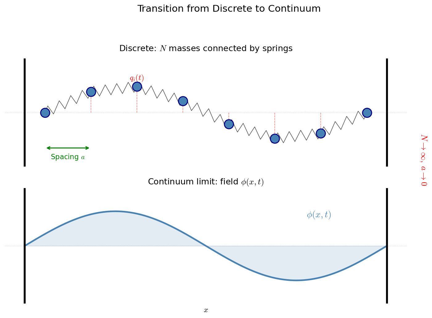
Fig. D.2: A discrete system of \(N\) masses connected by springs (top) and the continuous field \(\phi(x,t)\) obtained in the continuum limit \(N \to \infty\), \(a \to 0\) (bottom). The discrete displacements \(q_i(t)\) transition to the continuous field \(\phi(x,t)\).
🟡 Lina: Taking the continuum limit \(N \to \infty\), \(a \to 0\), the discrete displacements \(q_i(t)\) transition to a continuous field \(\phi(x, t)\). The index \(i\) is replaced by the continuous variable \(x\). See Fig. D.2 "A discrete system of \(N\) masses connected by springs (top) and the continuous field \(\phi(x,t)\) obtained in the continuum limit \(N \to \infty\), \(a \to 0\) (bottom)"—you can see the correspondence between the discrete system (top) and the continuum limit (bottom) visually.
D.9.2 Lagrangian Density
🟡 Lina: In the continuum limit, the Lagrangian takes the form of a spatial integral:
Here \(\mathcal{L}\) is called the Lagrangian density. For example, for string vibrations:
Here \(\mu\) is the linear mass density (mass per unit length) and \(\tau\) is the tension—let's see concretely how these arise from the discrete system's parameters.
🟡 Lina: Let me show the correspondence in the continuum limit. The key point is "rewriting \(\sum_i\) as \(\int dx\)." Since the spacing between adjacent masses is \(a\), the position of the \(i\)-th mass is \(x_i = ia\). As \(a \to 0\) and masses become continuously distributed, \(\sum_i a\) transitions to \(\int dx\) by the method of Riemann sums—the \(\Delta x\) in \(\int_a^b f(x)\,dx = \lim_{N\to\infty}\sum_{i=1}^N f(x_i)\,\Delta x\) that you learned in high school corresponds to \(a\).
🔵 Kai: Ah, \(\sum_i a\) has the same structure as adding up rectangles of width \(a\). But the original equation (D.51) has \(\sum_i\), not \(\sum_i a\), right?
🟡 Lina: Good point. Since the original \(\sum_i\) doesn't contain \(a\), we need to rewrite each term in the form "\(a \times\) (something)." That is, we transform \(\sum_i (\cdots) = \sum_i a \cdot \frac{(\cdots)}{a}\). This way the \(\sum_i a\) part transitions to \(\int dx\), and the \(\frac{(\cdots)}{a}\) part becomes the Lagrangian density \(\mathcal{L}\).
First the kinetic energy term. Rewrite \(\frac{1}{2}m\dot{q}_i^2\) as \(a \cdot \frac{1}{2}\frac{m}{a}\dot{q}_i^2\). With \(\sum_i a \to \int dx\), \(m/a\) becomes "mass per unit length," i.e., the linear density \(\mu\). So we get \(\frac{1}{2}\mu\dot{\phi}^2 = \frac{1}{2}\mu(\partial\phi/\partial t)^2\).
🔵 Kai: I see—you extract one factor of \(a\) to use for the \(\int dx\) conversion, and the rest becomes a density. Same strategy for the potential term?
🟡 Lina: Exactly. Next the potential term. \((q_{i+1} - q_i)/a\) is "the displacement difference between neighbors divided by the spacing," which approaches the spatial derivative \(\partial\phi/\partial x\) as \(a \to 0\). Here too we use the "extract one \(a\)" strategy—the goal is to get the form \(\sum_i a \cdot (\text{something})\) so that with \(\sum_i a \to \int dx\), the "something" becomes the Lagrangian density.
⚪ Mei: So the operation of dividing or multiplying discrete system parameters by \(a\) converts them into "densities."
🟡 Lina: Right. First rewrite the original term \(\frac{1}{2}\kappa(q_{i+1}-q_i)^2\) as \(\frac{1}{2}\kappa a^2 \left(\frac{q_{i+1}-q_i}{a}\right)^2\)—since \((q_{i+1}-q_i)^2 = a^2\left(\frac{q_{i+1}-q_i}{a}\right)^2\). Then decompose \(\kappa a^2 = a \cdot (\kappa a)\). This gives the form \(a \cdot \frac{1}{2}\kappa a \left(\frac{q_{i+1}-q_i}{a}\right)^2\), where one factor of \(a\) is used for the \(\sum_i a \to \int dx\) conversion, and the remaining \(\kappa a\) stays as a physical parameter. Defining the tension as \(\tau = \kappa a\), the integrand becomes \(\frac{1}{2}\tau(\partial\phi/\partial x)^2\).
🔵 Kai: Ah, I see—\(a\) plays two roles. One is used for the "\(\sum_i a \to \int dx\)" conversion, and the other remains inside the physical parameter. But why does \(\kappa a\) become the tension? Do the dimensions work out?
🟡 Lina: Good check. The dimensions of the spring constant \(\kappa\) are [force/length], so \(\kappa a\) has dimensions [force/length]×[length] = [force]—indeed the dimensions of tension. Physically, when springs with constant \(\kappa\) are spaced at intervals \(a\), the force pulling the whole thing (tension) is determined by the product of \(\kappa\) and \(a\).
⚪ Mei: Summarizing: \(\mu = m/a\) is the linear density and \(\tau = \kappa a\) is the tension. The distribution of \(a\) differs between the kinetic and potential terms because \(a\) enters the original expressions differently.
🟡 Lina: Exactly. To summarize, the discrete system's \(\frac{1}{2}m\dot{q}_i^2\) corresponds to \(\frac{1}{2}\mu(\partial\phi/\partial t)^2\), and \(\frac{1}{2}\kappa(q_{i+1}-q_i)^2\) corresponds to \(\frac{1}{2}\tau(\partial\phi/\partial x)^2\).
🔵 Kai: In the discrete system it was "the \(i\)-th mass," and in the continuous system it becomes "the field value at position \(x\)." But when \(a \to 0\), the number of masses goes to infinity, right? It's surprising that the same procedure still works.
🟡 Lina: Good intuition. The reason "it works" is that the canonical quantization recipe depends only on the structure of "finding a pair of canonical variables for each degree of freedom and imposing commutation relations," and doesn't essentially depend on whether the number of degrees of freedom is finite or infinite. I'll show specifically how things translate in D.9.3, but to state the conclusion first: in the discrete system we had \([\hat{q}_i, \hat{p}_j] = i\hbar\,\delta_{ij}\), and in the continuous system we simply replace it with \([\hat{\phi}(x), \hat{\pi}(x')] = i\hbar\,\delta(x-x')\)—formally the same pattern repeated. However, precisely because the number of degrees of freedom becomes infinite, quantum field theory exhibits new phenomena absent in particle quantum mechanics—such as particle creation and annihilation.
🔵 Kai: Hmm... the formalism is the same, yet just by having infinitely many degrees of freedom, completely different phenomena like particle creation emerge. Specifically, where does the story of "particles being born" come in?
🟡 Lina: Sharp question. The key point is that when you Fourier-expand the field, each mode becomes an independent harmonic oscillator—as we saw in Ch. 27. The creation operator \(\hat{a}^\dagger\) of each mode corresponds to the operation of "adding one particle." Because the commutation relation \([\hat{a}, \hat{a}^\dagger] = 1\) creates a ladder that raises and lowers particle number, the particle number can change. It's precisely because the formalism is the same that we can confidently extend it, but new physics emerges from having infinitely many degrees of freedom—that's the fascination of quantum field theory. See Ch. 27 for details.
⚪ Mei: Organizing: the discrete → continuous correspondence is: index \(i\) → coordinate \(x\), displacement \(q_i(t)\) → field \(\phi(x,t)\), sum \(\sum_i\) → integral \(\int dx\), and physical parameters become \(m/a \to \mu\) (linear density), \(\kappa a \to \tau\) (tension).
🟡 Lina: Exactly. So equation (D.51) becomes the form of equation (D.53) in the continuum limit, with the integrand being precisely the Lagrangian density \(\mathcal{L}\) of equation (D.54)—everything emerges naturally from the \(a \to 0\) limit operation. Written explicitly:
This is the continuum limit of the discrete system (D.51).
D.9.3 Canonical Quantization of Fields
🟡 Lina: We apply exactly the same procedure as canonical quantization of the discrete system, now to the field:
Table D.3: Correspondence between canonical quantization of discrete and continuous field systems
| Discrete system | Continuous system (field) |
|---|---|
| Generalized coordinate \(q_i(t)\) | Field \(\phi(x, t)\) |
| Canonical momentum \(p_i = \frac{\partial L}{\partial \dot{q}_i}\) | Canonical momentum density \(\pi(x,t) = \frac{\partial \mathcal{L}}{\partial \dot{\phi}}\) |
| \(\{q_i, p_j\} = \delta_{ij}\) | \(\{\phi(x), \pi(x')\} = \delta(x - x')\) |
| \([\hat{q}_i, \hat{p}_j] = i\hbar\,\delta_{ij}\) | \([\hat{\phi}(x), \hat{\pi}(x')] = i\hbar\,\delta(x - x')\) |
🔵 Kai: The Kronecker delta just becomes a delta function, and the structure is exactly the same.
⚪ Mei: The Kronecker delta \(\delta_{ij}\) is replaced by the Dirac delta function \(\delta(x - x')\)—a natural extension from discrete to continuous.
🟡 Lina: Right. Let me supplement just in case: the Dirac delta function was introduced in Appendix C, but let me confirm its meaning here. \(\delta(x - x')\) is a special function that "is infinite only at \(x = x'\), zero everywhere else, and integrates to 1 over all space." It plays the same role for continuous variables that \(\delta_{ij}\) ("1 when \(i = j\), 0 otherwise") played for discrete ones.
⚪ Mei: The continuous version of the Kronecker delta. The tool for "determining whether it's the same point" is \(\delta_{ij}\) in the discrete case and \(\delta(x-x')\) in the continuous case.
🟡 Lina: Exactly. This "canonical quantization of fields" is precisely the starting point of quantum field theory. Quantizing the electromagnetic field gives rise to photons; quantizing the Dirac field gives rise to electrons and positrons. The answer to "why particles alone are insufficient," which we glimpsed in Ch. 27, lies right here.
🔵 Kai: Quantizing particle mechanics gives quantum mechanics. Quantizing field mechanics gives quantum field theory. The same "canonical quantization" recipe can be used for both.
🟡 Lina: Perfect understanding. The quantum mechanics of the main text is "canonical quantization of finitely many degrees of freedom." Quantum field theory is "canonical quantization of infinitely many degrees of freedom (continuous systems)." The tool is the same; only the object it's applied to differs.
✅ Comprehension Check: State the difference between quantum mechanics and quantum field theory from the perspective of canonical quantization in one sentence.
Answer
Quantum mechanics is the canonical quantization of finitely many degrees of freedom (particle coordinates and momenta), while quantum field theory is the canonical quantization of infinitely many degrees of freedom (continuous fields and their canonical momentum densities). The canonical quantization recipe applied is the same, but the number of degrees of freedom of the target system differs.
✅ Comprehension Check: In the canonical quantization of fields, what corresponds to the Kronecker delta \(\delta_{ij}\) of the discrete system?
Answer
The Dirac delta function \(\delta(x - x')\). As discrete indices \(i, j\) are replaced by continuous coordinates \(x, x'\), the Kronecker delta is also replaced by the delta function.
Preview of Next Chapter
🟡 Lina: In this Appendix, we've surveyed the entire path from the Lagrangian and Hamiltonian formalisms of classical mechanics to canonical quantization into quantum mechanics.
🔵 Kai: Newton's \(F = ma\) → Lagrangian and action → Hamiltonian and phase space → Poisson brackets → canonical quantization → Schrödinger equation. It's all connected. But when we move to quantum field theory, are there new "translation barriers"?
🟡 Lina: Good question. Canonical quantization of fields is the entrance to quantum field theory (QFT). The door to the world previewed in Ch. 27 has now been formally opened. New difficulties—such as handling infinities (renormalization)—certainly exist, but the starting toolkit is the same as what we learned today.
⚪ Mei: If we proceed to quantum field theory, phenomena like particle creation and annihilation, antiparticles, and vacuum fluctuations can be described naturally.
🟡 Lina: Exactly. If you want to study quantum field theory further, the tools from this Appendix—especially the concepts of Lagrangian density and canonical momentum density—will be your starting point. Building on the quantum mechanics of the main text, please venture into the world beyond.
Exercises
📝 Exercises:
- Derive the Euler-Lagrange equations from the Lagrangian in 2D polar coordinates → Problem M-1. Derivation of Euler-Lagrange Equations in 2D Polar Coordinates
- Write the Hamiltonian for a 2D central force \(V(r)\) in polar coordinates and derive Hamilton's equations → Problem B-2. Construction of the Hamiltonian via Legendre Transform
- Compute all Poisson brackets of the angular momentum \(L_z = xp_y - yp_x\) with \(x, y, p_x, p_y\) → Problem B-8. Calculation of Poisson Brackets
- Starting from the classical Lagrangian of a charged particle in an electromagnetic field, find the canonical momenta, derive the Hamiltonian, and perform canonical quantization → Problem A-1. Canonical Quantization of a Charged Particle in an Electromagnetic Field
References
-
Lancaster, T. & Blundell, S. J., Quantum Field Theory for the Gifted Amateur (Oxford University Press, 2014), Ch.2 "Lagrangians" & Ch.6 "A first stab at relativistic quantum mechanics" — Careful introduction to the Lagrangian formalism, functional derivatives, Hamiltonians, and Poisson brackets. Ideal as a bridge to quantum field theory.
-
Sakurai, J. J. & Napolitano, J., Modern Quantum Mechanics, 3rd ed. (Cambridge University Press, 2021), Ch.2 first half — Time evolution operator, Heisenberg's equation of motion, correspondence with classical mechanics (Poisson brackets → commutators).
-
Shimizu, A., Foundations of Quantum Theory — For Gentle Understanding of Its Essence (Saiensu-sha, 2004), Ch.6 — Rigorous and concise formulation of the canonical quantization procedure. Introduction of the Schrödinger representation.
Feedback on this page
Let us know if something was unclear, incorrect, or could be improved.