Chapter 1: The Successes and Limitations of Newtonian Gravity
Story so far:
In the Prologue, we saw that all physical models are hypotheses, and that general relativity is a model covering a wide range of phenomena including GPS, black holes, gravitational waves, and cosmology. Now we begin this long journey, following it step by step with equations.
Goals of this chapter
- Formulate Newton's gravitational model as a "field theory" (universal gravitation → gravitational potential → Poisson equation), confirm its stunning success (the discovery of Neptune), and then clearly identify two limitations—the precession of Mercury's perihelion and the instantaneous propagation of gravity
- Furthermore, understand the criterion for "when the Newtonian model becomes insufficient" using the dimensionless quantity \(GM/(Rc^2)\)
- Finally, introduce another formulation of Newtonian mechanics—the principle of least action—and re-derive \(F = ma\) from the Euler-Lagrange equation
- This framework will serve as the "common language" used throughout all of general relativity
1.1 The Law of Universal Gravitation — Confirming Our Starting Point
🟡 Lina: In the Prologue, we saw Newton's law of universal gravitation and the four properties of gravity (universality, cannot be shielded, long-range force, extremely weak). Today we'll take that equation as our starting point and rewrite it in the language of "field theory." Let's first confirm the equation.
\(G \approx 6.67 \times 10^{-11}\ \mathrm{N \cdot m^2 / kg^2}\) is the gravitational constant. As we saw in the Prologue, taking the ratio of gravitational to electromagnetic force between two protons gives the staggeringly small value \(\sim 10^{-36}\). Yet gravity dominates the universe because it cannot be shielded, is always attractive, and reaches infinitely far.
🔵 Kai: That's the stuff we heard about last time. Are we going beyond that today?
🟡 Lina: Yes. When we rewrite this equation as a "field theory," the limitations of Newton's model become clearly visible at the level of equations.
✅ Comprehension Check: What is the order of magnitude of the gravitational constant \(G\) in SI units?
Answer
\(G \approx 6.67 \times 10^{-11}\ \mathrm{N \cdot m^2/kg^2}\) (order of \(10^{-11}\)).
📝 Exercises:
- Calculating gravitational acceleration at Earth's surface → Problem B-1. Calculating Gravitational Acceleration at Earth's Surface
1.2 The Gravitational Field and Gravitational Potential — Rewriting Newtonian Gravity as a "Field Theory"
🟡 Lina: Newton's universal gravitation was written in the form of action at a distance, where "two objects directly attract each other." We're going to rewrite this in the form of local action mediated by a "field." Let me proceed in three steps.
Step 1: From Action at a Distance to Local Action — Introducing the Gravitational Field
🟡 Lina: Equation (1.1) is written as "two objects exert force on each other directly across a distance"—action at a distance. But to resolve the problem of force being transmitted instantaneously, we need a mechanism by which force propagates through space. This is where we introduce the concept of a field.
🔵 Kai: What's a "field"?
🟡 Lina: It's a state where some physical quantity is assigned to each point in space. Think of a temperature map in a weather forecast. Each location on the map has a temperature value assigned to it, right? That's a "temperature field." Similarly, if a vector representing the strength of gravity is assigned to each point in space, that's a "gravitational field."
🟡 Lina: From here on, vectors will appear in our equations, so let me establish a notation convention. In high school you probably represented vectors with arrows \(\vec{r}\), but in university-level physics and beyond, the standard is to use boldface \(\mathbf{r}\). When equations have many subscripts, arrows become hard to read, so the convention in print is to use boldface.
🔵 Kai: Are \(\mathbf{r}\) and \(r\) different?
🟡 Lina: \(\mathbf{r}\) is the position vector (having both direction and magnitude), while \(r = |\mathbf{r}|\) is its magnitude (a scalar, just a number). Pay attention to whether it's boldface or not to distinguish them.
Now, when a mass \(M\) is at the origin, the force on a mass \(m\) at position \(\mathbf{r}\) is
Here \(\hat{\mathbf{r}}\) (read as "\(\mathbf{r}\) hat") is the unit vector pointing from the origin in the direction of \(\mathbf{r}\)—a vector with magnitude 1. The hat symbol \(\hat{}\) is the convention for "unit vector," and we'll use it throughout. The minus sign indicates that the force points opposite to \(\hat{\mathbf{r}}\) (toward the center = attractive). In high school you may have only dealt with the magnitude \(F = GMm/r^2\), but in university physics, formulating things with vectors is fundamental. The notation "unit vector × scalar quantity" will appear constantly from now on, so get used to it. If we name the quantity in parentheses \(\mathbf{g}\), then
🔵 Kai: In equation (1.4), \(m\) doesn't appear inside \(\mathbf{g}\)... does that mean the field exists even before you place the test mass?
🟡 Lina: Exactly right. Look at equation (1.4). Since we were able to factor out \(m\) in equation (1.2), \(m\) doesn't remain in the definition of \(\mathbf{g}\)—meaning \(\mathbf{g}\) is a quantity that exists at each point in space before the test mass \(m\) is placed there. It's the "field" itself that mass \(M\) creates in space, and the field exists as a property of space regardless of whether any object is present. Looking at Fig. 1.1 "Vector field of the gravitational field created by a central mass", you can see that all arrows point toward the center, and arrows are longer (force is stronger) closer to the center.
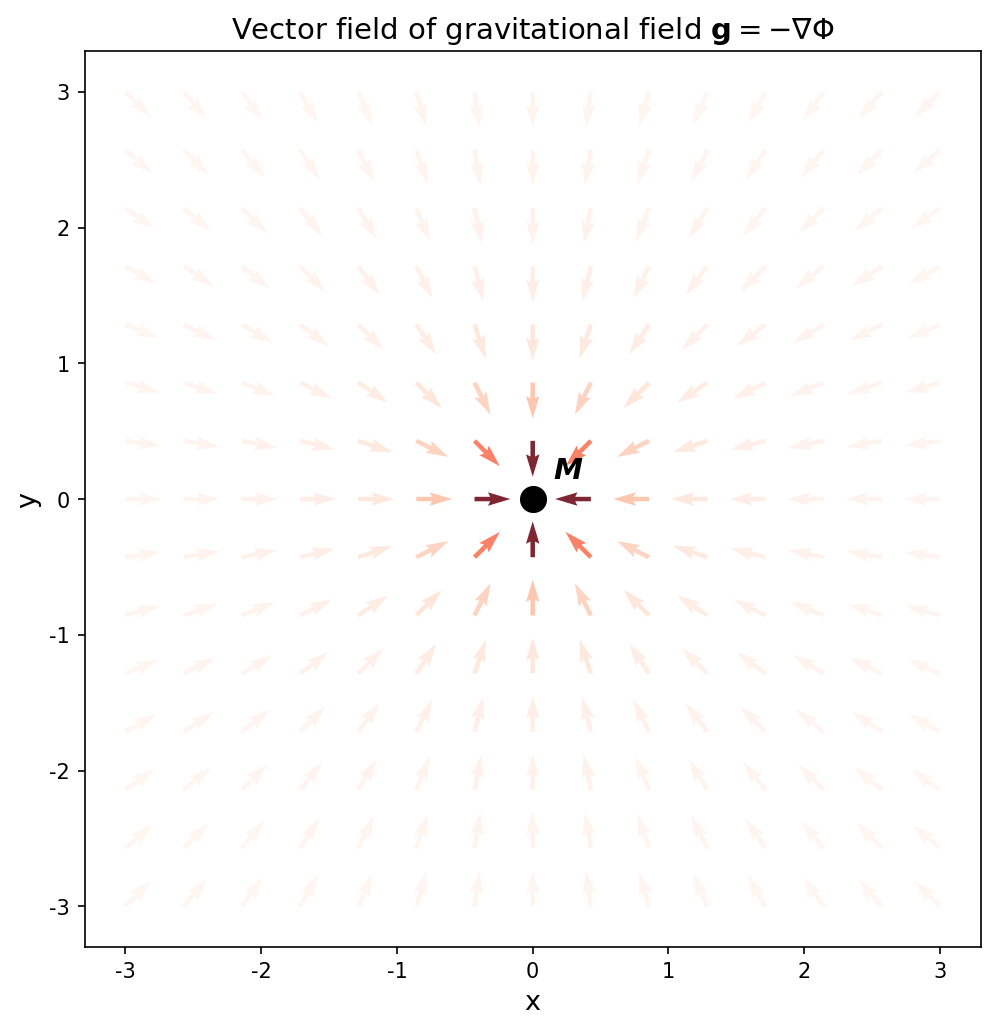
Fig. 1.1: Vector field of the gravitational field created by a central mass. The gravitational field \(\mathbf{g}\) created by a central mass \(M\). All arrows point toward the center, and the force is stronger (darker color) at closer distances.
🟡 Lina: Let me put into words the conceptual shift happening here: "attributing the cause of force to space itself." This is the essence of "field thinking"—local action. We split force transmission into two stages. Stage 1: Mass \(M\) creates a gravitational field \(\mathbf{g}\) in the surrounding space. Stage 2: The gravitational field \(\mathbf{g}\) exerts a force on mass \(m\) at that location. Force is transmitted "through space."
⚪ Mei: So the field is a property of space, not of objects, which means the viewpoint has shifted from "two objects directly attract each other" to "space mediates the force."
🔵 Kai: But even if you say the field "transmits the force," does the transmission take time? Or does it arrive instantaneously?
🟡 Lina: Great question. That's actually a fundamental problem with the Newtonian model—we'll look at it in detail later. First, let's organize the contrast between action at a distance and local action. In action at a distance, two masses exert force on each other directly without any mediator. In local action, mass \(M\) first creates a gravitational field \(\mathbf{g}\) in space, and that field transmits force to mass \(m\)—a two-stage process. Take a look at Fig. 1.2 "Comparison of action at a distance and local action".
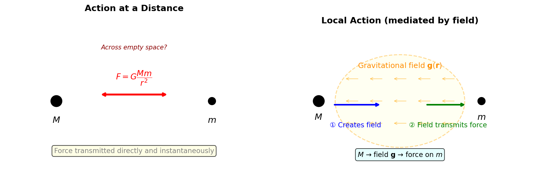
Fig. 1.2: Comparison of action at a distance and local action. Left: In action at a distance, two masses exert force directly on each other without any mediator. Right: In local action, mass \(M\) first creates a gravitational field \(\mathbf{g}\) in space (①), and that field transmits force to mass \(m\) (②).
✅ Comprehension Check: Write the defining equation for the gravitational field \(\mathbf{g}(\mathbf{r})\). What does it mean that this quantity does not depend on mass \(m\)?
Answer
\(\mathbf{g}(\mathbf{r}) = -GM\hat{\mathbf{r}}/r^2\). This quantity does not depend on the test mass \(m\) and is the "field" itself that mass \(M\) creates in space. \(\mathbf{g}\) exists at each point in space before mass \(m\) is placed there.
Step 2: From Vector to Scalar — Introducing the Gravitational Potential
🔵 Kai: But a vector field has 3 directional components at each point, right? Managing that over all of space seems really hard...
🟡 Lina: Good observation. This is where we introduce the gravitational potential \(\Phi(\mathbf{r})\), a scalar field. Since just a single number \(\Phi(\mathbf{r})\) is assigned to each point \(\mathbf{r}\) in space, it's easier to handle than a vector field. What we want to do is "find a scalar function \(\Phi\) whose negative gradient (slope) gives the gravitational field \(\mathbf{g}\)"—that is, find \(\Phi\) such that \(\mathbf{g} = -\nabla\Phi\).
🔵 Kai: What's \(\nabla\)?
🟡 Lina: \(\nabla\) (nabla) is a symbol representing the operation of "taking the gradient." I'll explain the formal definition later in this section, so for now just think of it as "the operation that computes the slope of \(\Phi\)." Don't be intimidated when you see \(\nabla\Phi\)—for the spherically symmetric case, everything can be calculated using just the high school derivative \(d\Phi/dr\), so you can follow all the calculations from here without knowing the formal definition of \(\nabla\). The convention of attaching a minus sign is so that "objects are pulled toward lower potential" is expressed naturally (imagine a ball rolling downhill on a slope). We'll work backward from the already-known \(\mathbf{g}\) to find \(\Phi\). When mass \(M\) is at the origin, spherical symmetry—meaning "it looks the same from any direction"—tells us \(\Phi\) is a function of \(r\) alone. Since there's just a single mass \(M\) sitting at the origin, looking north or east gives the same situation—there's no distinction between the \(x, y, z\) directions. If there's no distinction, the value of \(\Phi\) can't depend on direction either, and must be determined solely by the distance \(r\) from the center. For now, let's find \(\Phi\) using just intuition without waiting for the formal definition of \(\nabla\). If \(\Phi\) is a function of \(r\) alone, then \(\Phi\) only changes in the \(r\) direction. So the "spatial slope of \(\Phi\)" points only in the \(r\) direction (the \(\hat{\mathbf{r}}\) direction), and its magnitude can be calculated with the ordinary derivative \(d\Phi/dr\) from high school. In this special case, "the slope of \(\Phi\)" = "a vector pointing in the \(r\) direction with magnitude \((d\Phi/dr)\)." I'll give the general definition of \(\nabla\) afterward, but for now, a single-variable derivative is all we need. From equation (1.3), the radial component of the gravitational field—the component in the \(\hat{\mathbf{r}}\) direction—is \(g_r = -GM/r^2\) (negative because it points toward the center). On the other hand, writing \(\mathbf{g} = -\nabla\Phi\) in the radial direction only gives \(g_r = -d\Phi/dr\). Setting these equal gives \(-d\Phi/dr = -GM/r^2\), or \(d\Phi/dr = GM/r^2\). We just need to integrate this with respect to \(r\).
⚪ Mei: So the problem of finding the unknown \(\Phi\) reduces to an integration calculation we learned in high school.
🟡 Lina: Right. In Math III you learned \(\int x^n\,dx = x^{n+1}/(n+1)\) (\(n \neq -1\)). The same formula works when the variable is \(r\). Since \(1/r^2 = r^{-2}\), substituting \(n = -2\) gives \(\int r^{-2}\,dr = \frac{r^{-2+1}}{-2+1} = \frac{r^{-1}}{-1} = -\frac{1}{r}\). Using this:
Here \(GM\) is a constant independent of \(r\) so it can be taken outside the integral (the same as \(\int af(x)\,dx = a\int f(x)\,dx\) from high school). \(C\) is the integration constant—since indefinite integrals have an "ambiguity by a constant," we need to fix it with a physical condition. Imposing the boundary condition that \(\Phi \to 0\) at infinity—the convention that "infinitely far away is the reference (zero)"—gives \(-GM/r \to 0\) as \(r \to \infty\), so \(C = 0\) is determined, and we get
🔵 Kai: Oh, it takes the \(-1/r\) form. Zero at infinity, becoming more negative (deeper) as you approach the center.
🟡 Lina: Looking at Fig. 1.3 "3D surface of the gravitational potential", you can see it takes the shape of a "well" that gets deeper as you approach the central mass.
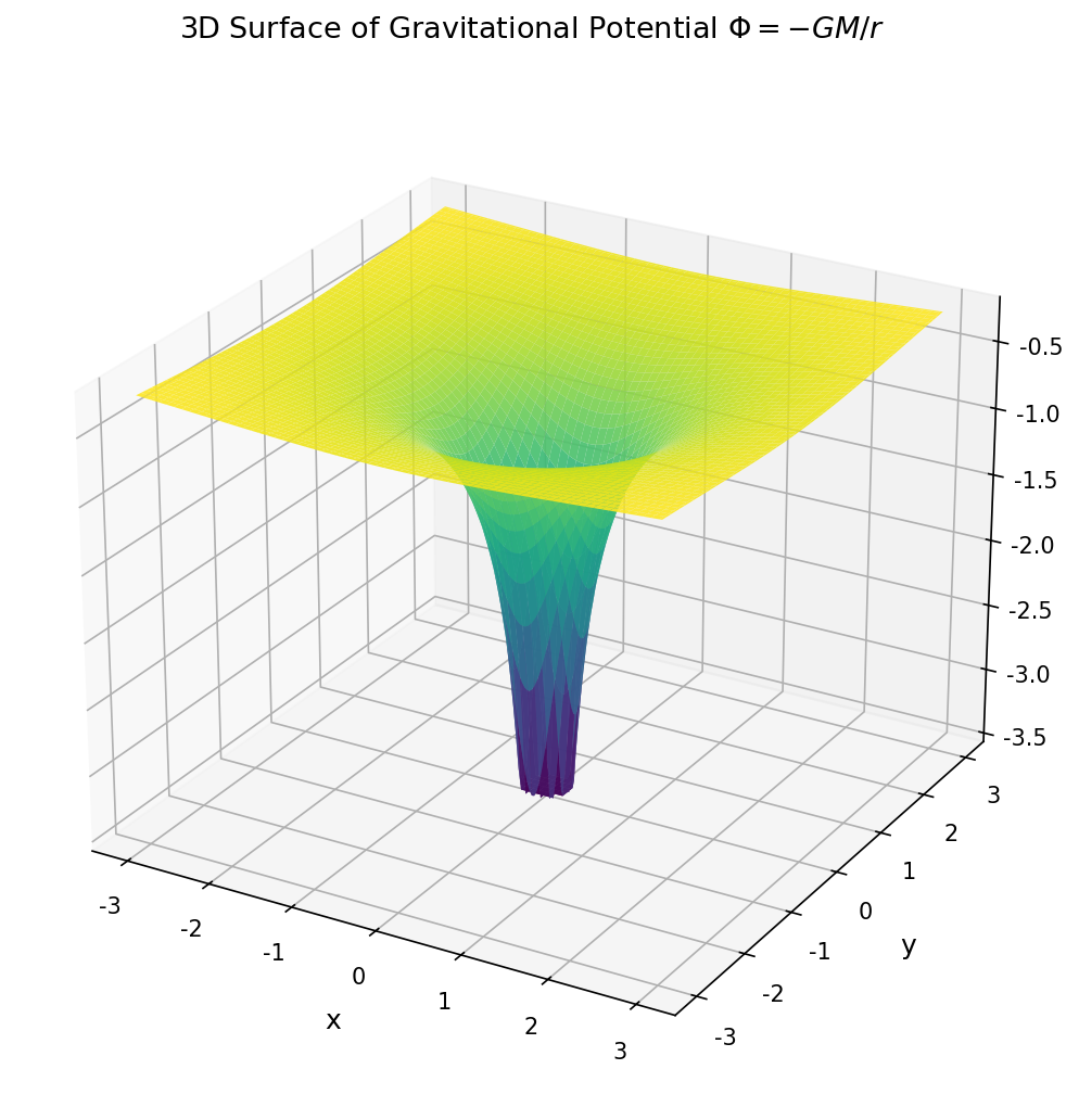
Fig. 1.3: 3D surface of the gravitational potential. The 3D surface of the gravitational potential \(\Phi = -GM/r\). It takes the shape of a "well" that gets deeper as you approach the central mass.
🟡 Lina: Now let's formally define the operation that extracts \(\mathbf{g}\) from \(\Phi\). Earlier we worked backward from \(\mathbf{g}\) to find \(\Phi\), but the natural flow is "given \(\Phi\), compute its slope to obtain \(\mathbf{g}\)." Mathematically this is an operation called the gradient, written with the symbol \(\nabla\) (nabla). In Cartesian coordinates \((x, y, z)\):
That is, the slope in the \(x\) direction, the slope in the \(y\) direction, and the slope in the \(z\) direction, arranged into a single vector. Here \(\partial\) (read "partial"; also called "round" in Japanese physics) is the symbol for partial differentiation. \(\partial\Phi/\partial x\) represents "how much \(\Phi\) changes if you vary only \(x\) slightly while keeping \(y\) and \(z\) fixed." For example, if \(\Phi = x^2 + 3y\), then \(\partial\Phi/\partial x = 2x\) (treating \(y\) as a constant), \(\partial\Phi/\partial y = 3\) (treating \(x\) as a constant), \(\partial\Phi/\partial z = 0\) (since \(\Phi\) doesn't contain \(z\)). It's the same calculation as high school differentiation—you just "differentiate with respect to one variable while treating the others as constants." So \(\nabla\Phi\) is a vector that tells you the direction in which \(\Phi\) increases most rapidly and the magnitude of that slope.
⚪ Mei: So \(\nabla\Phi\) combines "the direction of steepest increase of \(\Phi\) and the magnitude of the slope" into a single vector—like an "arrow pointing in the steepest direction" on a contour map of a mountain.
🟡 Lina: Right. The gravitational field is the negative gradient of the potential:
As I said before, the minus sign is because objects are pulled toward the direction of lower potential—the gradient \(\nabla\Phi\) points "uphill," but gravity pulls "downhill," so the minus sign is needed.
🔵 Kai: So \(\Phi\) is like a "gravitational height," and its slope generates the force.
🟡 Lina: Looking at Fig. 1.4 "Contour lines and gradient of the gravitational potential", you can see that the arrows are perpendicular to the contour lines (lines connecting points of equal \(\Phi\)) and point in the direction of decreasing potential.
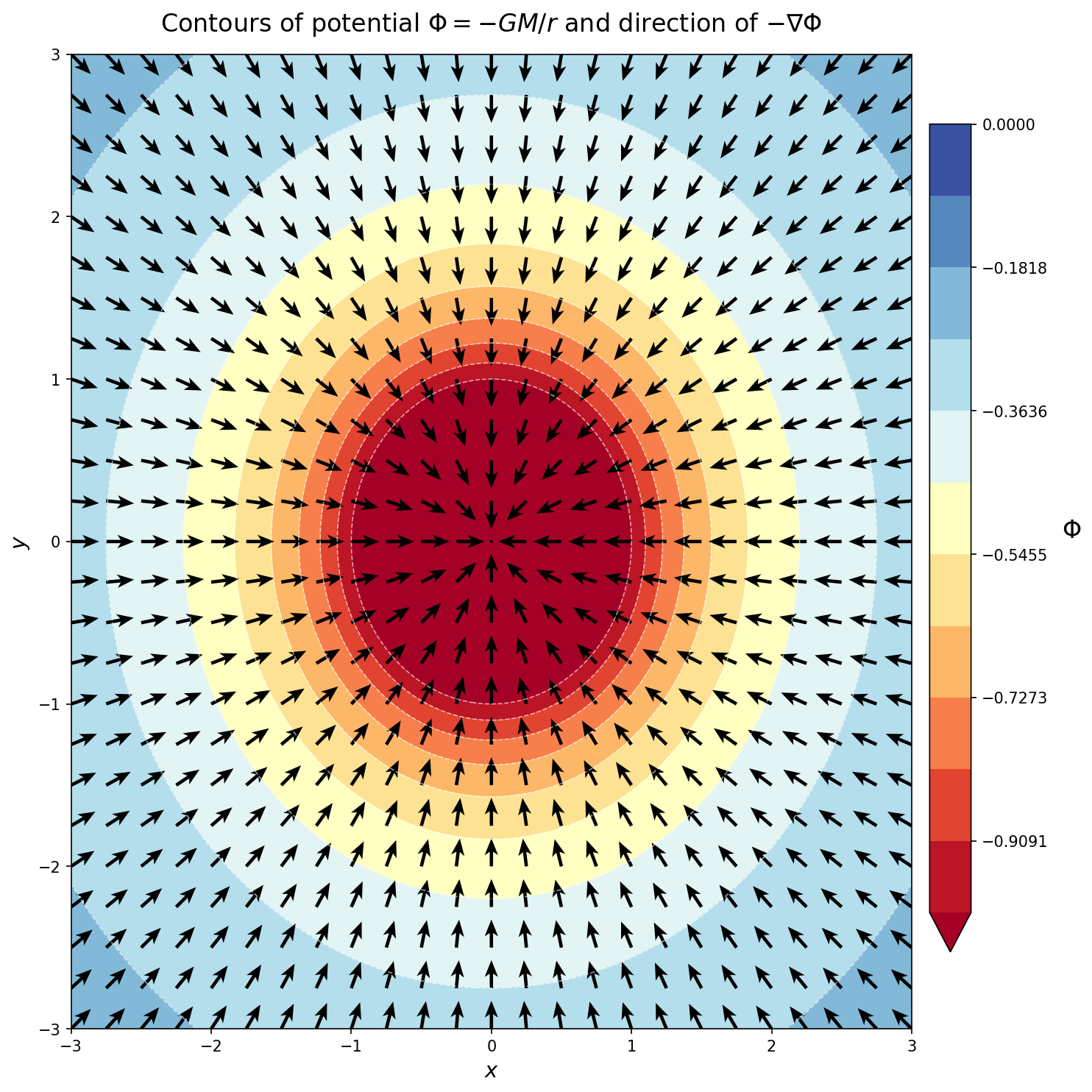
Fig. 1.4: Contour lines and gradient of the gravitational potential. A contour map (colors) of the same potential \(\Phi = -GM/r\) viewed from above, with the direction of the gravitational field \(\mathbf{g} = -\nabla\Phi\) (arrows). The arrows point in the direction of decreasing potential, i.e., toward the mass.
✅ Comprehension Check: Explain the difference between "action at a distance" and "local action" using the concept of the gravitational field.
Answer
Action at a distance: Two objects exert force on each other directly across a distance. Local action: Mass \(M\) first creates a gravitational field \(\mathbf{g}\) in the surrounding space, and that field exerts a force on mass \(m\). Force is transmitted "through space."
✅ Comprehension Check: For the gravitational potential \(\Phi = -GM/r\), \(\Phi \to 0\) as \(r \to \infty\). What does this mean?
Answer
Infinity is chosen as the reference point (zero potential). The potential becomes more negative (deeper) as you approach mass \(M\), representing being bound by gravity.
📝 Exercises:
- Gradient of the gravitational potential → Problem B-2. Differentiation of the \(x\) Component of the Gravitational Potential, Problem B-3. Vector Representation of the Gravitational Field, superposition principle → Problem B-4. Superposition of Two Point Masses, partial derivative practice → Problem B-8. Basic Calculations of Partial Derivatives, Problem B-9. Gradient Vectors and Isotherms, gradient of a 2D potential → Problem B-3. Gradient of a 2D Potential
Step 3: From Point Masses to Distributions — The Poisson Equation
🟡 Lina: So far we've established that "once we know the potential \(\Phi\), the gravitational field is determined by \(\mathbf{g} = -\nabla\Phi\)." The next question is: how is \(\Phi\) determined? Equation (1.5) was the result for the special case of "a point mass \(M\) at the origin." But real stars have size, and mass is spread out through space. So we introduce the "mass density" \(\rho(\mathbf{r})\) (rho)—mass per unit volume.
🔵 Kai: Can you find the potential even when mass is scattered all over space?
🟡 Lina: Yes. Let me pose a question here. "Is there a way to know how much mass is contained in some region, using only information about the potential or gravitational field?"
🔵 Kai: If the gravitational field is strong, there should be a lot of mass inside... but how do you make that quantitative?
🟡 Lina: Good intuition. In fact, the following property can be derived from the inverse-square law. Let me give the intuitive explanation first, then the mathematics. The road to the Poisson equation is a bit long, so let me show you the roadmap first. (1) First understand "flux" and "Gauss's law" → (2) Then use "divergence" and the "divergence theorem" to translate surface properties into pointwise properties → (3) Finally obtain the Poisson equation. Starting with (1). Consider any closed surface surrounding mass \(M\)—like a balloon that completely encloses the mass. At each point on that surface, measure the strength with which the gravitational field "penetrates" the surface, and sum over the entire surface. This is called the flux. Using a water flow analogy, if water comes out of a hose and you catch it with a net, the total amount of water passing through the net corresponds to the flux. For the gravitational field, it's "the total gravitational field strength passing through the surface."
🔵 Kai: If you change the shape of the surface, wouldn't the flux change too...?
🟡 Lina: Remarkably, thanks to the inverse-square law, it doesn't change. Think of it this way. Going back to the water flow example: when water flows uniformly out of a hose, "the amount of water passing through the net" can be calculated as "flow velocity × net area"—the faster the flow and the larger the net, the more water passes through. Gravitational flux works the same way: "field strength × area." For a spherical enclosure, the gravitational field magnitude is uniform at \(GM/r^2\) everywhere on the sphere, and the sphere's surface area is \(4\pi r^2\). Moreover, on the sphere the gravitational field is perpendicular to the surface, so "field strength × area" directly gives the flux, and the \(r^2\) cancels out to give \(4\pi GM\)—independent of the sphere's radius (we'll handle the sign later).
⚪ Mei: The field strength weakens as \(1/r^2\), but the area grows as \(r^2\), so they exactly cancel and become independent of radius—a property unique to the inverse-square law.
🟡 Lina: Exactly. The total doesn't change even if you deform the surface from a sphere. Why? First let me explain the concept of solid angle. In 2D, "angle" represents how wide two lines open, but in 3D we need a quantity representing the "spread of directions." That's the solid angle. For example, if you stretch out your arm and stick up your thumb, the "spread of directions" that your thumbnail occupies in your field of view is the image of solid angle—a large billboard far away and a small business card nearby, if they appear the same size, subtend the same solid angle. It represents how much directional coverage a part of a surface has as seen from the center. The unit is called steradians (sr), and the full sphere (all directions) is \(4\pi\) sr—since the surface area of a sphere of radius \(r\) is \(4\pi r^2\), the total solid angle is \(4\pi r^2 / r^2 = 4\pi\) sr.
Now, what happens when you deform a closed surface? If some part of the surface moves closer to the center, the field is stronger there (increases as \(1/r^2\)). But at the same time, the spread of directions (solid angle) that part covers as seen from the center becomes narrower. The solid angle is determined by "area ÷ \(r^2\)." Just as a 2D angle is "arc length ÷ radius" (the definition of radians)—in 3D it becomes "area ÷ radius squared." A small patch of area \(A\) at distance \(r\) from the center, facing the center (its normal points toward the center), subtends a solid angle \(\Delta\Omega = A/r^2\). The same area subtends less if it's far away and more if it's nearby. If the surface is tilted—if the normal deviates from the radial direction—the "apparent area as seen from the center" decreases (imagine a sign viewed head-on versus at an angle). The solid angle \(\Delta\Omega\) is defined as "apparent area (the component facing the center) ÷ \(r^2\)," so tilting reduces the solid angle contribution even for the same actual area. When the surface moves closer so \(r\) decreases, the area needed to cover the same solid angle decreases proportionally to \(r^2\). Conversely, parts that move farther away have weaker fields but cover more directions. Recall that flux is "perpendicular component of field strength × area." For a small patch: the field strength is \(GM/r^2\), extracting the perpendicular component accounts for tilt, and combined with area gives \(GM \times (\text{apparent area})/r^2 = GM\,\Delta\Omega\), with \(r\) cancelling—each patch's contribution to the flux depends only on the solid angle \(\Delta\Omega\) it subtends, independent of distance \(r\). Over the entire closed surface, all \(4\pi\) of directions are covered, so the total is \(4\pi GM\) (or \(-4\pi GM\) including the sign). It's independent of the surface shape. Look at Fig. 1.5 "Gauss's law: flux through a closed surface".
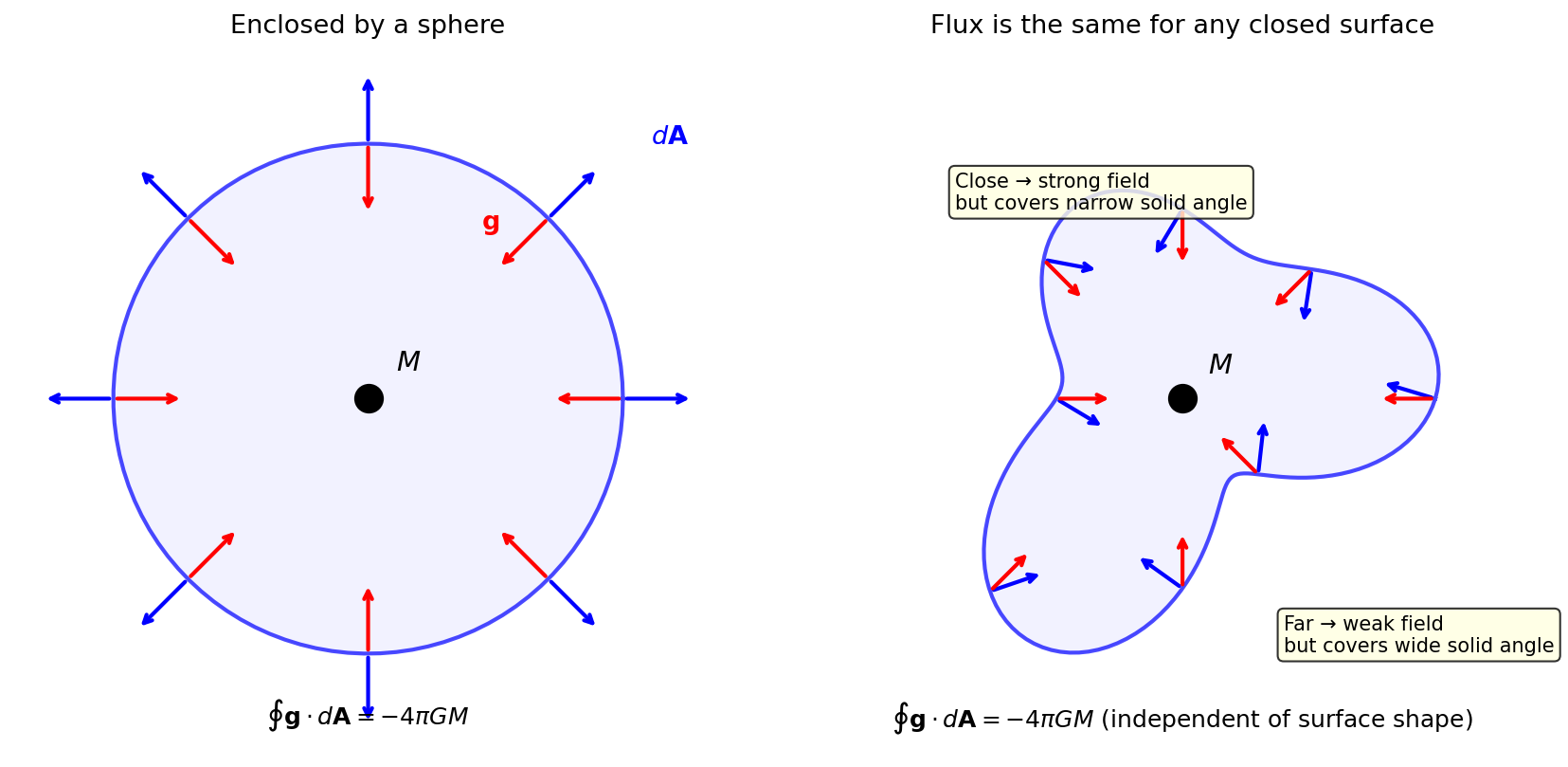
Fig. 1.5: Gauss's law: flux through a closed surface. Left: Enclosed by a sphere. Red arrows are the gravitational field \(\mathbf{g}\) (inward), blue arrows are the area element \(d\mathbf{A}\) (outward). Right: Even for a deformed closed surface, nearby parts have stronger fields but cover less direction (solid angle), while distant parts have weaker fields but cover more direction, so the total flux remains \(-4\pi GM\).
🟡 Lina: Let me write this in equations. There are three things to do—(a) define the tool for measuring "how strongly the gravitational field penetrates the surface" at each point, (b) introduce notation for summing this over the entire surface, (c) actually compute it for a sphere. Starting with (a). Consider a sphere of radius \(r\). Imagine dividing the sphere into small tiles. Each tile has an area and an outward normal direction. In the limit where tiles become infinitesimally small, the vector combining each tile's area and normal direction is written as the area element vector \(d\mathbf{A}\)—its magnitude is the infinitesimal area, and its direction is the outward normal. This is the same idea as making \(\Delta x\) infinitesimally small to get \(dx\) in high school integration. For a sphere, the normals all point radially outward (in the \(\hat{\mathbf{r}}\) direction).
🔵 Kai: So the area element vector combines each tile's "area" and "which direction it faces" into a single vector?
🟡 Lina: Right. Its magnitude is the tile's area, and its direction is the tile's outward normal. Next, at each tile we compute "the component of the gravitational field perpendicular to the surface." This is expressed by the dot product \(\mathbf{g} \cdot d\mathbf{A}\)—the operation that multiplies the "same-direction components" of two vectors. You may have learned \(\vec{a} \cdot \vec{b} = |\vec{a}||\vec{b}|\cos\theta\) in high school—it's the same thing. On the sphere, \(\mathbf{g}\) and \(d\mathbf{A}\) point in opposite directions (the gravitational field is inward, the area element is outward), so \(\cos\theta = \cos 180° = -1\), and the dot product becomes \(-|\mathbf{g}|\,|d\mathbf{A}|\).
🔵 Kai: The gravitational field is coming "into" the surface, but the area element points "outward," so the product is negative.
🟡 Lina: Exactly. A negative dot product means "the field enters the surface"—since we define outward as positive, absorption is represented as negative. So \(\mathbf{g} \cdot d\mathbf{A}\) means "perpendicular component of the gravitational field × infinitesimal area," which in this case is negative.
⚪ Mei: I see, the positive/negative sign distinguishes "source" from "sink."
🟡 Lina: Right. Finally, the symbol \(\oint\) means "sum over all tiles on a closed surface"—if high school's \(\int\) is "summing along a line," then \(\oint\) is "summing over all tiles on a closed surface." Let's compute concretely on a sphere. The total area of all tiles on the sphere sums to the surface area \(4\pi r^2\). At each tile, \(\mathbf{g} \cdot d\mathbf{A} = -|\mathbf{g}| \times (\text{tile area}) = -(GM/r^2) \times (\text{tile area})\). Summing over all tiles:
The \(r^2\) in the numerator and denominator cancel, giving a result independent of the sphere's radius.
🔵 Kai: Wow, \(r\) really cancels! The result is the same no matter how big you make the sphere.
🟡 Lina: This is called Gauss's law (gravitational version). The minus sign on the right is because the gravitational field points inward (toward the center) while the area element \(d\mathbf{A}\) takes outward as positive. Regardless of the shape or size of the surface, the result depends only on the mass inside—a powerful result.
🔵 Kai: Regardless of shape? Whether it's a sphere or a cube?
🟡 Lina: Yes. The next step is to translate Gauss's law from "a total over the whole surface" to "a property at each point." The mathematical tool for this is the divergence theorem.
🟡 Lina: Let me state the claim first—"the total flux through a closed surface = the sum of the source/sink strength at each interior point, integrated over the volume." Intuitively, divide the interior of the closed surface into many small boxes. On shared faces between adjacent boxes, the flux "going out" of one box and "coming in" to the other cancel each other. What remains uncancelled is only the flux through the outermost faces—the original closed surface. So "the sum of all boxes' source strengths" = "the total flux through the outer surface." Imagine the left panel of Fig. 1.6 "Intuitive image of divergence. Left: Source (positive divergence)" as many small boxes lined up side by side. The rigorous proof can be found in Problem M-1. Derivation of Poisson's Equation from Gauss's Law. Let me first explain what "source/sink strength at each point" means, then write the equations.
🔵 Kai: What does "source/sink strength at each point" mean?
🟡 Lina: Think of it this way. Imagine a tiny box around some point. If the net flux leaving through the box's surface is positive, that point is a "source"—like a faucet where the field is being created. Conversely, if flux enters the box, it's a "sink." For gravity, at locations where mass exists, the gravitational field is absorbed from all directions, so the source strength is negative. Look at Fig. 1.6 "Intuitive image of divergence. Left: Source (positive divergence)".
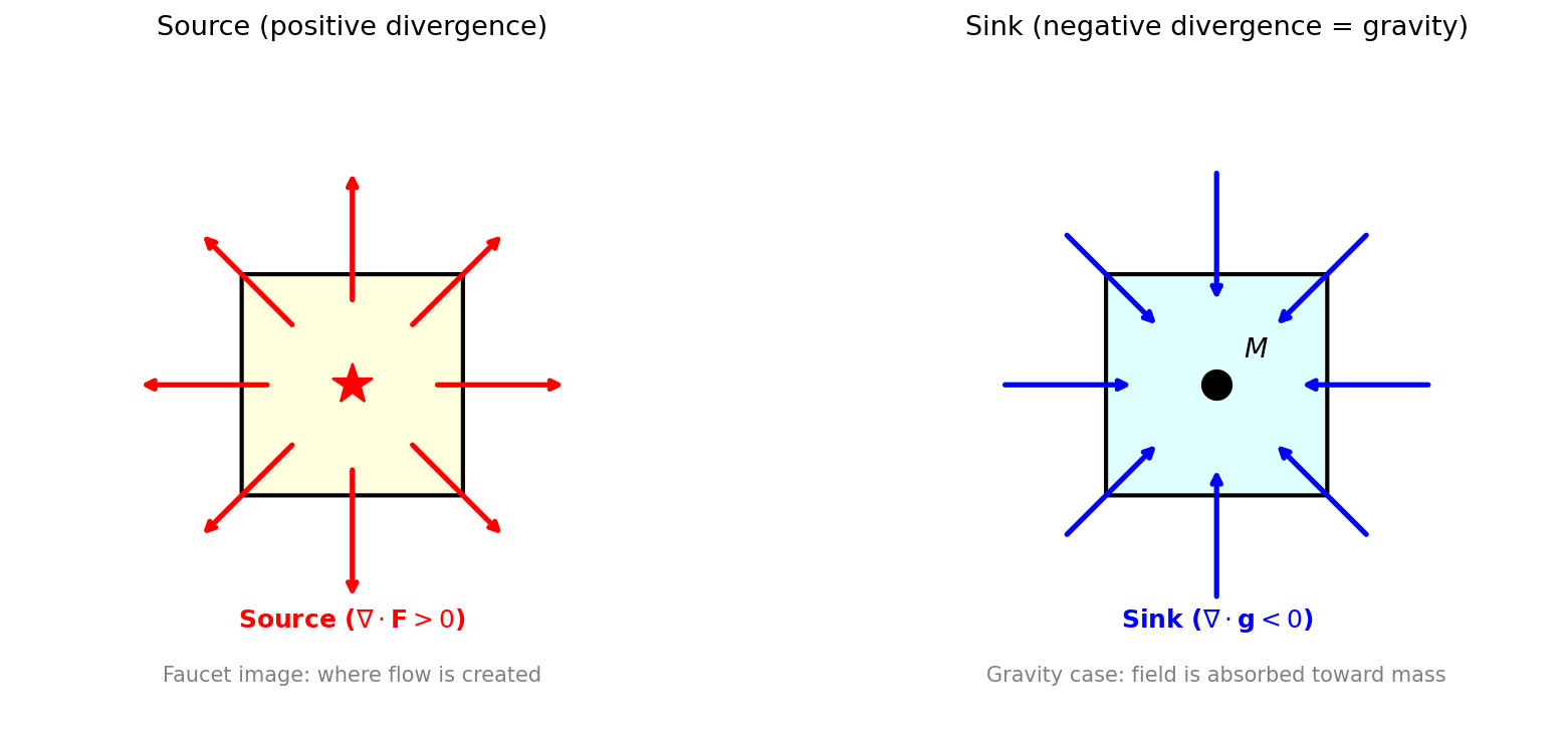
Fig. 1.6: Intuitive image of divergence. Left: Source (positive divergence)—flow exits the box like a faucet. Right: Sink (negative divergence)—in the case of gravity, the field is absorbed toward mass \(M\).
🟡 Lina: The mathematical expression for "the strength of source/sink at each point" is \(\nabla \cdot \mathbf{g}\) (nabla dot g)—a scalar quantity called the divergence of the gravitational field. In Cartesian coordinates:
That is, the sum of how much each component of the gravitational field changes in each direction. While the gradient \(\nabla\Phi\) was an operation creating a vector from a scalar, the divergence \(\nabla \cdot \mathbf{g}\) is an operation creating a scalar from a vector. The divergence theorem says "the total flux through a closed surface = the sum of source/sink strengths at interior points integrated over volume." In equations:
The left side, "total flux through the surface," equals the right side, "sum of source/sink contributions from all interior points."
🔵 Kai: So you can rewrite the total through the surface as "the total of contributions from each point inside."
🟡 Lina: Yes. On the right side of Gauss's law \(-4\pi GM\), \(M\) is the total mass inside the closed surface, so we can write \(M = \int \rho\, dV\) (density integrated over volume). Here \(\int \rho\, dV\) is the operation of "multiplying the density \(\rho\) at each point by the infinitesimal volume \(dV\) and summing over everything"—if high school's \(\int f(x)\,dx\) is "summing along a line," then \(\int \rho\, dV\) is "summing over the entire volume." So the right side is \(-4\pi G \int \rho\, dV\). Applying the divergence theorem to the left side gives \(\int_V (\nabla \cdot \mathbf{g})\, dV = -4\pi G \int_V \rho\, dV\). This equality holds for any region \(V\) we choose—if the integrands were not equal at some point, say \(\nabla \cdot \mathbf{g} > -4\pi G\rho\) at some point, we could choose a very small region \(V\) containing that point, and the left side would exceed the right, breaking the equality. Therefore the integrands must be equal at every point (this argument will be used again in deriving the Euler-Lagrange equation):
⚪ Mei: A "relationship over the whole surface" has been translated into "a relationship at each point"—a very strong conclusion.
🟡 Lina: The minus sign is because the gravitational field is "absorbed" toward mass. Substituting \(\mathbf{g} = -\nabla\Phi\) gives \(\nabla \cdot (-\nabla\Phi) = -4\pi G\rho\), i.e., \(-\nabla^2\Phi = -4\pi G\rho\). Multiplying both sides by \(-1\) to flip the signs gives the Poisson equation:
The proof of the divergence theorem itself can be found in Problem M-1. Derivation of Poisson's Equation from Gauss's Law.
🔵 Kai: What's this \(4\pi\) in the equation? Why does pi appear?
🟡 Lina: The \(4\pi\) comes from Gauss's law. Look at the earlier equation \(\oint \mathbf{g} \cdot d\mathbf{A} = -4\pi GM\). When a point mass \(M\) is enclosed by a sphere of radius \(r\), the sphere's surface area is \(4\pi r^2\). The magnitude of the gravitational field is \(GM/r^2\), and its direction is toward the center (inward). Meanwhile, the area element \(d\mathbf{A}\) takes outward as the positive direction, so \(\mathbf{g}\) and \(d\mathbf{A}\) are opposite—the dot product is negative. The flux is \(-(GM/r^2) \times 4\pi r^2 = -4\pi GM\), matching the right side exactly. So \(4\pi\) is a geometric factor arising from the surface area of a sphere. It appears naturally from the combination of the inverse-square law and the spherical symmetry of 3-dimensional space.
🔵 Kai: What's \(\nabla^2\)?
🟡 Lina: It's an operator called the Laplacian, and in Cartesian coordinates \((x, y, z)\):
It's the sum of the second derivatives of \(\Phi\) in each direction. The gradient \(\nabla\Phi\) from before was a vector (having direction and magnitude), but \(\nabla^2\Phi\) is a scalar (just a number). In high school you learned that \(f''(x) > 0\) means "the graph is concave up." Concave up means the value \(f(x)\) at that point is less than the average of nearby values to the left and right—meaning "it's depressed relative to its surroundings." Conversely, \(f''(x) < 0\) means concave down, and the point is higher than its surroundings. \(\nabla^2\Phi\) is the 3-dimensional generalization of "how much the value deviates from the surrounding average." More precisely, \(\nabla^2\Phi(P)\) is proportional to "average of surrounding values − the central value \(\Phi(P)\)"; if positive, the center is depressed (lower) relative to surroundings. Look at Fig. 1.7 "Intuitive meaning of the Laplacian".
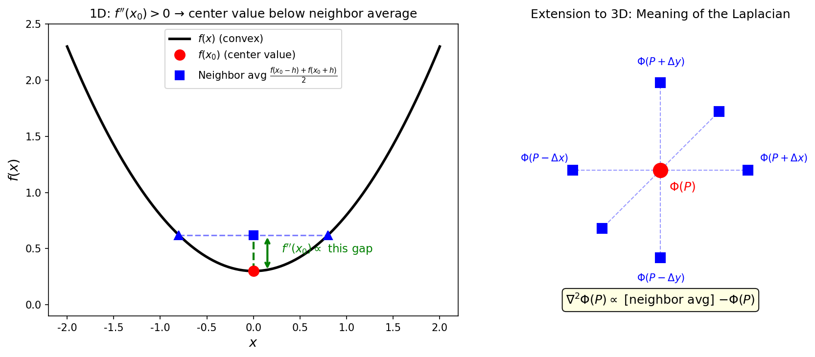
Fig. 1.7: Intuitive meaning of the Laplacian. Left: The 1D case. If \(f''(x_0) > 0\) (concave up), the central value \(f(x_0)\) is lower than the average of its neighbors. Right: Extension to 3D. The Laplacian \(\nabla^2\Phi(P)\) is proportional to "average of surrounding points − central value \(\Phi(P)\)" (positive means the center is depressed).
🟡 Lina: Let me summarize the three differential operations that have appeared so far in a table.
Table 1.1: Three differential operations in vector calculus
| Operation | Symbol | Input → Output | Physical meaning |
|---|---|---|---|
| Gradient | \(\nabla\Phi\) | Scalar → Vector | Direction of steepest increase and its slope |
| Divergence | \(\nabla\cdot\mathbf{g}\) | Vector → Scalar | Source/sink strength at each point |
| Laplacian | \(\nabla^2\Phi\) | Scalar → Scalar | Deviation from the surrounding average |
⚪ Mei: The input and output types are all different. The gradient creates a vector from a scalar, and the divergence returns a scalar from a vector. So if you apply these two in succession, you get "scalar → vector → scalar," returning to the original type... is that the Laplacian in the third row?
🟡 Lina: Yes. And what I want you to notice is that applying rows 1 and 2 in succession gives scalar → vector → scalar. In fact \(\nabla^2\Phi = \nabla \cdot (\nabla\Phi)\)—the Laplacian is the two-stage composition of "taking the gradient, then taking the divergence." Since it's a two-stage composition of scalar → vector → scalar, row 3 is the combination of rows 1 and 2. When we earlier substituted \(\mathbf{g} = -\nabla\Phi\) into \(\nabla \cdot \mathbf{g} = -4\pi G\rho\) and got \(\nabla^2\Phi\), it was precisely this structure.
🔵 Kai: I see—the three operations looked separate, but the Laplacian is actually the combination of the first two.
🟡 Lina: So equation (1.7) says: "where matter exists (\(\rho \neq 0\)), we have \(\nabla^2\Phi > 0\)—using the earlier intuition, the potential value is lower than the surrounding average (depressed). The more matter, the deeper the depression." This is consistent with the image in Fig. 1.3 "3D surface of the gravitational potential" where the potential forms a deep well at the location of mass.
⚪ Mei: The left side is the curvature of the potential, and the right side is the amount of matter. So the relationship "matter is the source of the gravitational field" is condensed into this single equation.
🟡 Lina: Exactly. Since equation (1.7) is a differential equation, if you plug in the mass distribution \(\rho(\mathbf{r})\) on the right side and solve this equation, you get the potential \(\Phi(\mathbf{r})\), and from there \(\mathbf{g} = -\nabla\Phi\) gives the gravitational field.
Let me introduce a useful tool here. How do you represent "mass concentrated at a single point" using density \(\rho(\mathbf{r})\)? It's zero everywhere except the origin, infinite at the origin, yet integrates over all space to give mass \(M\)—such an "ultimately peaked" function is called the Dirac delta function \(\delta^3(\mathbf{r})\). The superscript 3 means "3-dimensional version"—peaked in all three \(x, y, z\) directions.
🔵 Kai: Zero everywhere except the origin, and infinite at the origin... does such a function exist?
🟡 Lina: Look at Fig. 1.8 "Gaussian limit of the Dirac delta function". It doesn't exist as an ordinary function, but it can be defined mathematically as "an infinitely sharp peak whose integral equals 1." The definition is given by two properties:
- For \(\mathbf{r} \neq 0\): \(\delta^3(\mathbf{r}) = 0\)
- Integrated over all space: \(\int \delta^3(\mathbf{r})\, d^3r = 1\)
In other words, "zero everywhere except the origin, but sums to exactly 1 over all space"—a limiting object.
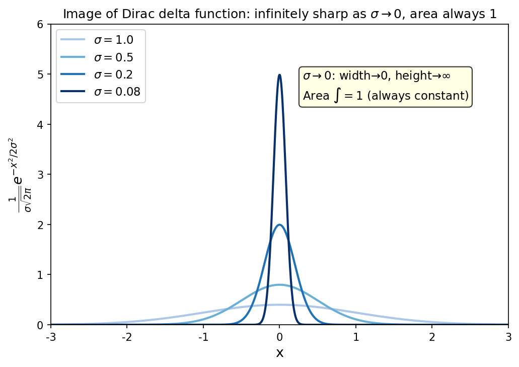
Fig. 1.8: Gaussian limit of the Dirac delta function. Image of the Dirac delta function. As the width \(\sigma\) of a Gaussian function decreases, its height approaches infinity and its width approaches zero, but the area (integral) always remains 1. The \(\sigma \to 0\) limit is the delta function.
🟡 Lina: The mass density of a point mass can be written as \(\rho(\mathbf{r}) = M\,\delta^3(\mathbf{r})\). Since \(\rho = 0\) everywhere except the origin (\(r \neq 0\)), in regions away from the origin the Poisson equation becomes \(\nabla^2\Phi = 0\) (this is called the Laplace equation).
⚪ Mei: Where there is no mass, the Laplacian of the potential is zero—meaning "the surrounding average equals the central value."
🟡 Lina: As in Step 2, spherical symmetry means \(\Phi\) is a function of \(r\) alone. Under this condition, solving \(\nabla^2\Phi = 0\) gives solutions only of the form \(\Phi = A/r + B\). Let me explain briefly why. The Cartesian Laplacian \(\frac{\partial^2\Phi}{\partial x^2} + \frac{\partial^2\Phi}{\partial y^2} + \frac{\partial^2\Phi}{\partial z^2}\) can be rewritten in spherical coordinates \((r, \theta, \phi)\). Spherical coordinates specify a point in space using three quantities: "distance from center \(r\)," "angle from north pole \(\theta\) (complement of latitude)," and "east-west angle \(\phi\) (longitude)"—the same idea as specifying a location on Earth by latitude, longitude, and altitude. It's a more natural coordinate system for spherically symmetric problems than Cartesian coordinates. When \(\Phi\) is a function of \(r\) only, variations with \(\theta\) or \(\phi\) are zero, so only the \(r\)-direction contribution remains in the Laplacian, giving \(\nabla^2\Phi = \frac{1}{r^2}\frac{d}{dr}\left(r^2 \frac{d\Phi}{dr}\right)\).
🔵 Kai: Wait, it's not simply \(d^2\Phi/dr^2\)? Why does \(r^2\) get involved?
🟡 Lina: Good question. Recall that the Laplacian is "deviation from the surrounding average." In 3D, "the surroundings" is a sphere, and its area grows proportionally to \(r^2\). So at larger \(r\), "the surroundings" is wider—the \(r^2\) factor is needed to properly account for this spreading. More concretely, \(\frac{d\Phi}{dr}\) is the "slope in the \(r\) direction," and the radial component of the gravitational field is \(g_r = -d\Phi/dr\). To compute divergence (source/sink strength), we need to look at the "rate of change of flux through spheres." On a sphere of radius \(r\), the radial component of \(\nabla\Phi\) is uniformly \(d\Phi/dr\), so multiplying by the sphere's area \(4\pi r^2\) gives the "total amount of \(\nabla\Phi\) passing through the sphere" as \(4\pi r^2 \frac{d\Phi}{dr}\). Because of spherical symmetry, this is uniform in all directions, and \(4\pi\) remains as a constant throughout. Taking the rate of change in the \(r\) direction gives \(\frac{d}{dr}\left(4\pi r^2 \frac{d\Phi}{dr}\right) = 4\pi \frac{d}{dr}\left(r^2 \frac{d\Phi}{dr}\right)\). Dividing by the shell volume \(4\pi r^2\,dr\) to get "per unit volume," the \(4\pi\) cancels and we get \(\frac{1}{r^2}\frac{d}{dr}\left(r^2 \frac{d\Phi}{dr}\right)\). The detailed coordinate transformation calculation can be checked in Problem B-5. Calculating \(\nabla^2(r^n)\). Setting this equal to zero gives \(\frac{1}{r^2}\frac{d}{dr}\left(r^2 \frac{d\Phi}{dr}\right) = 0\). Since \(1/r^2 \neq 0\), we have \(\frac{d}{dr}\left(r^2 \frac{d\Phi}{dr}\right) = 0\). A quantity whose derivative is zero is a constant (the same as "if \(f'(x) = 0\) then \(f(x) = \text{constant}\)" from high school). So \(r^2 \frac{d\Phi}{dr} = \text{constant}\), i.e., \(\frac{d\Phi}{dr} \propto 1/r^2\). This is the same form as \(d\Phi/dr = GM/r^2\) obtained from the inverse-square law in Step 2. Integrating gives \(\Phi = A/r + B\).
🔵 Kai: I see—solving the Poisson equation in spherical coordinates produces the inverse-square law.
🟡 Lina: The condition \(\Phi \to 0\) at infinity (\(B = 0\)) and the strength condition at the origin give \(A = -GM\), reproducing equation (1.5): \(\Phi = -GM/r\) (the rigorous derivation can be checked in Problem B-6. Laplace Equation Outside a Point Mass). Computing the force from there:
The inverse-square law of gravitation is properly reproduced.
🔵 Kai: Oh, for the point mass case we get the same result as equation (1.1). But since equation (1.7) works even for distributed mass, it's an extension of (1.1)?
🟡 Lina: Exactly. And—this becomes important later—even after rewriting in field language, the Poisson equation contains no time \(t\) whatsoever. This structural problem will be examined in detail in the latter half of this chapter.
✅ Comprehension Check: Write the equation relating the gravitational potential \(\Phi\) and the gravitational field \(\mathbf{g}\).
Answer
\(\mathbf{g} = -\nabla\Phi\). The gravitational field is the negative gradient of the potential. Objects are pulled toward the direction of lower potential.
✅ Comprehension Check: What does the left side \(\nabla^2 \Phi\) of the Poisson equation \(\nabla^2 \Phi = 4\pi G\rho\) physically represent?
Answer
The spatial "curvature" of the potential \(\Phi\) (the sum of second partial derivatives in each direction). Where matter exists (\(\rho \neq 0\)), the potential develops curvature.
✅ Comprehension Check: In the gravitational Gauss's law \(\oint \mathbf{g} \cdot d\mathbf{A} = -4\pi GM\), why doesn't the right side change when you change the shape of the closed surface?
Answer
Because the inverse-square law \(|\mathbf{g}| \propto 1/r^2\) and the sphere's surface area \(4\pi r^2\) cancel each other, so the total gravitational flux through the surface depends only on the mass contained inside, not on the surface shape.
✅ Comprehension Check: State the two properties of the Dirac delta function \(\delta^3(\mathbf{r})\).
Answer
(1) For \(\mathbf{r} \neq 0\): \(\delta^3(\mathbf{r}) = 0\). (2) Integrated over all space: \(\int \delta^3(\mathbf{r})\, d^3r = 1\). Used to express the mass density of a point mass as \(\rho(\mathbf{r}) = M\,\delta^3(\mathbf{r})\).
📝 Exercises:
- Laplacian calculations → Problem B-5. Calculating \(\nabla^2(r^n)\), Problem B-6. Laplace Equation Outside a Point Mass, uniform density sphere → Problem B-7. Potential Constant Inside a Uniform Density Sphere, deriving the Poisson equation from Gauss's law → Problem M-1. Derivation of Poisson's Equation from Gauss's Law, potential of a uniform density sphere → Problem M-2. Complete Potential Solution for a Uniform Density Sphere
1.3 Success Story: The Discovery of Neptune
🟡 Lina: Before moving on to limitations, let's confirm just how powerful Newton's model was. Let me introduce the most dramatic example. The discovery of Neptune.
🔵 Kai: Wasn't Neptune found with a telescope?
🟡 Lina: It was "confirmed" with a telescope. But it was first found on paper with pen. After Uranus was discovered in 1781, astronomers used Newton's model to calculate its orbit. However, the observed position of Uranus deviated slightly from the predicted position.
🔵 Kai: If there's a discrepancy, what do you think? Is the model wrong, or is something being overlooked...?
🟡 Lina: Good question. There are two possibilities: "Newton's model is wrong," or "an undiscovered celestial body is pulling on Uranus." In 1846, France's Le Verrier and England's Adams independently calculated that "if an unknown planet exists at this position, it can explain the deviation in Uranus's orbit." Le Verrier sent a letter to Galle at the Berlin Observatory, asking "point your telescope in this direction."
🔵 Kai: And then?
🟡 Lina: The very night Galle pointed the telescope, a new planet was found within just 1° of the position Le Verrier had predicted. That was Neptune.
🔵 Kai: Amazing! They found a planet just by calculation!
🟡 Lina: This is a real example of "the power of equations" that we discussed in the Prologue. Newton's model gave a quantitative prediction, and that prediction was confirmed by observation. A falsifiable hypothesis withstood verification. The finest success story demonstrating the power of Newton's model.
✅ Comprehension Check: What hypothesis did Le Verrier propose regarding the deviation in Uranus's orbit?
Answer
Rather than "Newton's model is wrong," he hypothesized that "an undiscovered unknown planet is pulling on Uranus" and calculated the predicted position of that planet. Neptune was actually discovered at that position.
✅ Comprehension Check: Why is the discovery of Neptune considered a "success story" for the Newtonian model?
Answer
Because the position of an unknown planet was calculated from Uranus's orbital deviation using Newton's model, and Neptune was actually found within just 1° of that predicted position. A quantitative prediction from equations was confirmed by observation.
1.4 Limitation ①: The Precession of Mercury's Perihelion
🟡 Lina: However, the same Le Verrier also discovered a phenomenon that Newton's model could not explain. The precession of Mercury's perihelion.
🔵 Kai: What's perihelion precession?
🟡 Lina: Planets orbit the Sun in elliptical paths. An ellipse has a point closest to the Sun, called the perihelion. If it were just the Sun and one planet, Newton's model predicts the elliptical orbit repeats the same shape forever. But in reality, gravitational influences from other planets cause the orientation of the ellipse—the position of the perihelion—to slowly rotate. This is perihelion precession.
🔵 Kai: Can't the contribution from other planets pulling on it be calculated with Newton's model?
🟡 Lina: Yes. Le Verrier precisely calculated the influence of all known planets—Venus, Jupiter, Earth, etc.—using Newton's model. However, the calculated and observed values didn't match. The observed perihelion precession of Mercury was larger than Newton's model predicted by about 43 arcseconds per century.
🔵 Kai: How much is 43 arcseconds?
🟡 Lina: One arcsecond is 1/3600 of a degree. So 43 arcseconds is about 0.012 degrees. This much in 100 years. An incredibly small discrepancy.
🔵 Kai: Isn't such a small discrepancy just measurement error?
🟡 Lina: Good question. But the observational precision of 19th-century astronomers was astonishingly high, and this discrepancy far exceeded measurement error. Le Verrier tried the same strategy as with Neptune—"there's an unknown planet"—predicting a planet called Vulcan orbiting inside Mercury's orbit.
🔵 Kai: Was it found like Neptune?
🟡 Lina: No. Despite decades of searching, Vulcan was never found. This is a situation where Newton's model's prediction disagrees with observation—in the language of the Prologue, it's being on the verge of falsification. Newton's model could no longer be called "the best hypothesis not contradicted by experiment."
⚪ Mei: The "unknown planet" hypothesis succeeded with Neptune, but the same strategy failed with Mercury—raising the possibility that there's a problem with the model itself.
🟡 Lina: Look at Fig. 1.9 "Precession of Mercury's perihelion (exaggerated)". It's an exaggerated drawing of how the perihelion of the elliptical orbit rotates slightly with each revolution.
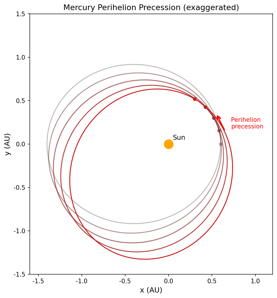
Fig. 1.9: Precession of Mercury's perihelion (exaggerated). The perihelion (point closest to the Sun) of the elliptical orbit rotates slightly with each revolution. Even after accounting for other planets' influences, Newton's model leaves a discrepancy of 43 arcseconds per century.
✅ Comprehension Check: In the problem of Mercury's perihelion precession, Le Verrier tried the same strategy as with Neptune but failed. What was that strategy?
Answer
He assumed an unknown planet Vulcan existed inside Mercury's orbit and predicted it would explain Mercury's orbital discrepancy. However, despite decades of searching, Vulcan was never found, and this strategy failed.
🟡 Lina: This 43-arcsecond discrepancy was explained exactly, with no additional parameters, when Einstein completed general relativity in 1915. Einstein himself said that upon obtaining this calculation result, "for several days I was beside myself with excitement."
✅ Comprehension Check: The discrepancy between Newton's model prediction and observation for Mercury's perihelion precession is approximately how many arcseconds per century?
Answer
Approximately 43 arcseconds. This discrepancy was explained in 1915 by Einstein's general relativity with no additional parameters.
📝 Exercises:
- Scale estimate of Mercury's perihelion precession → Problem M-3. Scale Estimation of Mercury's Perihelion Precession
1.5 Limitation ②: Instantaneous Propagation of Gravity — The Structural Problem of the Poisson Equation
🟡 Lina: The precession of Mercury's perihelion was an empirical problem—a discrepancy with observation. But Newton's model has an even more fundamental problem—one lurking in the structure of the theory itself.
🔵 Kai: A structural problem?
🟡 Lina: Look at the law of universal gravitation (1.1) again.
This equation contains no time \(t\) whatsoever. If the Sun suddenly vanished, \(m_1 = 0\) gives \(F = 0\)—Earth would feel no solar gravity at that instant. Despite being 150 million km away.
🔵 Kai: Light takes about 8 minutes to travel from the Sun to Earth, yet gravitational information arrives in 0 seconds?
🟡 Lina: Yes. This is the problem called instantaneous action at a distance. In fact, Newton himself was dissatisfied with this point. In a letter to a friend, he wrote: "That one body may act upon another at a distance through a vacuum, without the mediation of anything else... is to me so great an absurdity, that I believe no man who has in philosophical matters a competent faculty of thinking, can ever fall into it."
🔵 Kai: Newton himself thought it was "absurd"...
🟡 Lina: And the same structural problem is visible in the Poisson equation (1.7). The left side \(\nabla^2\Phi\) contains only spatial derivatives. There is no time derivative \(\partial^2\Phi/\partial t^2\) anywhere.
🔵 Kai: So the moment \(\rho\) on the right side changes, \(\Phi\) simultaneously changes throughout all of space...?
🟡 Lina: Exactly. The Poisson equation implicitly assumes that changes in the gravitational field propagate at infinite speed. If the Sun suddenly vanished, gravity would disappear at that instant for Earth, 150 million km away.
🔵 Kai: But what's wrong with that?
🟡 Lina: Here, let me borrow just one conclusion from special relativity, which we'll cover in detail in later chapters. According to special relativity, no signal can travel faster than the speed of light \(c \approx 3.0 \times 10^8\ \mathrm{m/s}\). Light takes about 8 minutes to reach Earth from the Sun. The "information" that the Sun has vanished should also take at least 8 minutes.
⚪ Mei: In other words, Newton's gravity implicitly assumes "information propagates instantaneously," which directly contradicts the fundamental principle of special relativity.
🟡 Lina: By contrast, the field equation of electromagnetism (after fixing the freedom remaining in the choice of potential through a mathematical procedure called a "gauge condition") takes this form:
Here \(\varphi\) is the electromagnetic scalar potential (corresponding to gravity's \(\Phi\)), \(\rho_e\) is the charge density (corresponding to gravity's mass density \(\rho\)), and \(\varepsilon_0\) is the permittivity of free space (an electromagnetic constant appearing in Coulomb's law \(F = \frac{1}{4\pi\varepsilon_0}\frac{q_1 q_2}{r^2}\)). The minus sign on the right is due to unit system conventions—don't worry about it now. For now, rather than the details of each symbol, focus on the structure of the equation. This equation has the form of a wave equation. Let me convey just the intuition for why it describes waves propagating at speed \(c\). In one dimension it becomes \(\frac{\partial^2 \varphi}{\partial x^2} = \frac{1}{c^2}\frac{\partial^2 \varphi}{\partial t^2}\). The solution to this equation is \(\varphi(x, t) = f(x - ct)\)—a "wave that moves at speed \(c\) without changing shape."
🔵 Kai: What does it mean that \(f(x - ct)\) is a wave?
🟡 Lina: Think of it this way. Suppose at time \(t = 0\), \(\varphi = f(x)\) has some shape. At time \(t\), \(\varphi = f(x - ct)\). The location where \(f\) takes the same value—say the peak of a hill—satisfies \(x - ct = \text{constant}\), i.e., \(x = ct + \text{constant}\). This moves to the right at speed \(c\). So \(f(x - ct)\) is "a wave that maintains its shape and travels at speed \(c\)."
🔵 Kai: Ah, if you track the position of the peak, it moves to the right by \(c\) every second.
🟡 Lina: Right. Let's verify by substitution. Let \(u = x - ct\). To partially differentiate \(\varphi = f(u)\) with respect to \(x\), use the chain rule from high school: \(\frac{d}{dx}f(g(x)) = f'(g(x)) \cdot g'(x)\). Here \(f'(u)\) means "the ordinary derivative of \(f\) with respect to \(u\)" (since \(f\) is a single-variable function of \(u\), it's a regular derivative, not a partial derivative). Since \(u = x - ct\), we have \(\partial u/\partial x = 1\) (with \(t\) fixed). So \(\frac{\partial \varphi}{\partial x} = f'(u) \cdot 1 = f'(u)\), differentiating again gives \(\frac{\partial^2 \varphi}{\partial x^2} = f''(u)\). On the other hand, differentiating with respect to \(t\): \(\partial u/\partial t = -c\) (with \(x\) fixed), so \(\frac{\partial \varphi}{\partial t} = f'(u) \cdot (-c) = -c\,f'(u)\), differentiating again gives \(\frac{\partial^2 \varphi}{\partial t^2} = (-c)^2 f''(u) = c^2 f''(u)\). Therefore \(\frac{\partial^2\varphi}{\partial x^2} = f''(u)\) and \(\frac{1}{c^2}\frac{\partial^2\varphi}{\partial t^2} = \frac{1}{c^2} \cdot c^2 f''(u) = f''(u)\) are equal, confirming the equation is satisfied.
⚪ Mei: They match beautifully. The \(c^2\) cancels between numerator and denominator, giving \(f''(u) = f''(u)\).
🟡 Lina: The combination of \(\nabla^2\) and \(\frac{1}{c^2}\frac{\partial^2}{\partial t^2}\) is precisely the structure that describes "waves propagating at speed \(c\)." These are electromagnetic waves. In other words, the structure of the equation—whether or not a time derivative is present—determines how changes in the field propagate.
⚪ Mei: So whether or not the field equation contains a second time derivative determines whether "changes propagate instantaneously or as waves at finite speed."
🟡 Lina: Exactly. The structure of the equation governs the physics—the manner of propagation. In source-free regions (\(\rho_e = 0\)), the right side becomes zero, giving a pure wave equation \(\nabla^2\varphi = \frac{1}{c^2}\frac{\partial^2 \varphi}{\partial t^2}\). Placing the gravitational Poisson equation and the electromagnetic wave equation side by side in a table makes the problem immediately apparent.
Table 1.2: Comparison of field equations: Newtonian gravity and electromagnetism
| Newtonian gravity | Electromagnetism | |
|---|---|---|
| Field equation | \(\nabla^2 \Phi = 4\pi G\rho\) | \(\left(\nabla^2 - \frac{1}{c^2}\frac{\partial^2}{\partial t^2}\right)\varphi = -\frac{\rho_e}{\varepsilon_0}\) |
| Time derivative | None | Present (\(\partial^2/\partial t^2\)) |
| Propagation speed | Infinite | Speed of light \(c\) |
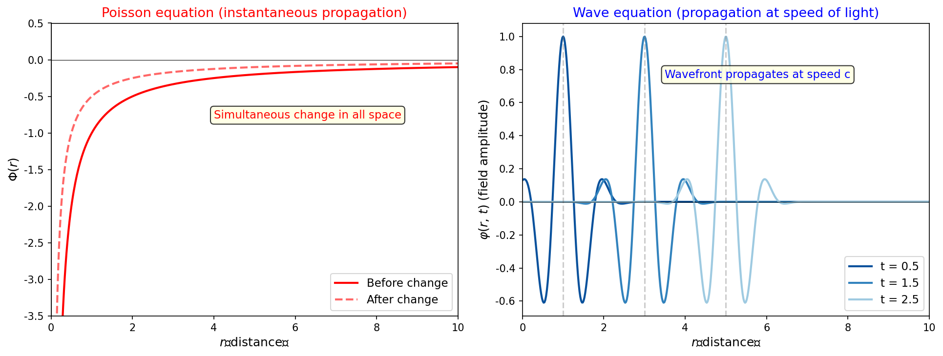
Fig. 1.10: Comparison of the Poisson equation and the wave equation. Left — In the Poisson equation, field changes occur simultaneously throughout all space (instantaneous propagation). Right — In the wave equation, field changes propagate as a wavefront at the speed of light \(c\).
🟡 Lina: The table makes the structural difference immediately clear. Also look at Fig. 1.10 "Comparison of the Poisson equation and the wave equation. Left". On the left, the Poisson equation shows field changes occurring simultaneously throughout all space, while on the right, the wave equation shows them spreading as a wavefront at the speed of light \(c\).
⚪ Mei: Just the presence or absence of a time derivative determines whether the propagation speed is "infinite" or "the speed of light."
🔵 Kai: So does that mean Newtonian gravity is "impossible" in a universe where information travels at light speed? But couldn't you fix it by just adding \(\frac{1}{c^2}\frac{\partial^2}{\partial t^2}\) to Newton's equation...?
🟡 Lina: Good thought. Such attempts were actually made. But simply adding a time derivative term leads to contradictions with other physical requirements. For example, gravity is always attractive (a pulling force), right? But making it a wave equation would allow "repulsive waves" as solutions, conflicting with the observational fact that gravity is always attractive. The correct fix requires something much more fundamental—changing the structure of spacetime itself. That's general relativity. You can check the details in Problem A-1. An Attempt at a Scalar Theory of Gravity.
✅ Comprehension Check: What does the absence of a time derivative \(\partial^2/\partial t^2\) in the Poisson equation mean physically?
Answer
It means changes in the gravitational field propagate at infinite speed (instantaneously). This contradicts special relativity's principle that "no signal can travel faster than the speed of light."
📝 Exercises:
- Contradiction of instantaneous propagation → Problem B-9. Contradiction Between Instantaneous Propagation and Special Relativity, comparison of wave equation and Poisson equation → Problem M-4. Comparison of the Wave Equation and Poisson's Equation, attempt at a scalar gravity theory → Problem A-1. An Attempt at a Scalar Theory of Gravity
🟡 Lina: Therefore, Newton's gravitational model is merely an approximation to a more accurate model. For everyday scales and most aspects of planetary motion in the solar system, Newton's model is astonishingly accurate. But in extreme situations like speeds close to light or very strong gravitational fields, a more accurate model is needed.
1.6 When Does the Newtonian Model Become Insufficient?
🟡 Lina: Finally, let's revisit the criterion introduced in the Prologue. Using a celestial body's mass \(M\) and characteristic radius \(R\)—the surface radius for a star, or the Schwarzschild radius we'll learn about later for a black hole—we compute
a dimensionless quantity.
⚪ Mei: Why does this quantity serve as a criterion?
🟡 Lina: Earlier in this chapter, we learned that the gravitational potential is \(\Phi = -GM/r\) (equation 1.5). Since the potential \(\Phi\) corresponds to "energy per unit mass," the gravitational potential energy of an object of mass \(m\) is \(U = m\Phi\)—a generalization of \(U = mgh\) from high school (near Earth's surface, \(\Phi \approx gh\), so \(U = m\Phi = mgh\)). At the celestial body's surface (\(r = R\)): \(U = m\Phi = -GMm/R\). On the other hand, according to special relativity, an object's rest energy is \(E = mc^2\). Taking the ratio of these two:
The \(m\) cancels, giving a dimensionless quantity determined solely by the celestial body's properties (\(M\) and \(R\)).
🔵 Kai: Ah, it's the ratio of gravitational energy to rest energy. That's why you divide by \(c^2\).
🟡 Lina: Right. When this ratio is small—when gravitational potential energy is much smaller than rest energy—Newton's model is an excellent approximation. But as it approaches 1, the curvature of spacetime that Newton's approximation cannot capture becomes non-negligible. Let me reproduce the table from the Prologue.
Table 1.3: Compactness parameter for representative celestial bodies
| Celestial body | Approximate \(GM/(Rc^2)\) |
|---|---|
| Earth | \(\sim 10^{-9}\) |
| Sun | \(\sim 10^{-6}\) |
| White dwarf | \(\sim 10^{-4}\) |
| Neutron star | \(\sim 0.1\) |
| Black hole | \(\sim 1\) |
⚪ Mei: The smallness of the perihelion precession discrepancy for Mercury (43 arcseconds per century) corresponds to the Sun's \(GM/(Rc^2) \sim 10^{-6}\) being small. The deviation from Newton's model is small but not zero.
🟡 Lina: And as we saw in the Prologue, even Earth's \(10^{-9}\) cannot be ignored in precision technologies like GPS atomic clocks. General relativity is needed not only when \(GM/(Rc^2)\) is large, but also when measurement precision is high enough to be comparable to this value. The values for each celestial body are summarized in Fig. 1.11 "Range of applicability of Newton's model and the relativistic parameter".
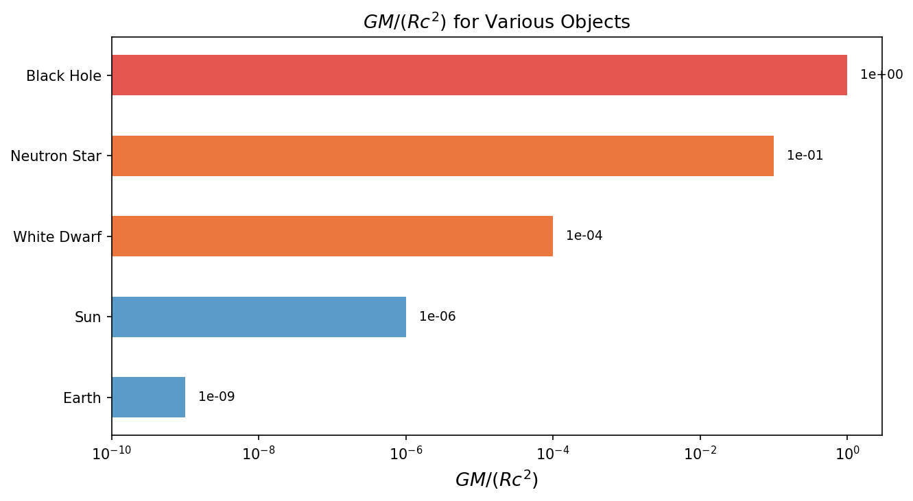
Fig. 1.11: Range of applicability of Newton's model and the relativistic parameter. Values of \(GM/(Rc^2)\) for various celestial bodies. The larger this value, the more pronounced general relativistic effects become.
✅ Comprehension Check: Why might general relativity be needed even for Earth where \(GM/(Rc^2) \sim 10^{-9}\)?
Answer
Because in technologies with extremely high measurement precision, such as GPS atomic clocks, relativistic effects on the order of \(10^{-9}\) cannot be ignored. Even when \(GM/(Rc^2)\) is small, general relativity is needed if measurement precision is high enough to be comparable to that value.
✅ Comprehension Check: What ratio of physical quantities does \(GM/(Rc^2)\) represent?
Answer
The ratio of gravitational potential energy at the celestial body's surface \(|U| = GMm/R\) to rest energy \(E = mc^2\). As this ratio approaches 1, the curvature of spacetime that Newton's approximation cannot capture becomes non-negligible.
📝 Exercises:
- Computing \(GM/(Rc^2)\) → Problem B-10. Estimating Relativistic Effects at the Solar Surface, Problem B-11. Estimating the Relativistic Parameter of a Neutron Star, relationship between escape velocity and \(GM/(Rc^2)\) → Problem B-5. Derivation of the Schwarzschild Radius, Problem B-6. Criterion at the Schwarzschild Radius, shell theorem and tidal forces → Problem A-2. Shell Theorem and Tidal Force
🟡 Lina: Exactly. Newton's model is wonderful as an approximation. But it is only an approximation. The model that goes beyond this approximation is Einstein's general relativity. Before tracing the path to get there, there's one more thing I want to prepare.
1.7 Another Formulation — The Principle of Least Action
🟡 Lina: Let me now change topics and introduce another formulation of Newtonian mechanics.
🔵 Kai: Wait, we were talking about Newton's limitations—why are we introducing a different formulation here?
🟡 Lina: Good question. The reason is that \(F = ma\) won't be usable in the general relativity ahead. In general relativity, gravity is described not as a "force" but as "curvature of spacetime"—an object freely moving through curved spacetime appears to accelerate even though no force acts on it. So the framework of "\(F = ma\)"—"force produces acceleration"—itself becomes unusable. What we'll use instead is the principle of least action that I'm about to introduce. The Ch. 8 geodesic equation, the Ch. 14 Einstein equation, and Appendix C field theory are all derived from this principle. In other words, this becomes the "common language" used in every chapter ahead.
⚪ Mei: So the idea is to get comfortable with the tools while we're still in the familiar territory of Newtonian mechanics.
🟡 Lina: Exactly. Today we'll re-derive \(F = ma\) from the principle of least action. The answer is the same, but the derivation framework is different. Once you master this framework, you'll be able to derive equations of motion using the same procedure even in curved spacetime.
🔵 Kai: The same physics described from a completely different perspective—concretely, how is it different? \(F = ma\) is about "if force is applied, acceleration results"—a cause-and-effect story, right? What other viewpoint is there?
🟡 Lina: Good question. Newton's \(F = ma\) is a causal description—"force determines acceleration"—a chain of cause and effect where "the current force determines the next moment's motion." The principle of least action takes an entirely different approach—"look at the entire path from departure to arrival as a whole, and the path that extremizes a certain quantity is the one realized." It's a "global optimization" perspective, so to speak. Motion is determined not by a chain of causes but by a property of the entire path.
🟡 Lina: Let's look at a concrete example. Toss a ball upward. Newton's method: "at each instant, gravity \(F = -mg\) produces acceleration \(a = -g\)," and you solve the equation of motion by advancing time step by step—"the current force determines the next moment's motion" in a chain of causation.
🔵 Kai: You compute the state at time 1 from time 0, then time 2 from time 1... like dominoes falling one after another.
🟡 Lina: Right. The principle of least action takes a completely different viewpoint. It looks at the entire path from start to finish and determines "which path is naturally selected":
🟡 Lina: "Among all paths a ball could take, the path that extremizes (makes stationary) a quantity called the action is the path the ball actually follows"—this is the principle of least action. Stationary means "the first-order variation is zero"—just as in high school where a point with \(f'(x) = 0\) (a stationary point) could be a maximum or minimum, a path with \(\delta S = 0\) doesn't necessarily minimize the action; it could be a maximum or saddle point. But historically it's called the "principle of least action."
🟡 Lina: Look at Fig. 1.12 "Principle of least action: path selection". The gray lines are examples of "possible paths," and the thick red line is the path nature actually "selects."
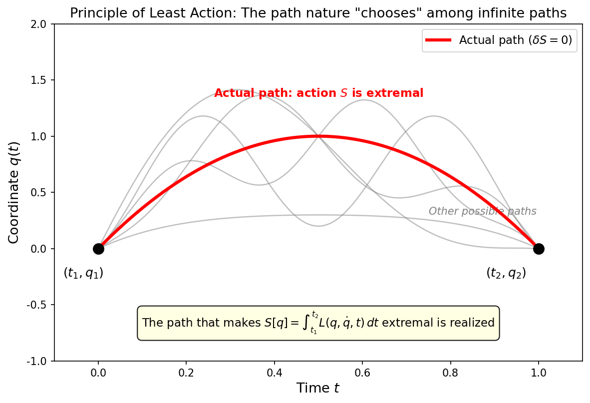
Fig. 1.12: Principle of least action: path selection. Among the countless paths (gray) connecting the start point \((t_1, q_1)\) and end point \((t_2, q_2)\), the path (red) that extremizes the action \(S = \int L\,dt\) is the one physically realized.
🔵 Kai: Action?
Definition of Action and the Lagrangian
🟡 Lina: The action \(S\) is the difference \(L = T - V\) between kinetic energy \(T\) and potential energy \(V\), integrated over time from departure time \(t_1\) to arrival time \(t_2\):
\(L = T - V\) is called the Lagrangian. Here \(T\) is kinetic energy (a function of velocity), \(V\) is potential energy (a function of position)—the same as \(V = mgh\) or \(V = \frac{1}{2}kx^2\) from high school. The dot notation like \(\dot{x}\) represents a time derivative shorthand: \(\dot{x} = dx/dt\) (velocity), \(\ddot{x} = d^2x/dt^2\) (acceleration). For example, the kinetic energy of a particle of mass \(m\) can be written as \(T = \frac{1}{2}mv^2 = \frac{1}{2}m\dot{x}^2\). This notation is used constantly in physics, so remember it.
🔵 Kai: The "difference" of energies, not the "sum"? Why the difference?
🟡 Lina: The principle of least action itself is an axiom, so there's no deep reason for "why \(T - V\)." Newton's \(F = ma\) also can't explain "why this form." Both are justified in the sense that "starting from this principle produces results that agree with experiment." What would happen if we used \(T + V\)? In the upcoming "Recovery of Newton's Equation of Motion" we'll confirm that \(L = T - V\) gives \(m\ddot{x} = -dV/dx\), but if we set \(L = T + V = \frac{1}{2}m\dot{x}^2 + V(x)\), then \(\partial L/\partial x = +dV/dx\), and the Euler-Lagrange equation gives \(m\ddot{x} = +dV/dx\). This predicts "accelerating toward higher potential"—a ball rolling uphill. Only \(T - V\) agrees with experiment.
⚪ Mei: So \(L = T - V\) is "an axiom that produces results agreeing with experiment," and we don't ask "why." Same structure as when the Prologue said "the starting points of a model are not objects of explanation."
Derivation of the Euler-Lagrange Equation
🟡 Lina: Let's derive the equation of motion from the principle of least action. This is the core of the calculus of variations.
What is the calculus of variations: A mathematical method for finding "which path extremizes the action \(S\) among all possible paths?" Ordinary differentiation finds extrema of functions, but the calculus of variations finds extrema of paths (functions themselves).
🟡 Lina: Before doing the actual calculation, let me organize the coordinate notation. From here I'll use the term generalized coordinates.
🔵 Kai: "Generalized coordinates"? Are they different from regular \(x, y, z\)?
🟡 Lina: Good question. Generalized coordinates are the variables chosen to describe the state of a system. They're not limited to Cartesian coordinates \(x, y, z\)—you can freely choose them to suit the problem. For a pendulum, a single angle \(\theta\) determines the state; for a double pendulum, \(\theta_1, \theta_2\). The idea is "you may choose whatever variables you like, as many as the system's degrees of freedom."
⚪ Mei: So \(x\) and \(y\) are special cases of generalized coordinates, and generalized coordinates are about choosing the most natural variables to match the problem's symmetry and constraints.
🟡 Lina: Right. By convention, we use the symbol \(q\). If there are \(n\) degrees of freedom, we write \(q_1, q_2, \ldots, q_n\). For simplicity, I'll proceed with a single degree of freedom \(q(t)\).
✅ Comprehension Check: What are generalized coordinates? How do they differ from Cartesian coordinates \((x, y, z)\)?
Answer
Generalized coordinates are variables freely chosen to describe the state of a system, suited to the problem. Cartesian coordinates are a special case of generalized coordinates; for a pendulum one uses angle \(\theta\), for a double pendulum \(\theta_1, \theta_2\)—choosing variables that match the system's degrees of freedom and symmetry.
🔵 Kai: But we've been writing \(L = T - V\) until now. What changed with \(L(q, \dot{q}, t)\)?
🟡 Lina: The content is the same. For a pendulum, \(T = \frac{1}{2}m l^2 \dot{\theta}^2\), \(V = -mgl\cos\theta\), so writing out \(L = T - V\) gives a function of \(\theta\) and \(\dot{\theta}\). That is, \(L(q, \dot{q}, t)\) is the notation expressing the content of \(T - V\) in terms of generalized coordinate \(q\) and its time derivative \(\dot{q}\). It emphasizes that "the specific form of \(T - V\) differs for each problem, but in every case it can be written in terms of \(q\), \(\dot{q}\) (and sometimes time \(t\))."
🟡 Lina: Given a Lagrangian \(L(q, \dot{q}, t)\) using generalized coordinate \(q(t)\), where \(\dot{q} = dq/dt\) is velocity, the action is:
The square brackets in \(S[q]\) indicate that \(S\) depends not on "a value at some time" but on "the shape of the entire path \(q(t)\)." Such a quantity is called a functional. The phrase "extremizing the action functional" will come up repeatedly in later chapters, so get used to this terminology. Let me organize the difference between an ordinary function and a functional. An ordinary function \(f(x)\) takes a number \(x\) as input and outputs a number \(f\). A functional \(S[q]\) takes a function \(q(t)\) (the shape of a path) as input and outputs a number \(S\)—the difference is whether the input is "a number" or "a function."
🔵 Kai: You input a function and get a number out... like a "meta-function" of functions?
🟡 Lina: That's a good way to think of it. Let me give a familiar example to build intuition. "The length of a curve" is a functional—even for the same two endpoints, a straight line gives a short length while a winding curve gives a long length. Input the shape of the curve (a function) and out comes a length (a number). Now let's look at a concrete example of the action. Consider throwing a ball upward to height \(h\). We fix the starting point: leaving the ground at time \(t_1\), and the endpoint: reaching height \(h\) at time \(t_2\). There are infinitely many paths connecting these two points—"rising at constant acceleration" or "rising slowly at first then rapidly accelerating at the end" (the latter doesn't physically occur, but it's a mathematically conceivable virtual path). For each path, the time-evolution pattern of \(T\) and \(V\) differs, so the time integral of \(L = T - V\)—the action \(S\)—differs by path. Input the shape of a path and out comes a single number, the action—precisely a functional. And the principle of least action asserts "the path that extremizes (makes stationary) \(S\) is the one actually realized." In the upcoming "Example: Free Fall in a Gravitational Field", we'll confirm that this is uniformly accelerated motion (\(\ddot{y} = -g\)).
🔵 Kai: Wait a moment. \(\dot{q}\) is the time derivative of \(q\), right? Yet \(L(q, \dot{q}, t)\) lists \(q\) and \(\dot{q}\) as if they're unrelated variables. The partial derivative \(\frac{\partial L}{\partial q}\) means "differentiate with respect to one while holding the other fixed," right? But \(\dot{q}\) is determined by \(q\)—can you really hold it fixed?
🟡 Lina: Sharp. This is where people first stumble in Lagrangian mechanics. Think of it this way—define \(L(q, \dot{q}, t)\) as "a function with two independent input slots." For a pendulum, \(L(\theta, \omega) = \frac{1}{2}ml^2\omega^2 + mgl\cos\theta\)—first create this "two-variable function of \(\theta\) and \(\omega\)." Compute partial derivatives at this stage. \(\frac{\partial L}{\partial \theta}\) means differentiate with respect to \(\theta\) while fixing \(\omega\); \(\frac{\partial L}{\partial \omega}\) means differentiate with respect to \(\omega\) while fixing \(\theta\).
⚪ Mei: So at the stage of computing partial derivatives, \(q\) and \(\dot{q}\) are treated as "just two variables," and the relation "\(\dot{q}\) is the time derivative of \(q\)" is first used only inside the Euler-Lagrange equation after the partial derivatives have been computed—a two-stage approach.
🟡 Lina: Exactly. The trick is to separate "the stage of determining the function's form" from "the stage of applying it to an actual motion path."
✅ Comprehension Check: When computing the partial derivative \(\partial L/\partial q\) of \(L(q, \dot{q}, t)\), why can \(\dot{q}\) be "held fixed" even though it's the time derivative of \(q\)?
Answer
\(L\) is first defined as "a function with two independent input slots \(q\) and \(\dot{q}\)," and partial derivatives are computed at this stage. The relation "\(\dot{q}\) is the time derivative of \(q\)" is first used inside the Euler-Lagrange equation after the partial derivatives have been computed.
🟡 Lina: Consider a path \(q(t) + \delta q(t)\) that slightly shifts the actual path \(q(t)\). Look at Fig. 1.13 "Image of the variation \(\delta q(t)\)".
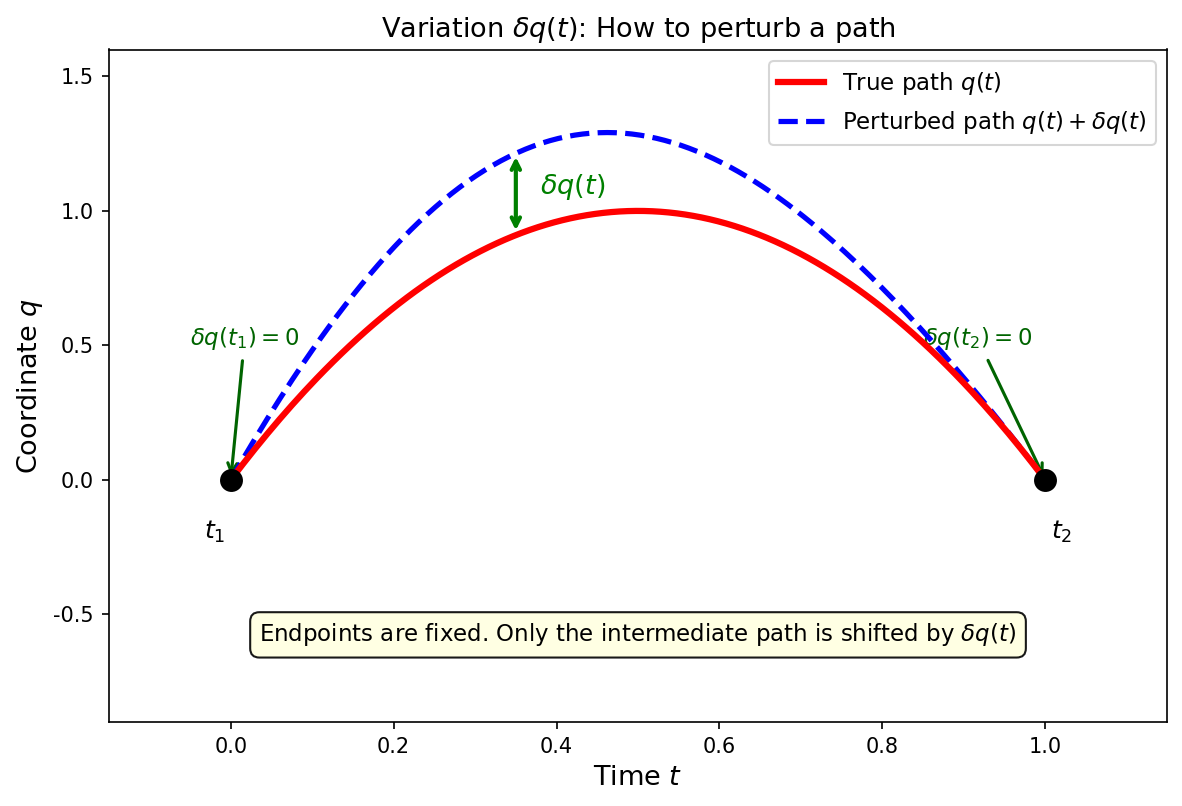
Fig. 1.13: Image of the variation \(\delta q(t)\). The solid red line is the actual path \(q(t)\), the dashed blue line is the perturbed path \(q(t) + \delta q(t)\). The endpoints are fixed (\(\delta q(t_1) = \delta q(t_2) = 0\)), and only the intermediate path is shifted by \(\delta q(t)\).
🔵 Kai: The \(\delta\) in \(\delta q\)—is that different from the ordinary differential \(d\)?
🟡 Lina: Good question. \(dq\) is "the change in \(q\) when you shift time slightly along the same path." \(\delta q\) is "the change when you shift to a different path at the same time." In other words, \(d\) is a shift in the time direction, and \(\delta\) is a shift in path space.
⚪ Mei: Keeping time \(t\) fixed, "if we had taken a different path, by how much would \(q\) differ"—that's \(\delta q(t)\).
🟡 Lina: Right. And the endpoints are fixed—we don't change the departure or arrival:
🔵 Kai: The start and end points stay the same, but we shift only the intermediate path slightly.
🟡 Lina: Exactly. Now let's calculate how much the action \(S\) changes when the path is shifted \(q \to q + \delta q\). This change \(\delta S\) is called the variation. Read as "delta S."
🔵 Kai: How do you calculate \(\delta S\)?
🟡 Lina: Recall that \(L(q, \dot{q}, t)\) is a two-variable function of \(q\) and \(\dot{q}\). Shifting the path \(q \to q + \delta q\) also changes the velocity. The velocity of the new path is \(\frac{d}{dt}(q + \delta q) = \dot{q} + \frac{d}{dt}(\delta q)\), so the velocity shift is:
That is, "the velocity of the shifted path" minus "the velocity of the original path." We just used linearity of differentiation (\((f+g)' = f' + g'\)).
⚪ Mei: "The rate of change of the shift \(\delta q\)" is \(\delta\dot{q}\). If the shift varies with time, the velocity shift varies with time too.
🟡 Lina: Right. Now let's compute the change in action. The action after shifting is \(S[q + \delta q] = \int_{t_1}^{t_2} L(q + \delta q,\, \dot{q} + \delta\dot{q},\, t)\, dt\). The change is:
🟡 Lina: Here, since \(\delta q\) is a "small" shift, we use the two-variable version of the approximation \(f(x + \Delta x) \approx f(x) + f'(x)\,\Delta x\) from high school. The one-variable case was "approximating by the tangent line." The two-variable case uses the same idea—in one variable it was "tangent line approximation," and in two variables it's "tangent plane approximation." The graph of a two-variable function \(f(a, b)\) is a surface in 3D space (with \(a\)-axis, \(b\)-axis, and \(f\)-axis). The flat surface tangent to that surface is the tangent plane. For a two-variable function \(f(a, b)\) when \(a \to a + \Delta a\), \(b \to b + \Delta b\):
This is an approximation up to first order (first power) in \(\Delta a\), \(\Delta b\). Second-order and higher terms like \(\Delta a \cdot \Delta b\) or \((\Delta a)^2\) are negligible when the shifts are sufficiently small. For example, if \(\Delta a = 0.01\) then \((\Delta a)^2 = 0.0001\), which is 1/100th of \(\Delta a\) itself—the smaller the shift, the more rapidly higher-order terms shrink compared to first-order terms. In the calculus of variations, we consider the limit of making \(\delta q\) smaller and smaller, so second-order and higher terms become negligible compared to first-order terms, and only the first-order terms determine the stationarity condition. This is exactly the same reasoning as when in high school we used "\(f(x+\Delta x) \approx f(x) + f'(x)\Delta x\)" to find the extremum condition \(f'(x) = 0\).
🔵 Kai: You add "slope × shift" in each variable direction. It's like extending the one-variable \(f'(x)\,\Delta x\) to two directions.
🟡 Lina: Let me show why simple addition works. First fix \(b\) and move only \(a\): the one-variable approximation gives \(f(a + \Delta a, b) \approx f(a, b) + \frac{\partial f}{\partial a}\Delta a\). Then from this state, move \(b\): \(f(a + \Delta a, b + \Delta b) \approx f(a + \Delta a, b) + \frac{\partial f}{\partial b}\Delta b\). Combining the two gives \(f(a, b) + \frac{\partial f}{\partial a}\Delta a + \frac{\partial f}{\partial b}\Delta b\). (In the second step, the point where the partial derivative is evaluated shifts slightly from \((a, b)\) to \((a + \Delta a, b)\), but the effect on the result is only a \(\Delta a \cdot \Delta b\) second-order term, negligible in first-order approximation.) Reversing the order gives the same result. For those who want to verify with a concrete example, see Problem B-8. Basic Calculations of Partial Derivatives.
🔵 Kai: But is it really OK to "ignore second order and higher"? Infinitely small but not zero—doesn't that cause issues?
🟡 Lina: Good question. In high school you learned "the condition for an extremum is \(f'(x) = 0\)." That meant "since \(f(x + \Delta x) - f(x) \approx f'(x)\,\Delta x\), if the first-order change is zero, the value doesn't change (at first order) whichever way you shift." The second-order term \(\frac{1}{2}f''(x)(\Delta x)^2\) is used to determine maximum vs. minimum, but to determine the location of the extremum, the first-order condition alone suffices. The calculus of variations works exactly the same way. Expand \(\delta S\) in powers of \(\delta q\) and extract only the first-order term. "The first-order term in \(\delta q\) equals zero" is the stationarity condition, and this alone determines the equation of motion. Higher-order terms are a factor of \(\delta q\) smaller than first-order terms when \(\delta q\) is small, so they don't affect finding the stationary point. This has the same structure as \(\lim_{\Delta x \to 0} \frac{f(x+\Delta x) - f(x) - f'(x)\Delta x}{\Delta x} = 0\) in the definition of the derivative—the "remainder" in the numerator approaches zero faster than \(\Delta x\), so even dividing by \(\Delta x\) gives zero.
🔵 Kai: Ah, the same idea as the definition of the derivative. "The first-order condition determines the extremum location"—and we're doing that for paths instead of functions.
🟡 Lina: Right. Applying to \(L\):
Subtracting the original \(L\):
⚪ Mei: The first term is "slope in the \(q\) direction × shift in \(q\)," the second is "slope in the \(\dot{q}\) direction × shift in \(\dot{q}\)." They separate cleanly.
🟡 Lina: Here there's one problem. The second term contains \(\delta\dot{q} = \frac{d}{dt}(\delta q)\). We want to eventually get everything in terms of "\(\delta q\) alone," but the time derivative of \(\delta q\) is mixed in. We need to deal with that.
🔵 Kai: How do you do that?
🟡 Lina: This is where we use integration by parts. Remember the product rule from Math III?
🔵 Kai: \((fg)' = f'g + fg'\), right.
🟡 Lina: Rearranging gives \(fg' = (fg)' - f'g\). Integrating both sides from \(t_1\) to \(t_2\):
This is the integration by parts formula. It "transfers the integration of \(g'\) to \(g\), while instead differentiating \(f\)."
🟡 Lina: Applying to our problem. In the formula \(\int f\,g'\,dt = [fg] - \int f'\,g\,dt\), set \(f = \frac{\partial L}{\partial \dot{q}}\), \(g = \delta q\) (so \(g' = \frac{d(\delta q)}{dt}\), \(f' = \frac{d}{dt}\frac{\partial L}{\partial \dot{q}}\)):
🔵 Kai: In the left side, "the derivative of \(\delta q\)" has become just "\(\delta q\) itself" on the right side! Instead, \(\frac{\partial L}{\partial \dot{q}}\) got differentiated.
🟡 Lina: Right. The derivative was "pushed onto the other party." Now look at the first term on the right—the boundary term. Since \(\delta q(t_1) = 0\) and \(\delta q(t_2) = 0\) (fixed endpoints):
⚪ Mei: Thanks to fixing the endpoints, the boundary term vanishes cleanly.
🟡 Lina: Now the second term is reorganized. Substituting back into the original \(\delta S\):
🔵 Kai: Ah, we factored out \(\delta q\)! The integrand is now in the form "(something) \(\times\,\delta q\)." But why did we want this form? What does factoring it out tell us?
🟡 Lina: Good question. The principle of least action requires "\(\delta S = 0\)"—as I said, this is the stationarity condition (first-order change is zero). That is:
Moreover, this must hold for any choice of shift \(\delta q(t)\).
🔵 Kai: "For any \(\delta q\)"—but why does that let us conclude the thing in parentheses is zero?
🟡 Lina: Think about it by contradiction. Suppose the expression in parentheses were nonzero at some time \(t^*\)—say positive. Since it's a continuous function, it stays positive near \(t^*\). Now choose a \(\delta q\) that is positive only near \(t^*\) and zero elsewhere—then what?
🔵 Kai: Ah, positive × positive = positive, so the integral over that part is positive. Everything else is zero, so the whole thing isn't zero either...!
🟡 Lina: Right. \(\delta S \neq 0\), contradicting "\(\delta S = 0\) for any \(\delta q\)." Therefore the expression in parentheses must be zero at all times:
🔵 Kai: ...But Professor, looking at this equation alone, I can't see how it's the same as \(F = ma\). What does \(\frac{d}{dt}\frac{\partial L}{\partial \dot{q}}\) represent?
🟡 Lina: This is the Euler-Lagrange equation. It looks completely different from \(F = ma\), right? But I'm about to substitute a specific \(L\) to reproduce the same result, and then the meaning of each term will become clear.
🟡 Lina: By the way, for multiple degrees of freedom (coordinates \(q_1, q_2, \ldots, q_n\)), the same form of equation holds independently for each coordinate \(q_i\):
But let's first confirm that \(F = ma\) emerges from a single degree of freedom.
✅ Comprehension Check: What is the difference between the variation \(\delta q(t)\) and the ordinary differential \(dq\)?
Answer
\(dq\) is the change in \(q\) when shifting time slightly along the same path. \(\delta q\) is the change when shifting to a different path at the same time. The condition \(\delta q(t_1) = \delta q(t_2) = 0\) (fixed endpoints) is imposed.
✅ Comprehension Check: What is the purpose of using integration by parts in the derivation of the Euler-Lagrange equation?
Answer
To eliminate \(\delta\dot{q}\) (the time derivative of \(\delta q\)) from the integrand and organize everything into the form "(something) \(\times \delta q\)." Integration by parts pushes the derivative onto the \(\partial L/\partial \dot{q}\) side, and the endpoint-fixing condition eliminates the boundary term.
Recovery of Newton's Equation of Motion
🟡 Lina: Now let's confirm that the Euler-Lagrange equation reproduces Newton's \(F = ma\). For a particle of mass \(m\) moving in one dimension in a potential \(V(x)\):
🟡 Lina: Let's compute each term in the Euler-Lagrange equation. First, the partial derivative with respect to \(\dot{x}\):
This is nothing other than momentum \(p = m\dot{x}\). Next, the time derivative:
And the partial derivative with respect to \(x\):
🔵 Kai: \(\frac{\partial L}{\partial \dot{x}}\) is momentum, and \(\frac{d}{dt}\frac{\partial L}{\partial \dot{x}}\) is mass × acceleration—so the left side of the Euler-Lagrange equation is the "\(ma\)" part!
🟡 Lina: Substituting into the Euler-Lagrange equation:
Rearranging:
🔵 Kai: The right side \(-dV/dx\)... ah, we just learned \(\mathbf{g} = -\nabla\Phi\) for gravity. Same structure—"force is the slope of potential"—so \(-dV/dx\) is the force \(F\)?
🟡 Lina: Exactly. \(F = -dV/dx\) is the general relation "force acts in the direction of decreasing potential energy." The gravitational \(\mathbf{g} = -\nabla\Phi\) was a special case. So \(m\ddot{x} = F\)—Newton's equation of motion \(F = ma\) has been derived from the principle of least action.
⚪ Mei: The starting point is completely different—"look at the entire path and extremize the action"—yet we arrive at the same equation \(F = ma\). This confirms that the two formulations describe the same physics.
✅ Comprehension Check: When \(L = \frac{1}{2}m\dot{x}^2 - V(x)\), what does \(\partial L/\partial \dot{x}\) physically represent?
Answer
Momentum \(p = m\dot{x}\). Taking the partial derivative of the Lagrangian with respect to velocity \(\dot{x}\) yields momentum. In general, \(\partial L/\partial \dot{q}\) is defined as the generalized momentum (also called canonical momentum). In this case, it coincides with ordinary momentum \(m\dot{x}\).
🔵 Kai: But Professor, you said earlier "fix the start and end points." If you can't use it without knowing the endpoint, doesn't that mean you can't predict the future?
🟡 Lina: Good question. Actually, "fixing start and end points" is a mathematical technique for deriving the Euler-Lagrange equation—it doesn't mean "you can't use it physically without knowing the endpoint."
🔵 Kai: What do you mean?
🟡 Lina: The role of the principle of least action is to be a "device for deriving the correct equation of motion." The Euler-Lagrange equation that comes out of it is a universal differential equation independent of boundary conditions. When actually predicting the future, you solve this equation by supplying "initial position \(q(t_1)\) and initial velocity \(\dot{q}(t_1)\)"—exactly the same as solving \(F = ma\) with initial conditions.
⚪ Mei: So the principle of least action is "a principle for finding the correct equation," and the actual predictions are carried out by the Euler-Lagrange equation that emerges from it. "Fixing start and end points" is scaffolding for deriving the equation—once the derivation is done, you can take it down.
Example: Free Fall in a Gravitational Field
🟡 Lina: Let's do one more concrete example. Free fall with the \(y\)-axis pointing vertically upward. The potential energy at height \(y\) is \(V = mgy\), so:
Euler-Lagrange equation:
Substituting into the Euler-Lagrange equation \(\frac{d}{dt}\frac{\partial L}{\partial \dot{y}} - \frac{\partial L}{\partial y} = 0\):
⚪ Mei: Out comes uniformly accelerated motion \(\ddot{y} = -g\). That's Galileo's law of falling bodies itself.
Why the Principle of Least Action Matters
🔵 Kai: But Professor, if you get the same answer, what's the point of a different formulation?
🟡 Lina: Three reasons.
🟡 Lina: First, symmetries become visible. If the Lagrangian doesn't depend on time, energy is conserved; if it doesn't depend on spatial position, momentum is conserved—these "relationships between symmetries and conserved quantities" emerge automatically (Noether's theorem, reappearing in Ch. 15 the relationship between Killing vectors and conserved quantities).
🔵 Kai: "The Lagrangian doesn't depend on time"—what does that mean concretely?
🟡 Lina: Look at the free-fall Lagrangian \(L = \frac{1}{2}m\dot{y}^2 - mgy\). Since \(g\) is a constant, time \(t\) doesn't appear directly in this expression for \(L\)—"the form is the same whenever you do the experiment." Of course \(y\) and \(\dot{y}\) change with time, but that's "change along the path"; the functional form of \(L\) itself doesn't depend on \(t\). We write this as \(\partial L/\partial t = 0\). This means "differentiating with respect to the third input slot \(t\) in \(L(q, \dot{q}, t)\) gives zero"—the same idea as treating \(q\) and \(\dot{q}\) as independent variables earlier; we differentiate with respect to \(t\) while holding \(q\) and \(\dot{q}\) fixed. Since \(t\) doesn't explicitly appear in the formula for \(L\), it's naturally zero. We say there is "time-translation symmetry." In this case, the conserved energy is \(T + V = \frac{1}{2}m\dot{y}^2 + mgy\)—the Lagrangian is \(T - V\), but the conserved quantity that emerges is \(T + V\) (total energy). Even as speed increases during a fall, height decreases by the same amount, so the sum stays constant. Why \(\partial L/\partial t = 0\) implies this will be proved in Ch. 15 Killing vectors and conserved quantities, but for now remember "there's such a powerful theorem."
🔵 Kai: What is symmetry? I hear the word a lot, but what does it mean in physics?
🟡 Lina: In one phrase: "performing some operation doesn't change the physical laws (the form of the Lagrangian)." Let me summarize.
Symmetry — "Changing without changing"
In physics, "having a symmetry" means the physical laws remain unchanged under some operation.
Operation Name of symmetry Resulting conserved quantity Shift the experimental location Spatial translation symmetry Momentum Shift the experimental time Time translation symmetry Energy Rotate the experimental apparatus Rotational symmetry Angular momentum "For every symmetry, there's one conserved quantity"—this is Noether's theorem. It reappears as Ch. 15 the relationship between Killing vectors and conserved quantities, with Quantum Field Theory Ch. 3 the general proof.
Note: Symmetry is not "something nature must necessarily possess." It's verified in the form "if we assume this symmetry, results agree with experiment"—part of the hypothesis.
🔵 Kai: I see. So in the free-fall example, "the same \(\ddot{y} = -g\) whether you experiment in Tokyo or Osaka" is spatial translation symmetry... right? But the table says "momentum is conserved"—is momentum conserved in free fall? The velocity changes as it falls, right?
🟡 Lina: Good question. Let me clarify. Your intuition that "same laws in Tokyo or Osaka" is correct, and it is indeed a type of symmetry. But Noether's theorem's "symmetry → conserved quantity" is more specific. The point is "if the Lagrangian doesn't depend on some coordinate, momentum in that direction is conserved." For 1D free fall, \(L = \frac{1}{2}m\dot{y}^2 - mgy\) has \(y\) appearing in \(L\), so \(y\)-direction momentum is not conserved—consistent with your intuition. But consider throwing a ball at an angle. Including both horizontal \(x\) and vertical \(y\) directions: \(L = \frac{1}{2}m(\dot{x}^2 + \dot{y}^2) - mgy\) (we just added the \(x\)-direction contribution \(\frac{1}{2}m\dot{x}^2\) to kinetic energy). Looking at this expression, \(x\) (horizontal direction) doesn't explicitly appear in \(L\). So \(x \to x + \text{constant}\) doesn't change \(L\)—this is "spatial translation symmetry in the horizontal direction." By Noether's theorem, the corresponding conserved quantity is horizontal momentum \(m\dot{x}\). The constant horizontal velocity of a thrown ball is precisely this. Meanwhile, the \(mgy\) term breaks \(y\)-direction translation symmetry, and vertical momentum is not conserved (it accelerates due to gravity).
🔵 Kai: Ah, I see. "Same laws wherever you go" is the big picture, and "the Lagrangian doesn't contain \(x\) so \(x\)-direction momentum is conserved" is the specific statement—they're at different levels. The latter is much more concrete and tells you exactly which direction has a conserved quantity.
🟡 Lina: Exactly. Noether's theorem provides a one-to-one correspondence between "which symmetry corresponds to which conserved quantity." That's why it's powerful.
🟡 Lina: Second, it's coordinate-independent. If you write \(F = ma\) in components, in polar coordinates apparent terms like centrifugal and Coriolis forces appear, changing the equation's form. But the Euler-Lagrange equation maintains the same form \(\frac{d}{dt}\frac{\partial L}{\partial \dot{q}_i} - \frac{\partial L}{\partial q_i} = 0\) in any coordinates. In general relativity from Ch. 2 onward, coordinate-independent description becomes essentially important.
⚪ Mei: The fact that the "form" of the equation doesn't change under coordinate transformations will become essentially important when dealing with coordinate freedom in general relativity ahead.
🟡 Lina: Third, the extension to field theory is natural. If you extend the particle Lagrangian \(L(q, \dot{q})\) to a quantity called the "field Lagrangian density," the field equations of motion can be derived within the same framework. The notation and details are covered in Appendix C field theory, but what's important is that the procedure "write the Lagrangian and extremize the action" is exactly the same. The Ch. 14 Einstein equation and Ch. 24 variation of the Einstein-Hilbert action all stand on this principle.
🔵 Kai: So even in electromagnetism or general relativity, you write a Lagrangian and derive equations using the same procedure? Completely different physics yet the same method works... But why can nature always be described in the form "extremize the action"? Isn't that itself mysterious?
🟡 Lina: A deep question. Honestly, there's no ultimate answer to "why the principle of least action holds." However, all fundamental models in physics can be formulated by writing down a Lagrangian and extremizing the action—and the results agree with experiment. \(F = ma\) is specific to Newtonian mechanics, but the principle of least action serves as a "common language" across all fields. This is the tool we'll use from here on.
✅ Comprehension Check: State one of the three reasons mentioned in the text for why the principle of least action is superior to \(F = ma\).
Answer
(Any one of the following) (1) The relationship between symmetries and conserved quantities becomes automatically visible. (2) It's coordinate-independent. (3) Extension to field theory is natural.
✅ Comprehension Check: According to Noether's theorem, what is conserved when the Lagrangian does not explicitly depend on time (\(\partial L/\partial t = 0\))?
Answer
Energy is conserved. This is the conserved quantity corresponding to "time-translation symmetry" (the physical laws are the same whenever you do the experiment).
How Do You Find the Lagrangian?
🔵 Kai: But Professor, how do you find the Lagrangian? Did someone just decide "let's make it \(L = T - V\)"?
🟡 Lina: Good question. There are broadly two ways to find the Lagrangian. First, constrain it from symmetry. If you require "this system should have such-and-such symmetry," the form of the Lagrangian becomes quite restricted. Second, compare with experiment. Derive the equations of motion from a candidate Lagrangian and compare with experimental results. If they don't match, revise the Lagrangian.
⚪ Mei: So the Lagrangian itself is a "hypothesis."
🟡 Lina: Exactly. It's not an overstatement to say a physicist's job is "finding the correct Lagrangian." In Newtonian mechanics it's \(L = T - V\); in electromagnetism it's a different form; in general relativity it uses the scalar curvature \(R\) in the Einstein-Hilbert action. The forms differ, but the framework "write the Lagrangian and extremize the action" is common to all.
✅ Comprehension Check: How is the action \(S\) defined? What is the Lagrangian \(L\)?
Answer
\(S = \int_{t_1}^{t_2} L\, dt\). The Lagrangian is \(L = T - V\) (the difference between kinetic energy and potential energy).
✅ Comprehension Check: Write the Euler-Lagrange equation and verify that Newton's equation of motion follows from \(L = \frac{1}{2}m\dot{x}^2 - V(x)\).
Answer
Euler-Lagrange equation: \(\frac{d}{dt}\frac{\partial L}{\partial \dot{q}} - \frac{\partial L}{\partial q} = 0\). Substituting \(L = \frac{1}{2}m\dot{x}^2 - V(x)\) gives \(m\ddot{x} = -dV/dx\), i.e., \(F = ma\).
1.8 Chapter Summary
🟡 Lina: Let me organize today's content.
- We rewrote Newton's universal gravitation \(F = Gm_1m_2/r^2\) as a "field theory" using the gravitational field \(\mathbf{g} = -\nabla\Phi\) and gravitational potential \(\Phi\)
- The field equation determining the potential is the Poisson equation \(\nabla^2\Phi = 4\pi G\rho\)
- Success story: The discovery of Neptune—a quantitative prediction of Newton's model brilliantly confirmed
- Limitation ①: Mercury's perihelion precession—Newton's model prediction deviates from observation by 43 arcseconds per century
- Limitation ②: The Poisson equation has no time derivative, so gravitational changes propagate instantaneously—contradicting special relativity
- The principle of least action—defined the Lagrangian \(L = T - V\) and action \(S = \int L\,dt\), derived the Euler-Lagrange equation \(\frac{d}{dt}\frac{\partial L}{\partial \dot{q}} - \frac{\partial L}{\partial q} = 0\) from the stationarity condition \(\delta S = 0\) (not necessarily a "minimum" despite the historical name), and reproduced Newton's \(F = ma\). This framework will be used repeatedly in the Ch. 8 geodesic equation, Ch. 14 Einstein equation, and Appendix C field theory
🔵 Kai: Newton's model isn't "wrong"—it's "an approximation to a more accurate model."
🟡 Lina: Exactly. Today we saw the first concrete example of "models are hypotheses" from the Prologue.
Preview of Next Chapter
In Ch. 2 Blueprint for the Journey — Tensors and the Big Picture of the Einstein Equation, we'll spread out the overall design blueprint needed to go beyond Newton's limitations. We introduce tensors—tools for writing physical models in a form independent of coordinate systems—and survey how Einstein's gravitational model is structured around two pillars: "the geodesic equation that determines particle motion" and "the Einstein equation that determines the shape of spacetime." The detailed mathematical derivations proceed step by step from Ch. 3 onward, but first let's grasp "where we're heading."
References
- Hartle, J. B. (2003). Gravity: An Introduction to Einstein's General Relativity. Addison-Wesley. Ch. 1, Ch. 3.
- Tong, D. (2019). General Relativity. University of Cambridge Part II Mathematical Tripos. Ch. 1. http://www.damtp.cam.ac.uk/user/tong/gr.html
- 石井俊全 (2013).『一般相対性理論を一歩一歩数式で理解する』ベレ出版. 第 2 章「物理の準備」.
Feedback on this page
Let us know if something was unclear, incorrect, or could be improved.