Ch. 6 Solutions
← Back to problems | Back to chapter
Table of Contents
Basic
- B-1. Jacobian of 2D Polar Coordinates
- B-2. Inverse Metric in 3D Spherical Coordinates
- B-3. Matrix Representation of a General 2-Dimensional Metric
- B-4. Metric Tensor on a Sphere at a Specific Point
- B-5. Jacobian Matrix of a Linear Coordinate Transformation
- B-6. Application of the Metric Tensor Transformation Law
- B-7. Cartesian Components of Coordinate Basis Vectors
- B-8. Determinant of the Jacobian Matrix of the Inverse Transformation
Medium
- M-1. Coordinate Transformation \((u, v)\) and the Metric Tensor
- M-2. Derivation of the Line Element in Spherical Coordinates
- M-3. Metric Tensor in Parabolic Coordinates
- M-4. Proof of Symmetry of the Metric Tensor
- M-5. Metric and Flatness of a Cylindrical Surface
- M-6. Geometry of "Circles" on a Sphere
- M-7. Derivation of \(g'_{33}\) using the metric tensor transformation law
Advanced
Basic
B-1. Jacobian of 2D Polar Coordinates
Problem:
Find the determinant (Jacobian) \(\det J\) of the Jacobi matrix
for the transformation from 2D polar coordinates \((r, \theta)\) to Cartesian coordinates \((x, y)\).
Solution strategy: Directly compute the determinant of the Jacobian matrix.
The Jacobian matrix is:
Computing the determinant:
Verification: This is consistent with the Jacobian being \(r\) in the polar coordinate area element \(dA = r\,dr\,d\theta\). Furthermore, the transformation is non-singular for \(r > 0\) and degenerates at \(r = 0\) (the origin), which is geometrically correct.
B-2. Inverse Metric in 3D Spherical Coordinates
Problem:
From the line element in 3-dimensional spherical coordinates \((r, \theta, \varphi)\)
find the inverse matrix \(g^{ij}\) (inverse metric) of the metric tensor \(g_{ij}\).
Solution strategy: Since the metric tensor is a diagonal matrix, the inverse is obtained by taking the reciprocal of each diagonal component.
The metric tensor is:
Since the inverse of a diagonal matrix has reciprocals of each diagonal component:
Verification: We confirm that \(g_{ij}\,g^{jk} = \delta_i^k\). For example, the \((2,2)\) component: \(r^2 \cdot \dfrac{1}{r^2} = 1\). The \((3,3)\) component: \(r^2\sin^2\theta \cdot \dfrac{1}{r^2\sin^2\theta} = 1\). All off-diagonal components are 0. This indeed gives the identity matrix. ✓
B-3. Matrix Representation of a General 2-Dimensional Metric
Problem:
Given a metric in 2-dimensional coordinates \((u, v)\):
Write the metric tensor \(g_{ij}\) in \(2 \times 2\) matrix form.
Solution strategy: Expand \(ds^2 = g_{ij}\,du^i\,du^j\) and compare coefficients.
Expanding the line element:
Using the symmetry of the metric tensor \(g_{12} = g_{21}\), the coefficient of the cross term is \(2g_{12}\).
Comparing with the given line element:
- \(g_{11} = 1 + u^2\)
- \(2g_{12} = 2uv \implies g_{12} = uv\)
- \(g_{22} = 1 + v^2\)
Verification: The determinant \(\det g = (1+u^2)(1+v^2) - u^2v^2 = 1 + u^2 + v^2 > 0\), so the matrix is positive definite, which is consistent with a Riemannian metric. ✓
B-4. Metric Tensor on a Sphere at a Specific Point
Problem:
For the metric on a sphere of radius \(a\)
write down the explicit components of the metric tensor \(g_{ij}\) at the point \((\theta, \varphi) = (\pi/3,\, 0)\).
Solution strategy: Substitute \(\theta = \pi/3\) into the metric tensor components.
The metric tensor of the sphere is:
At \(\theta = \pi/3\), since \(\sin(\pi/3) = \dfrac{\sqrt{3}}{2}\), we have \(\sin^2(\pi/3) = \dfrac{3}{4}\).
Verification: At \(\theta = \pi/2\) (the equator), \(g_{22} = a^2\) is maximized; at \(\theta = 0\) (the north pole), \(g_{22} = 0\) and the metric degenerates. Since \(\theta = \pi/3\) lies between the equator and the north pole, \(g_{22} = \frac{3}{4}a^2\) falls between \(0\) and \(a^2\), which is consistent. ✓
B-5. Jacobian Matrix of a Linear Coordinate Transformation
Problem:
In 2 dimensions, a transformation from coordinates \((x^1, x^2) = (x, y)\) to \((u^1, u^2) = (u, v)\) is given by
Find the Jacobian matrix \(\dfrac{\partial x^i}{\partial u^j}\).
Solution strategy: Compute each partial derivative directly.
From \(x = u + v\), \(y = u - v\):
Verification: \(\det J = 1 \cdot (-1) - 1 \cdot 1 = -2 \neq 0\), so it is nonsingular. This is consistent with the existence of the inverse transformation \(u = \frac{x+y}{2}\), \(v = \frac{x-y}{2}\). ✓
B-6. Application of the Metric Tensor Transformation Law
Problem:
For the coordinate transformation in Problem B-5. Jacobian Matrix of a Linear Coordinate Transformation, use the metric tensor transformation law
to find the metric tensor \(g'_{kl}\) in the new coordinates \((u, v)\), starting from the Cartesian metric \(g_{ij} = \delta_{ij}\). Write the result in matrix form.
Solution strategy: Compute \(g' = J^T g\,J = J^T J\) (since \(g = \delta_{ij}\)).
Computing each component:
- \((1,1)\): \(1 \cdot 1 + 1 \cdot 1 = 2\)
- \((1,2)\): \(1 \cdot 1 + 1 \cdot (-1) = 0\)
- \((2,1)\): \(1 \cdot 1 + (-1) \cdot 1 = 0\)
- \((2,2)\): \(1 \cdot 1 + (-1)(-1) = 2\)
That is, the line element becomes \(ds^2 = 2\,du^2 + 2\,dv^2\).
Verification: Confirm by direct substitution. From \(dx = du + dv\), \(dy = du - dv\):
B-7. Cartesian Components of Coordinate Basis Vectors
Problem:
For the coordinate basis vector \(\boldsymbol{e}_\theta\) in 2-dimensional polar coordinates, find the Cartesian components \((\boldsymbol{e}_\theta)^x\) and \((\boldsymbol{e}_\theta)^y\) at the point \(r = 3\), \(\theta = \pi/4\).
Solution Strategy: Find the Cartesian components of \(\boldsymbol{e}_\theta\) using partial derivatives, then substitute specific values.
From the definition of coordinate basis vectors:
From \(x = r\cos\theta\), \(y = r\sin\theta\):
Substituting \(r = 3\), \(\theta = \pi/4\), and using \(\sin(\pi/4) = \cos(\pi/4) = \dfrac{\sqrt{2}}{2}\):
Verification: The squared magnitude of \(\boldsymbol{e}_\theta\) is \(|\boldsymbol{e}_\theta|^2 = \left(\frac{3\sqrt{2}}{2}\right)^2 + \left(\frac{3\sqrt{2}}{2}\right)^2 = \frac{18}{4} + \frac{18}{4} = 9 = r^2\). This is consistent with the metric tensor component \(g_{\theta\theta} = r^2 = 9\). ✓
B-8. Determinant of the Jacobian Matrix of the Inverse Transformation
Problem:
In 2-dimensional polar coordinates, find the determinant \(\det \tilde{J}\) of the Jacobian matrix of the inverse transformation
and verify its relationship with \(\det J\) obtained in Problem B-1. Jacobian of 2D Polar Coordinates.
Solution strategy: Derive the determinant relationship from the relation \(J\tilde{J} = I\).
Taking the determinant of both sides of \(J\tilde{J} = I\):
From Problem B-1. Jacobian of 2D Polar Coordinates, \(\det J = r\), so:
\(\det J\) and \(\det \tilde{J}\) are reciprocals of each other.
Verification: We confirm this by directly using the Jacobian matrix of the inverse transformation. From the main text:
Medium
M-1. Coordinate Transformation \((u, v)\) and the Metric Tensor
Problem:
Reference figure: Figure 5.1: Cartesian and Polar Coordinates
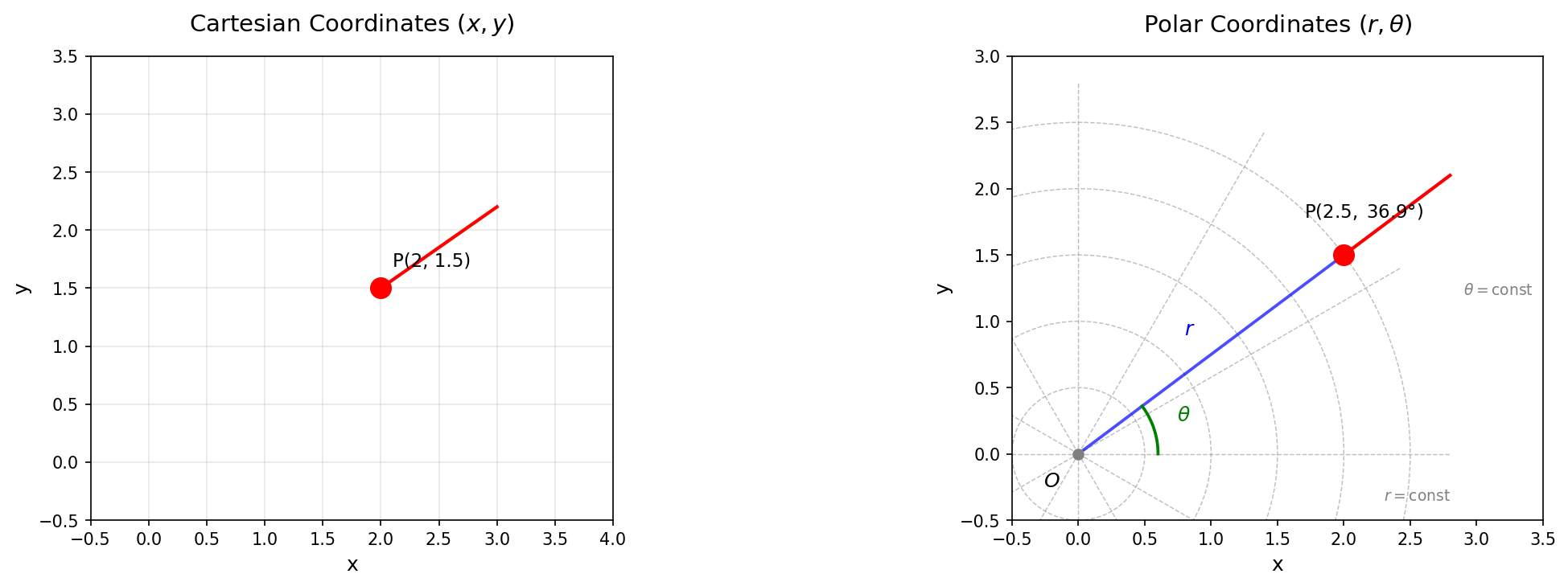
Consider the coordinate transformation \(u = x + y\), \(v = x - y\) in a 2-dimensional plane.
(a) Find the Jacobian matrix \(\dfrac{\partial(x, y)}{\partial(u, v)}\).
(b) Using the transformation law, find the metric tensor \(g'_{ij}\) in this coordinate system.
(c) Rewrite \(ds^2 = dx^2 + dy^2\) in these coordinates and verify that it agrees with the result of (b).
Solution strategy: Find the Jacobian matrix of the inverse transformation, derive the metric tensor using the transformation law, and verify by direct substitution.
(a) Jacobian matrix \(\partial(x, y)/\partial(u, v)\):
We find the inverse of the coordinate transformation \(u = x + y\), \(v = x - y\). Solving the system of equations gives:
The Jacobian matrix is:
(b) Derivation of the metric tensor \(g'_{ij}\) using the transformation law:
We use the transformation law \(g'_{kl} = \dfrac{\partial x^i}{\partial u^k}\dfrac{\partial x^j}{\partial u^l}\,g_{ij}\). Since the metric in the original coordinates is \(g_{ij} = \delta_{ij}\) (Cartesian coordinates), we simply compute \(g' = J^T J\).
Computing each component:
-
\((1,1)\): \(\dfrac{1}{2}\cdot\dfrac{1}{2} + \dfrac{1}{2}\cdot\dfrac{1}{2} = \dfrac{1}{4} + \dfrac{1}{4} = \dfrac{1}{2}\)
-
\((1,2)\): \(\dfrac{1}{2}\cdot\dfrac{1}{2} + \dfrac{1}{2}\cdot\left(-\dfrac{1}{2}\right) = \dfrac{1}{4} - \dfrac{1}{4} = 0\)
-
\((2,1)\): \(\dfrac{1}{2}\cdot\dfrac{1}{2} + \left(-\dfrac{1}{2}\right)\cdot\dfrac{1}{2} = \dfrac{1}{4} - \dfrac{1}{4} = 0\)
-
\((2,2)\): \(\dfrac{1}{2}\cdot\dfrac{1}{2} + \left(-\dfrac{1}{2}\right)\left(-\dfrac{1}{2}\right) = \dfrac{1}{4} + \dfrac{1}{4} = \dfrac{1}{2}\)
(c) Verification by direct substitution:
From \(x = (u+v)/2\), \(y = (u-v)/2\), we have:
Substituting into \(ds^2 = dx^2 + dy^2\):
This is in perfect agreement with the metric tensor \(g'_{ij} = \text{diag}(1/2,\, 1/2)\) obtained in (b). ✓
Consistency check: \(\det J = \dfrac{1}{2}\cdot\left(-\dfrac{1}{2}\right) - \dfrac{1}{2}\cdot\dfrac{1}{2} = -\dfrac{1}{2} \neq 0\), so the matrix is non-singular. The relation \(\det g' = 1/4 = (\det J)^2\) is also consistent. Since the metric is diagonal and constant, this coordinate system is orthogonal, and the space is flat (consistent with the discussion in Problem M-5. Metric and Flatness of a Cylindrical Surface). ✓
M-2. Derivation of the Line Element in Spherical Coordinates
Problem:
Derive the line element in 3-dimensional spherical coordinates \((r, \theta, \varphi)\)
from the Cartesian line element \(ds^2 = dx^2 + dy^2 + dz^2\) and the coordinate transformation
Express the total differentials \(dx\), \(dy\), \(dz\) in terms of \((dr, d\theta, d\varphi)\), substitute them in, and show the entire process of simplification.
Solution strategy: Find the total differentials of \(x = r\sin\theta\cos\varphi\), \(y = r\sin\theta\sin\varphi\), \(z = r\cos\theta\), and substitute into \(ds^2 = dx^2 + dy^2 + dz^2\).
Computing the total differentials:
Computing \(dx\):
Computing \(dy\):
Computing \(dz\):
Expanding \(dx^2\):
Expanding \(dy^2\):
Expanding \(dz^2\):
Summing the terms:
Coefficient of \(dr^2\):
Coefficient of \(d\theta^2\):
Coefficient of \(d\varphi^2\):
Coefficient of \(dr\,d\theta\):
Coefficient of \(dr\,d\varphi\):
Coefficient of \(d\theta\,d\varphi\):
Final result:
All cross terms vanish:
Verification:
- Restricting to \(\theta = \pi/2\) (the \(xy\) plane) gives \(ds^2 = dr^2 + r^2\,d\varphi^2\), which matches the line element in 2D polar coordinates. ✓
- Dimensional analysis: each term has dimensions of [length]\(^2\). ✓
M-3. Metric Tensor in Parabolic Coordinates
Problem:
Two-dimensional parabolic coordinates \((\sigma, \tau)\) are defined by
(a) Find the Jacobian matrix \(\dfrac{\partial x^i}{\partial u^j}\), where \((u^1, u^2) = (\sigma, \tau)\).
(b) Using the transformation law for the metric tensor, derive the metric tensor \(g'_{kl}\) in parabolic coordinates, and express the line element \(ds^2\) in terms of \((\sigma, \tau)\).
(a) Jacobian Matrix:
From \(x = \sigma\tau\), \(y = \frac{1}{2}(\tau^2 - \sigma^2)\):
(b) Derivation of the Metric Tensor:
Computing \(g' = J^T J\):
Each component:
- \((1,1)\): \(\tau^2 + \sigma^2\)
- \((1,2)\): \(\tau\sigma - \sigma\tau = 0\)
- \((2,1)\): \(\sigma\tau - \tau\sigma = 0\)
- \((2,2)\): \(\sigma^2 + \tau^2\)
Therefore the line element is:
Verification: The metric takes the conformally flat form \(ds^2 = \Omega^2(d\sigma^2 + d\tau^2)\). This means that parabolic coordinates form an orthogonal coordinate system (\(g_{12} = 0\)), which is consistent with the properties of conformal mappings.
Furthermore, we can verify that \(\det J = \tau^2 + \sigma^2\) and \(\det g' = (\sigma^2 + \tau^2)^2 = (\det J)^2\) holds. ✓
M-4. Proof of Symmetry of the Metric Tensor
Problem:
Reference figure: Figure 5.2: Metric of a sphere
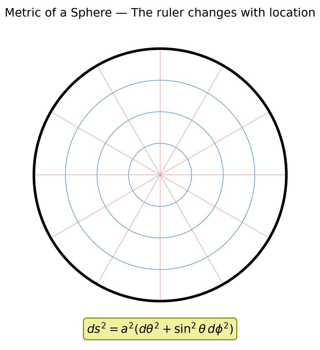
Given the transformation law for the metric tensor
show that the metric tensor is a symmetric tensor, i.e., \(g'_{kl} = g'_{lk}\), assuming symmetry in the original coordinate system \(g_{ij} = g_{ji}\).
Solution Strategy: Swap indices on the right-hand side of the transformation law and use \(g_{ij} = g_{ji}\).
The transformation law for the metric tensor is:
Writing out \(g'_{lk}\):
Relabeling the dummy indices \(i\) and \(j\) on the right-hand side (simply renaming the summation indices does not change the value):
Using \(g_{ji} = g_{ij}\) (the symmetry assumption in the original coordinate system):
Therefore, if the metric tensor is symmetric in the original coordinate system, symmetry is preserved under any coordinate transformation. \(\blacksquare\)
Verification: We confirm using the concrete example in Problem B-6. Application of the Metric Tensor Transformation Law. \(g'_{kl} = \begin{pmatrix} 2 & 0 \\ 0 & 2 \end{pmatrix}\) is clearly symmetric. In the parabolic coordinates of Problem M-3. Metric Tensor in Parabolic Coordinates, \(g'_{12} = g'_{21} = 0\), which is also symmetric. ✓
M-5. Metric and Flatness of a Cylindrical Surface
Problem:
When describing a cylindrical surface of radius \(a\) using coordinates \((\varphi, z)\) (where \(\varphi\) is the circumferential angle and \(z\) is the height), the line element is
(a) Write the metric tensor \(g_{ij}\) in matrix form.
(b) The components of the metric tensor for the cylindrical surface are constants that do not depend on the coordinates. Contrast this with the fact that the metric tensor components of a sphere depend on \(\theta\), and discuss whether the claim "constant metric tensor components ⇒ the space is flat" is correct, based on the content of this chapter.
(a) Matrix Representation of the Metric Tensor:
From the line element \(ds^2 = a^2\,d\varphi^2 + dz^2\):
(b) Relationship Between Constant Metric Tensor and Flatness:
Conclusion: The statement "metric tensor components are constant ⇒ the space is flat" is correct.
The reasoning is given below.
The cylinder surface is flat:
A cylinder surface can be made by rolling up a sheet of paper. The rolling operation does not change any distance relationships on the paper (no stretching or compression), so the intrinsic geometry of the cylinder surface is the same as that of a flat plane. Indeed, performing the coordinate transformation \(s = a\varphi\):
which is precisely the line element of a plane in Cartesian coordinates.
Meaning of constant metric tensor components:
When all components of the metric tensor are constant, the metric can be transformed to \(\delta_{ij}\) (the identity matrix) by a coordinate transformation (a linear transformation with a constant matrix). Specifically, if \(g_{ij}\) is a positive-definite symmetric constant matrix, then there exists an appropriate constant matrix \(A\) such that \(A^T g A = I\). The coordinates after this transformation are Cartesian coordinates themselves, and the space is flat.
Contrast with the sphere:
The metric tensor of a sphere \(g_{ij} = \begin{pmatrix} a^2 & 0 \\ 0 & a^2\sin^2\theta \end{pmatrix}\) depends on \(\theta\). However, as discussed in this chapter, the mere fact that the metric tensor depends on coordinates does not imply that the space is curved (even in polar coordinates on a flat plane, \(g_{22} = r^2\) depends on coordinates). Whether a space is truly curved is determined by whether the metric tensor can be made constant (or equal to \(\delta_{ij}\)) through a coordinate transformation. In the case of the sphere, no coordinate transformation can make the metric tensor constant, which reflects the fact that the sphere is intrinsically curved (strictly speaking, this is determined by the Riemann curvature tensor).
However, the converse does not hold (even in a flat space, the metric tensor depends on coordinates if curvilinear coordinates are used).
M-6. Geometry of "Circles" on a Sphere
Problem:
On a sphere of radius \(a\), consider a "circle" centered at the north pole (\(\theta = 0\)), defined by the line \(\theta = \theta_0\) = constant.
(a) Find the circumference \(C\) of this circle using the metric of the sphere \(ds^2 = a^2\,d\theta^2 + a^2\sin^2\theta\,d\varphi^2\).
(b) Find the distance \(r\) along the sphere's surface from the north pole to this circle (the distance along a meridian with \(\varphi\) = constant).
(c) Calculate \(C/(2\pi r)\) and verify that it becomes less than 1 as \(\theta_0\) increases. This is a manifestation of the sphere having positive curvature.
Strategy: Use the metric of the sphere \(ds^2 = a^2(d\theta^2 + \sin^2\theta\,d\varphi^2)\) to calculate the circumference and distance.
(a) Calculating the circumference \(C\):
On the line \(\theta = \theta_0\) = constant, \(d\theta = 0\), so the line element is
Integrating \(\varphi\) from \(0\) to \(2\pi\),
(b) Distance \(r\) from the north pole along the sphere:
The distance along the sphere from the north pole (\(\theta = 0\)) to the line \(\theta = \theta_0\) is measured along a great circle with \(\varphi\) = constant. Since \(d\varphi = 0\),
Integrating \(\theta\) from \(0\) to \(\theta_0\),
(c) Calculating \(C/(2\pi r)\):
Verifying that this becomes less than 1 as \(\theta_0\) increases:
For \(\theta_0 > 0\), the inequality \(\sin\theta_0 < \theta_0\) holds (\(\sin x < x\) for \(x > 0\)). Therefore,
In the limit \(\theta_0 \to 0\), \(\sin\theta_0/\theta_0 \to 1\), so for sufficiently small circles the flat-space ratio \(C = 2\pi r\) is recovered. As \(\theta_0\) increases, the ratio decreases from 1; at \(\theta_0 = \pi/2\) (the equator), \(C/(2\pi r) = \sin(\pi/2)/(\pi/2) = 2/\pi \approx 0.637\).
Physical interpretation: In flat space, the ratio of circumference to radius is always \(C = 2\pi r\) (\(C/(2\pi r) = 1\)). The fact that this ratio is less than 1 on the sphere is a direct manifestation of the sphere's positive curvature. In a space with positive curvature, the circumference is "deficient" relative to the distance from the center—it is shorter than in the flat-space case. This is an intrinsic geometric property of the sphere, a quantity that can be calculated directly from the metric tensor.
Consistency check: At \(\theta_0 = \pi\) (the "circle" enclosing the south pole), \(C = 2\pi a\sin\pi = 0\) and \(r = a\pi\). Since the south pole is a single point, the circumference should indeed be zero. ✓
Taylor expanding for \(\theta_0 \to 0\) gives \(\sin\theta_0 \approx \theta_0 - \theta_0^3/6\), so \(C/(2\pi r) \approx 1 - \theta_0^2/6\). It is known that for a sphere with curvature \(K = 1/a^2\), the relation \(C/(2\pi r) \approx 1 - Kr^2/6\) holds. Substituting \(r = a\theta_0\) gives \(1 - (1/a^2)(a\theta_0)^2/6 = 1 - \theta_0^2/6\), which agrees. ✓
M-7. Derivation of \(g'_{33}\) using the metric tensor transformation law
Problem:
Using the metric tensor transformation law
derive the 3-dimensional spherical coordinate metric component \(g'_{33} = r^2\sin^2\theta\) from the Cartesian metric \(g_{ij} = \delta_{ij}\). (Hint: Use \(\dfrac{\partial x}{\partial \varphi} = -r\sin\theta\sin\varphi\), \(\dfrac{\partial y}{\partial \varphi} = r\sin\theta\cos\varphi\), \(\dfrac{\partial z}{\partial \varphi} = 0\).)
Solution Strategy: Starting from the relationship between spherical coordinates \((r, \theta, \varphi)\) and Cartesian coordinates \((x, y, z)\), derive \(g'_{33} = r^2\sin^2\theta\) using the transformation law.
Calculation:
Coordinate correspondence: let \(u^1 = r\), \(u^2 = \theta\), \(u^3 = \varphi\), and \(x^1 = x\), \(x^2 = y\), \(x^3 = z\).
The transformation law gives:
(Since \(g_{ij} = \delta_{ij}\), only the \(i = j\) terms survive.)
From the coordinate transformation \(x = r\sin\theta\cos\varphi\), \(y = r\sin\theta\sin\varphi\), \(z = r\cos\theta\), we compute each partial derivative:
Substituting into the transformation law:
This agrees with the known value of the \((3,3)\) component of the metric tensor in spherical coordinates.
Verification: This matches the coefficient of \(d\varphi^2\) in the spherical coordinate line element \(ds^2 = dr^2 + r^2\,d\theta^2 + r^2\sin^2\theta\,d\varphi^2\) derived by direct substitution in Problem M-2. Derivation of the Line Element in Spherical Coordinates. ✓
At \(\theta = \pi/2\) (the equatorial plane), \(g'_{33} = r^2\), which reduces to \(g_{\varphi\varphi} = r^2\) for 2-dimensional polar coordinates. ✓
At \(\theta = 0\) (on the \(z\)-axis), \(g'_{33} = 0\), which is consistent with the fact that the \(\varphi\) coordinate degenerates (changes in \(\varphi\) do not contribute to distance on the \(z\)-axis). ✓
Advanced
A-1. Metric Tensor in General Curvilinear Coordinates
Problem:
Consider "general curvilinear coordinates" \((u^1, u^2)\) on a 2-dimensional plane:
where \(f\) and \(g\) are sufficiently smooth functions and the Jacobian matrix is non-singular.
(a) Express the metric tensor \(g_{ij}\) in these coordinates in terms of partial derivatives of \(f\) and \(g\).
(b) Write down the condition for the coordinate basis vectors \(\boldsymbol{e}_1\) and \(\boldsymbol{e}_2\) to be orthogonal (\(g_{12} = 0\)) using partial derivatives of \(f\) and \(g\).
(c) For polar coordinates and parabolic coordinates (see Problem M-3. Metric Tensor in Parabolic Coordinates), verify whether the orthogonality condition from (b) is satisfied in each case.
(a) Derivation of the Metric Tensor:
For \(x = f(u^1, u^2)\), \(y = g(u^1, u^2)\), we transform the Cartesian metric \(ds^2 = dx^2 + dy^2\).
The total differentials are:
From \(ds^2 = dx^2 + dy^2 = g_{ij}\,du^i\,du^j\):
Using the shorthand notation \(f_i \equiv \dfrac{\partial f}{\partial u^i}\), \(g_i \equiv \dfrac{\partial g}{\partial u^i}\):
Writing out the components explicitly:
(b) Orthogonality Condition:
The condition for the coordinate basis vectors to be orthogonal, \(g_{12} = 0\), is:
This means that the inner product of the two coordinate basis vectors \(\boldsymbol{e}_1 = (f_1, g_1)\) and \(\boldsymbol{e}_2 = (f_2, g_2)\) is zero.
(c) Verification with Specific Examples:
Polar coordinates \((u^1, u^2) = (r, \theta)\):
From \(f = r\cos\theta\), \(g = r\sin\theta\):
Checking the orthogonality condition:
Polar coordinates form an orthogonal coordinate system.
Parabolic coordinates \((u^1, u^2) = (\sigma, \tau)\):
From \(f = \sigma\tau\), \(g = \frac{1}{2}(\tau^2 - \sigma^2)\):
Checking the orthogonality condition:
Parabolic coordinates also form an orthogonal coordinate system.
Verification: This is consistent with the fact that the metric tensor for parabolic coordinates obtained in Problem M-3. Metric Tensor in Parabolic Coordinates is a diagonal matrix (\(g_{12} = 0\)). The polar coordinate metric \(ds^2 = dr^2 + r^2\,d\theta^2\) is also diagonal, which is consistent. ✓
A-2. Rindler Coordinates
Problem:
Reference figure: Figure 2.1: Light cones and spacetime diagrams (Chapters 3–4)
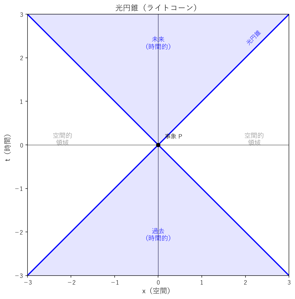
The line element of Minkowski spacetime is
We introduce Rindler coordinates \((\eta, \xi)\) defined by
(the \(y\) and \(z\) directions are left untransformed).
(a) Find the components of the Jacobian matrix: \(\dfrac{\partial(ct)}{\partial \eta}\), \(\dfrac{\partial(ct)}{\partial \xi}\), \(\dfrac{\partial x}{\partial \eta}\), \(\dfrac{\partial x}{\partial \xi}\).
(b) Using the transformation law for the metric tensor, show that the line element in Rindler coordinates is
(c) The metric tensor component \(g_{\eta\eta} = -\xi^2\) depends on \(\xi\). Discuss the physical meaning of this in relation to the equivalence principle argument from Ch. 5 — "in a uniform gravitational field, the rate at which time passes differs from place to place."
(a) Components of the Jacobian Matrix:
From \(ct = \xi\sinh\eta\), \(x = \xi\cosh\eta\):
(Rows correspond to \((ct, x)\), columns correspond to \((\eta, \xi)\))
(b) Derivation of the Line Element in Rindler Coordinates:
The Minkowski metric is \(g_{\mu\nu} = \text{diag}(-1, +1, +1, +1)\). Since the \(y\) and \(z\) directions are not transformed, we consider only the \((ct, x)\) part.
Applying the transformation rule \(g'_{kl} = \dfrac{\partial x^\mu}{\partial u^k}\dfrac{\partial x^\nu}{\partial u^l}\,g_{\mu\nu}\):
Calculation of \(g'_{\eta\eta}\):
Here we used the hyperbolic identity \(\cosh^2\eta - \sinh^2\eta = 1\).
Calculation of \(g'_{\xi\xi}\):
Calculation of \(g'_{\eta\xi}\):
Since the \(y\) and \(z\) directions are not transformed, \(g'_{yy} = 1\), \(g'_{zz} = 1\).
Therefore:
Verification: \(\det J = \xi\cosh^2\eta - \xi\sinh^2\eta = \xi\), so the transformation is non-singular for \(\xi > 0\). Also, the worldline with \(\xi = \text{const}\) satisfies \(x^2 - c^2t^2 = \xi^2\), which is a hyperbola corresponding to the worldline of uniformly accelerated motion. ✓
(c) Discussion of Physical Meaning:
Rindler coordinates describe the coordinate system of an observer undergoing uniform acceleration with magnitude \(a = c^2/\xi\). By the equivalence principle, this coordinate system is locally equivalent to a stationary coordinate system in a uniform gravitational field.
Physical meaning of \(g_{\eta\eta} = -\xi^2\) depending on \(\xi\):
The relationship between coordinate time \(\eta\) and proper time \(\tau\) for a stationary observer (\(d\xi = dy = dz = 0\)) is:
(In units where \(c = 1\): \(d\tau = \xi\,d\eta\))
This means that even when the same coordinate time \(d\eta\) elapses, proper time advances at different rates at locations with different values of \(\xi\). Specifically:
- At locations with large \(\xi\) ("upward" in the acceleration direction; in the gravitational analogy, where the gravitational potential is higher), proper time advances faster
- At locations with small \(\xi\) ("downward"; where the gravitational potential is lower), proper time advances slower
- As \(\xi \to 0\), \(g_{\eta\eta} \to 0\), and the advance of proper time stops (the Rindler horizon)
This is precisely the manifestation of gravitational time dilation discussed in Ch. 5. According to the equivalence principle, in a uniform gravitational field, "time passes faster at higher locations." The \(\xi\) dependence of \(g_{\eta\eta} = -\xi^2\) in the Rindler metric precisely expresses this effect in the language of the metric tensor.
Relation to gravitational redshift:
When two observers at different \(\xi\) positions exchange signals with the same coordinate time interval \(\Delta\eta\), their respective proper time intervals are \(\Delta\tau_1 = \xi_1\,\Delta\eta\) and \(\Delta\tau_2 = \xi_2\,\Delta\eta\). When \(\xi_1 < \xi_2\), we have \(\Delta\tau_1 < \Delta\tau_2\), meaning that light emitted from "below" appears redshifted to the observer "above." This is gravitational redshift, a direct consequence derived from the equivalence principle.
Supplementary note: \(\xi = 0\) is called the Rindler horizon, corresponding to the boundary that is causally inaccessible from the perspective of the uniformly accelerating observer. This shares similarities with the event horizon of a black hole and serves as an important model for understanding the physics of horizons in general relativity.
Feedback on this page
Let us know if something was unclear, incorrect, or could be improved.