Chapter 3: The Double-Slit Experiment — The Collapse of Determinism and Realism
Story so far:
In Ch. 1, we saw that three crises—black-body radiation, the photoelectric effect, and atomic stability—made the discreteness of energy (quantization) unavoidable. In Ch. 2, through de Broglie's matter wave hypothesis and electron diffraction experiments, we confirmed that particles also exhibit wave-like behavior. But what exactly does it mean for "a particle to behave like a wave"? What is "waving"? This chapter's experiment confronts that question head-on.
Goals of this chapter
We will follow the electron double-slit experiment (both as a thought experiment and an actual experiment) in detail, leading to three conclusions: 1. Individual electrons are detected as particles, but when many are collected, they produce an interference pattern 2. If you determine "which slit the electron passed through," the interference disappears 3. Neither the classical particle picture nor the wave picture can fully explain this phenomenon — probability plays an essential role, and determinism collapses
3.1 The Bullet Double-Slit — Baseline for Classical Particles
🟡 Lina: Today we'll take on the most famous experiment in quantum mechanics — the double-slit experiment. But rather than shooting electrons right away, let's first confirm what happens when we do the same experiment with everyday particles — bullets.
🔵 Kai: Bullets through a double slit? That sounds dangerous.
🟡 Lina: It's a thought experiment, so don't worry. Here's the setup:
- A machine gun sprays bullets in random directions
- In front of it is a wall with two slits (slit 1 and slit 2)
- Behind the wall is a backstop with a detector that can be moved along position \(x\)
For bullets, it's more natural to call them "holes," but since we'll compare with electron and wave experiments later, I'll use "slit" and "hole" interchangeably. Both just mean an opening in the wall.
🟡 Lina: We assume the bullets are idealized — they never break apart. They never split in half. When they reach the detector, they always arrive as one whole bullet. And since the wall has only two slits, each bullet must pass through one or the other. That is, "passes through slit 1" and "passes through slit 2" never happen simultaneously — they are mutually exclusive events in probability terms.
⚪ Mei: If they can't break and can't pass through the wall, then each bullet must go through either slit 1 or slit 2 — mutually exclusive events.
🟡 Lina: Exactly. We fire bullets for a sufficiently long time and measure the arrival probability \(P(x)\) at each detector position \(x\). Let's compare three cases:
- Slit 2 blocked: Bullets pass only through slit 1 → probability distribution \(P_1(x)\)
- Slit 1 blocked: Bullets pass only through slit 2 → probability distribution \(P_2(x)\)
- Both slits open: probability distribution \(P_{12}(x)\)
🔵 Kai: When both are open, shouldn't it just be \(P_1\) plus \(P_2\)? Since each bullet goes through one or the other.
🟡 Lina: Exactly right. The experimental result is:
⚪ Mei: "Passing through hole 1" and "passing through hole 2" are mutually exclusive events, so the total probability is the sum of the individual probabilities — just like the addition rule we learned in high school probability.
🟡 Lina: Right. We'll call this result "no interference." See Fig. 3.1 "Conceptual diagram of the bullet double-slit experiment" for an overview of the experiment. Why we call it "no interference" will become clear when we see the wave experiment next. The "interference fringes" we'll see in the next section never appear for bullets — that's what "no interference" means.
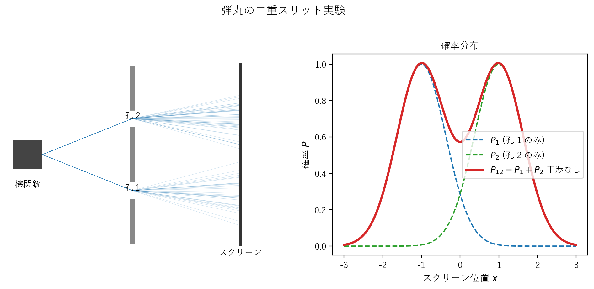
Fig. 3.1: Conceptual diagram of the bullet double-slit experiment. Bullets fired from the machine gun pass through one hole or the other, and the probability distribution follows \(P_{12} = P_1 + P_2\). The "interference fringes" seen in the next section do not appear.
✅ Comprehension Check: State the physical reason why \(P_{12} = P_1 + P_2\) holds in the bullet double-slit experiment.
Answer
Bullets are indestructible particles that must pass through either hole 1 or hole 2. "Passing through hole 1" and "passing through hole 2" are mutually exclusive events, so by the addition rule of probability, the total probability equals the sum of the individual probabilities.
3.2 The Water Wave Double-Slit — Mathematical Structure of Interference
🟡 Lina: Next, let's do the same experiment with water waves. We place a wave source in a shallow tank, generating circular waves. The wall has two slits, and behind it we place a detector. The detector measures the intensity of the wave. Intensity is a quantity representing the magnitude of the wave's energy — think of it as "the more vigorously the wave oscillates, the greater the intensity."
🔵 Kai: How exactly do you calculate intensity? It's different from the wave height itself, right?
🟡 Lina: Right. Let's write the water surface height (displacement) as \(h\). This is the same letter as Planck's constant, but in this section we're talking about water waves, so don't confuse them — distinguish by context. We used the same notation in the Prologue. Intensity is proportional to the square of the wave's amplitude (the maximum displacement) — why squared? Because the energy of a wave increases with larger oscillation amplitude, and physically it's proportional to the square of the amplitude. You can think of each point on the water surface as vibrating up and down like a spring, so just as a spring's elastic energy is proportional to the square of displacement \(\frac{1}{2}kx^2\), wave energy is also proportional to the square of amplitude.
🔵 Kai: I see, each point on the water oscillates like a spring, so energy is proportional to amplitude squared... that makes sense. But why are complex numbers about to appear?
🟡 Lina: Good question. To calculate interference, we'll represent \(h\) as a complex number. When written as a complex number, what corresponds to "amplitude" (the real maximum displacement) in high school physics is \(|h|\) (the absolute value of the complex number). So intensity is written as \(I \propto |h|^2\) — by taking the absolute value squared, we always get a real positive value. Let me explain the reason first: a wave carries two pieces of information — "amplitude (magnitude of oscillation)" and "phase (which stage of crest/trough it's in)." A single real number can only represent amplitude, but with a complex number we can write \(h = |h|e^{i\theta}\) and pack both amplitude \(|h|\) and phase \(\theta\) into a single number. And when we add two waves, the phase difference automatically produces the interference effect — you'll see this in the calculation coming up.
Let's look at a concrete example. Suppose there are two waves with amplitude 1, one at a crest (phase \(0\)) and the other at a trough (phase \(\pi\)). In real numbers: \(h_1 = 1\), \(h_2 = -1\), and adding them gives \(h_1 + h_2 = 0\) — they cancel. In complex numbers: \(h_1 = 1 \cdot e^{i \cdot 0} = 1\), \(h_2 = 1 \cdot e^{i\pi} = -1\) — same result. But what if the phase is some intermediate value like \(\pi/3\)? With real numbers alone, you can't represent "amplitude 1 at phase \(\pi/3\)" as a single number. With complex numbers, you can write \(h = e^{i\pi/3} = \cos(\pi/3) + i\sin(\pi/3)\), and just adding gives you the interference effect automatically.
⚪ Mei: So complex numbers let you pack "magnitude" and "timing" into a single number, and interference comes out automatically from addition — a convenient tool.
🟡 Lina: Exactly. To summarize: writing \(h = |h|e^{i\theta}\), \(|h|\) is the amplitude, \(\theta\) is the phase, and when adding two waves, the interference effect is automatically reflected. When calculating the observable physical quantity (intensity), we take \(|h|^2\), so the final result is always real.
Now let's examine the same three cases as with bullets:
- Hole 2 blocked: Intensity of wave spreading from hole 1 → \(I_1(x) = |h_1(x)|^2\)
- Hole 1 blocked: Intensity of wave spreading from hole 2 → \(I_2(x) = |h_2(x)|^2\)
- Both holes open: Intensity \(I_{12}(x) = ?\)
🔵 Kai: Since it's a wave, we can use the superposition principle. With both open, the wave height becomes \(h_1 + h_2\).
🟡 Lina: Correct. Now calculate the intensity.
⚪ Mei: Intensity is the absolute value squared of the amplitude, so \(I_{12} = |h_1 + h_2|^2\).
🟡 Lina: Right. Let's expand this. We'll use the formula for expanding the absolute value squared of a complex number. We write \(h_1\) and \(h_2\) in polar form. Polar form means representing a complex number as "magnitude × rotation" — writing \(h = |h|e^{i\theta}\), where \(|h|\) is the amplitude magnitude and \(e^{i\theta} = \cos\theta + i\sin\theta\) (Euler's formula) represents the phase rotation. This is the same notation as when we wrote the de Broglie wave as \(e^{i(kx - \omega t)}\) in Ch. 2. You've probably written complex numbers as \(r(\cos\theta + i\sin\theta)\) in high school. Using Euler's formula \(e^{i\theta} = \cos\theta + i\sin\theta\), you can abbreviate this as \(re^{i\theta}\) — the relationship introduced in Ch. 2. What matters for our calculation is just the correspondence "\(e^{i\theta}\) means \(\cos\theta + i\sin\theta\)" — just remember that and you'll be fine. Writing \(h_1 = |h_1|e^{i\theta_1}\), \(h_2 = |h_2|e^{i\theta_2}\), the angles \(\theta_1\), \(\theta_2\) are the phases of each wave when they arrive at detector position \(x\) — the angle representing which stage of "crest" and "trough" the wave is in.
🔵 Kai: I'm fine with polar form from the previous chapter. So we want to expand \(|h_1 + h_2|^2\). Can we just expand it like \((h_1 + h_2)^2\)?
🟡 Lina: Close, but not quite. Since it's the absolute value squared, it's slightly different from just squaring. To expand \(|h_1 + h_2|^2\), it's convenient to rewrite the absolute value squared as a "product form" — because then we can use the distributive law (expanding brackets). The tool for this is the complex conjugate.
Before that, one notational convention. In the Prologue we wrote the complex conjugate as \(\bar{z}\), but in physics the standard notation is \(z^*\). We'll use this notation from now on. The meaning is exactly the same — just flip the sign of the imaginary part.
For a complex number \(h\), flipping the sign of the imaginary part gives the complex conjugate, written \(h^*\). For example, if \(h = 3 + 2i\) then \(h^* = 3 - 2i\). And \(|h|^2 = h^* h\) holds. Let's verify: \(h^* h = (3 - 2i)(3 + 2i) = 9 + 4 = 13\), which matches \(3^2 + 2^2 = 13\). In general, if \(h = a + bi\) then \(h^* h = (a - bi)(a + bi) = a^2 + b^2 = |h|^2\).
⚪ Mei: So by rewriting the absolute value squared as the product \(z^* z\), we can use the distributive law.
🟡 Lina: Right. Let's use this to expand \(|h_1 + h_2|^2\). Using \(|z|^2 = z^* z\) with \(z = h_1 + h_2\), we get \(|h_1 + h_2|^2 = (h_1 + h_2)^*(h_1 + h_2)\). Next, the complex conjugate of a sum is the sum of the complex conjugates — that is, \((h_1 + h_2)^* = h_1^* + h_2^*\). This can be verified from the definition: if \(h_1 = a + bi\), \(h_2 = c + di\), then \(h_1 + h_2 = (a+c) + (b+d)i\), and its complex conjugate is \((a+c) - (b+d)i = (a - bi) + (c - di) = h_1^* + h_2^*\).
Using this:
🔵 Kai: The first two terms \(|h_1|^2 + |h_2|^2\) are just the intensities of each wave alone. The last two terms \(h_1^* h_2 + h_2^* h_1\) are the "extra" part that appeared... is that the interference term?
🟡 Lina: Yes, that's exactly the interference term. Let's compute the last two terms explicitly. Remember we wrote \(h = |h|e^{i\theta}\) — this "magnitude × rotation" form is called polar form. Let's substitute. First, a check — what's the complex conjugate of polar form \(h = |h|e^{i\theta}\)? Since \(e^{i\theta} = \cos\theta + i\sin\theta\), flipping the sign of the imaginary part gives \(\cos\theta - i\sin\theta = e^{-i\theta}\). So \(h^* = |h|e^{-i\theta}\) — just the sign in the exponent flips. Using this:
Similarly \(h_2^* h_1 = |h_1||h_2|e^{i(\theta_1 - \theta_2)}\). Adding these two, using the relation \(e^{i\alpha} + e^{-i\alpha} = (\cos\alpha + i\sin\alpha) + (\cos\alpha - i\sin\alpha) = 2\cos\alpha\):
⚪ Mei: The \(e^{i\alpha} + e^{-i\alpha} = 2\cos\alpha\) makes the imaginary parts cancel, so the interference term is real.
🟡 Lina: Right. Since the physical intensity is real, any term added to it must also be real — and it all checks out. Here \(\delta = \theta_2 - \theta_1\) is called the phase difference between the two waves. Since \(\cos\) is an even function, \(\cos(\theta_2 - \theta_1) = \cos(\theta_1 - \theta_2)\), so the sign convention doesn't matter. The phase difference \(\delta\) varies with position because the distance from hole 1 to the detector differs from the distance from hole 2 to the detector at each location — the phase difference is determined by how many wavelengths fit in the path length difference. So as you move the detector, \(\delta\) changes continuously, \(\cos\delta\) oscillates between \(+1\) and \(-1\), and a pattern of bright and dark fringes emerges.
Since we defined \(I_1 = |h_1|^2\), \(I_2 = |h_2|^2\) earlier, we have \(|h_1| = \sqrt{I_1}\), \(|h_2| = \sqrt{I_2}\) (amplitudes are non-negative, so we take the positive square root). Therefore \(|h_1||h_2| = \sqrt{I_1 I_2}\), and:
🔵 Kai: Oh, there's an extra term added to \(I_1 + I_2\)!
🟡 Lina: This extra term \(2\sqrt{I_1 I_2}\cos\delta\) is called the interference term.
⚪ Mei: Depending on the value of \(\cos\delta\), it can be constructive (\(\cos\delta = +1\)) or destructive (\(\cos\delta = -1\)). Since the phase difference \(\delta\) varies with position, a pattern of bright and dark fringes appears.
🟡 Lina: Yes. This is the interference pattern. It's clearly different from the bullet result, equation (3.1).
🔵 Kai: Bullets add probabilities, waves add amplitudes. The results are completely different.
🟡 Lina: Look at Fig. 3.2 "Water wave double-slit experiment". Comparing the intensity distributions with only hole 1 open, only hole 2 open, and both open, you can clearly see that with both open, a pattern completely different from \(I_1 + I_2\) appears.
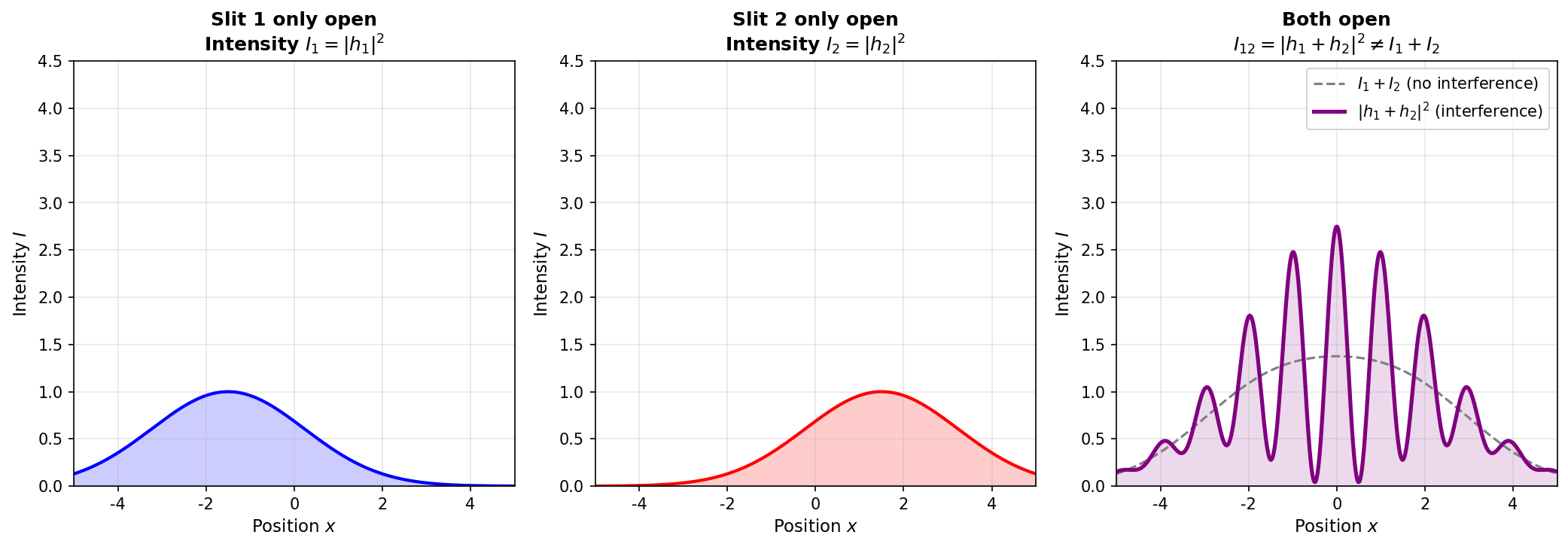
Fig. 3.2: Water wave double-slit experiment. Left: Intensity \(I_1\) with only hole 1 open. Center: Intensity \(I_2\) with only hole 2 open. Right: Intensity \(I_{12} = |h_1 + h_2|^2\) with both open (solid line) differs from \(I_1 + I_2\) (dashed line), showing bright and dark fringes due to interference.
🟡 Lina: That's exactly the key point. For waves, you add amplitudes first, then square. For particles, you add probabilities (which are already squared). This difference generates the interference term.
✅ Comprehension Check: In equation (3.2), when \(\delta = \pi\) (phase difference of half a wavelength) and \(I_1 = I_2 = I_0\), what is \(I_{12}\)?
Answer
Since \(\cos\pi = -1\), we get \(I_{12} = I_0 + I_0 + 2\sqrt{I_0 \cdot I_0}(-1) = 2I_0 - 2I_0 = 0\). Complete destructive interference — the intensity becomes zero.
📝 Exercises:
- Derivation of double-slit interference conditions → Problem M-4. Understanding the Disappearance of Interference through "Conditional Decomposition of Probability"
3.3 The Electron Double-Slit — Particles That Interfere
🟡 Lina: Now for the main event. What happens when we do the same double-slit experiment with electrons?
🔵 Kai: Since we learned in Ch. 2 that electrons have wave properties... they should interfere, right?
🟡 Lina: Don't rush to the conclusion. Let's first confirm the experimental setup.
- Electron gun: Electrons are emitted from a heated filament and accelerated by a voltage. This produces an electron beam with nearly uniform energy
- Wall with two slits: Two microscopic slits are cut in a thin metal plate
- Detector: Placed on a screen. When an electron arrives, it produces a "click" signal
🔵 Kai: Does the detector count them one by one, like with bullets?
🟡 Lina: Yes. And this is a crucially important fact. Let me state the first key feature of the experimental results.
Fact 1: Electrons are detected as particles
🟡 Lina: Moving the detector and recording electron arrivals, we find:
- The detector produces discrete "clicks"
- The clicks arrive at irregular intervals
- But each click has the same magnitude — "half an electron" is never detected
⚪ Mei: Just like bullets. Electrons arrive at the detector one whole particle at a time. They don't spread out continuously like a wave.
🟡 Lina: Right. Electrons are detected as particles. So far, same as bullets.
Fact 2: Collecting many electrons reveals an interference pattern
🟡 Lina: However, when we detect electrons over a long period and determine the arrival probability \(P_{12}(x)\) at each position \(x\) —
🔵 Kai: Don't tell me...
🟡 Lina: Yes. The same pattern as water wave interference appears.
Near the center, there are places where \(P_{12}\) exceeds \(P_1 + P_2\) by more than a factor of two, and places where it's nearly zero. Bright and dark fringes — an interference pattern.
🔵 Kai: Wait a moment. Electrons arrive one at a time as particles with a "click," right? Yet the overall pattern is the same as wave interference? And there are places where it's more than twice \(P_1 + P_2\) — that would be absolutely impossible for bullets — having a higher probability than with one hole blocked.
🟡 Lina: Exactly. This is the central mystery of quantum mechanics. Look at Fig. 3.3 "Conceptual diagram of the electron double-slit experiment. Electrons fired from the electron gun are detected one at a time as particles, yet the accumulated probability distribution \(P_{12}\) is completely different from \(P_1 + P_2\)" while I say this once more clearly:
Electrons are detected one at a time as particles. Yet the probability distribution of many electrons has the same shape as a wave interference pattern.
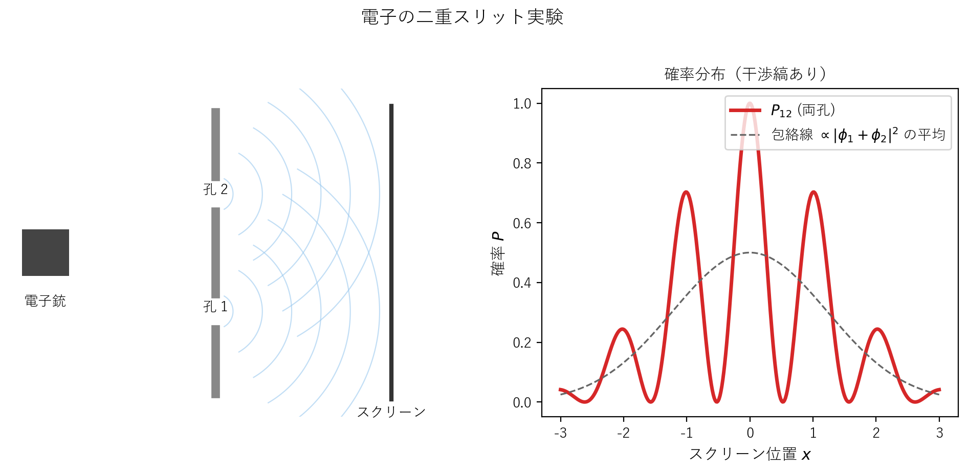
Fig. 3.3: Conceptual diagram of the electron double-slit experiment. Electrons fired from the electron gun are detected one at a time as particles, yet the accumulated probability distribution \(P_{12}\) is completely different from \(P_1 + P_2\) — it shows a wave interference pattern.
🔵 Kai: But couldn't this just be because many electrons are flying simultaneously and interfering with each other through collisions?
🟡 Lina: Good question, but no. In fact, even when electrons are fired one at a time — meaning the next electron is launched only after the previous one has been detected — if you collect enough of them, the same interference pattern appears. This was beautifully demonstrated in 1989 by Akira Tonomura and colleagues. When electrons are sent one at a time, initially only random dots scatter across the screen. But as thousands, then tens of thousands accumulate, the interference pattern gradually emerges.
🔵 Kai: A single electron... interfering with itself?
🟡 Lina: In classical language, that's how you'd want to describe it. But more precisely, it's that "classical language" itself cannot be applied. We'll discuss this more shortly. Look at Fig. 3.4 "Emergence of interference fringes through electron accumulation". With only about 10 electrons, it looks like nothing but random dots, but once 10,000 have accumulated, the interference fringes clearly emerge.
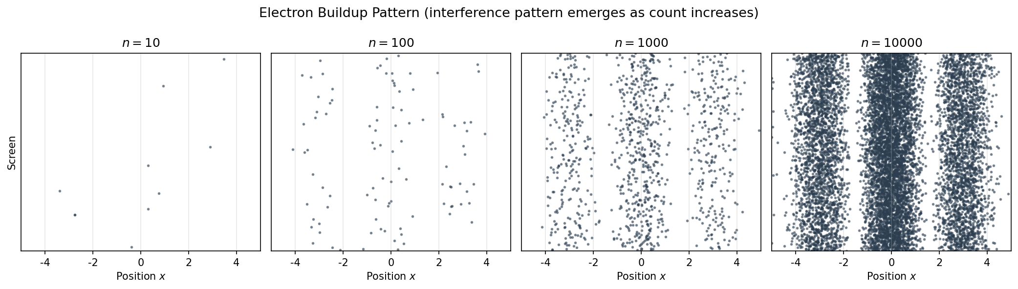
Fig. 3.4: Emergence of interference fringes through electron accumulation. The accumulation pattern on the screen when electrons are sent one at a time. With few electrons (\(n=10\)), just random dots appear, but with many (\(n=10000\)), interference fringes emerge. In classical language, it appears as if "a single electron interferes with itself," but precisely this expression reveals the limits of the classical framework.
Mathematical description of the interference pattern
🟡 Lina: When we had water waves, intensity was calculated by "adding amplitudes then squaring." It turns out the same mathematical structure describes the electron case. Let me formally use the probability amplitude previewed in the Prologue. We define two complex numbers \(\phi_1(x)\) and \(\phi_2(x)\):
- Only hole 1 open: \(P_1 = |\phi_1|^2\)
- Only hole 2 open: \(P_2 = |\phi_2|^2\)
- Both open: \(P_{12} = |\phi_1 + \phi_2|^2\)
Here \(\mathrm{Re}(z)\) is the operation of taking the real part of a complex number \(z\) — if \(z = a + bi\) then \(\mathrm{Re}(z) = a\). Why this notation? Because \(\phi_1^* \phi_2\) is generally complex, but only its real part has physical significance as an interference term. Using the same calculation as for water waves, \(\phi_1^* \phi_2 = |\phi_1||\phi_2|e^{i(\theta_2 - \theta_1)}\), so \(2\mathrm{Re}(\phi_1^* \phi_2) = 2|\phi_1||\phi_2|\cos\delta\). That is, the interference term \(2\sqrt{I_1 I_2}\cos\delta\) from equation (3.2) for water waves can also be written as \(2\mathrm{Re}(h_1^* h_2)\) — just a different notation for the same thing. The \(\mathrm{Re}\) notation is convenient because it shows the structure of the interference term without expanding into polar form — we'll use it frequently from now on. For electrons, it's exactly the same mathematical structure with \(h\) replaced by \(\phi\).
🔵 Kai: This has exactly the same structure as equation (3.2) for water waves! But what are \(\phi_1\) and \(\phi_2\)? For water waves it was "wave height," but for electrons...?
🟡 Lina: Good question. \(\phi_1\) and \(\phi_2\) are complex numbers called probability amplitudes. They are not directly observable physical quantities like the "height" of a water wave. What can be observed is only \(|\phi|^2\), the probability.
✅ Comprehension Check: What is a probability amplitude? And what is the crucial difference between the "amplitude" of a water wave and the "probability amplitude" of an electron?
Answer
A probability amplitude is a complex number whose absolute value squared gives a probability. The amplitude of a water wave (wave height) is a directly observable physical quantity, but an electron's probability amplitude cannot be directly observed — only \(|\phi|^2\) (probability) is observable.
⚪ Mei: So for electrons, instead of "adding probabilities," we "add probability amplitudes" and then square — that's the point.
🟡 Lina: Exactly. This is the fundamental difference between classical probability calculation and quantum mechanical probability calculation. I've compiled the three cases in a table, so look at Table 3.1 "Probability composition rules for bullets, water waves, and electrons" to organize your thinking. The probability distributions for all three cases are also plotted side by side in Fig. 3.5 "Probability distribution comparison for bullets, waves, and electrons", so compare them.
Table 3.1: Probability composition rules for bullets, water waves, and electrons
| Classical particle (bullet) | Wave (water wave) | Electron | |
|---|---|---|---|
| What you add | Probabilities | Amplitudes | Probability amplitudes |
| How detected | As particles | Continuously | As particles |
| Interference | None | Yes | Yes |
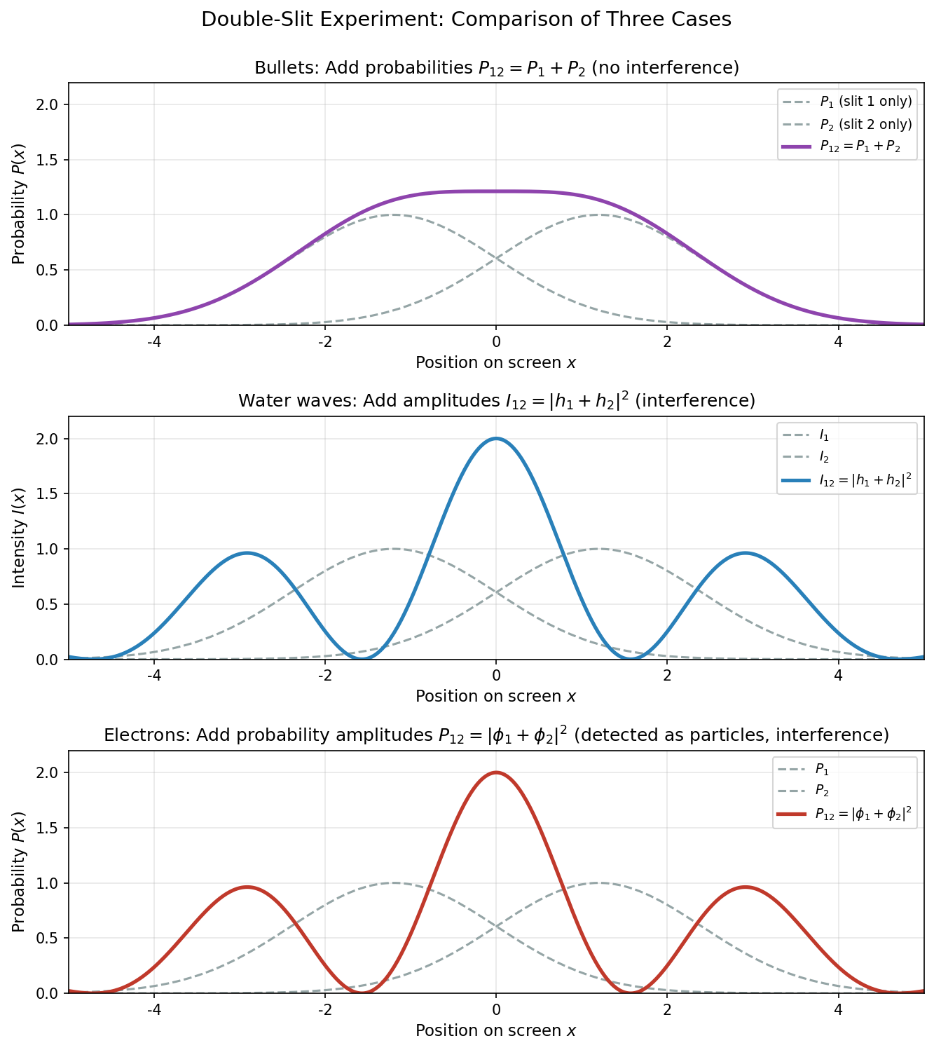
Fig. 3.5: Probability distribution comparison for bullets, waves, and electrons. The probability distributions on the screen for the three cases. Bullets give \(P_{12} = P_1 + P_2\) (simple addition), while water waves and electrons show interference fringes because amplitudes are added before squaring. Electrons and water waves have mathematically identical interference patterns, but the crucial difference is that electrons are detected as particles.
🔵 Kai: Electrons are "detected as particles" yet "we add amplitudes"... isn't that contradictory? If they're "particles" we should add probabilities, and if they're "waves" we should add amplitudes but they should arrive continuously. It's neither?
🟡 Lina: Right, it's neither. Look again at Table 3.1 "Probability composition rules for bullets, water waves, and electrons" and Fig. 3.5 "Probability distribution comparison for bullets, waves, and electrons" — the differences among the three cases of bullets, waves, and electrons are immediately clear. If you try to force electrons into the classical categories of "particle" or "wave," you get contradictions. The quantum mechanical approach doesn't try to resolve this "contradiction" but rather accepts the experimental facts as they are and formulates them mathematically. We give up trying to define "what an electron is" in classical terms, and instead describe "what an electron does" using the rules of probability amplitudes. At the end of this section, we'll look more closely at why the classical picture breaks down.
✅ Comprehension Check: In the electron double-slit experiment, name one thing in common with the bullet experiment and one difference.
Answer
In common: Electrons are detected discretely one at a time (as particles). "Half an electron" does not exist. Different: The probability distribution of many electrons does not satisfy \(P_{12} = P_1 + P_2\) and shows an interference pattern.
📝 Exercises:
- Sign of interference term and bright/dark fringes → Problem B-1. Calculation of Interference Terms
3.4 Asking "Which One Did It Pass Through?" — Observation and the Disappearance of Interference
🔵 Kai: I've been wondering about this for a while — why not just look to see which hole the electron went through? Shine light on it.
🟡 Lina: Let's do exactly that experiment. We place a strong light source just behind the wall to illuminate electrons passing near the holes. If an electron scatters a photon, we'll see a flash of light. The position of the flash tells us whether the electron passed through hole 1 or hole 2.
Experimental result: when you can tell which way it went
🟡 Lina: When we turn on the light source and run the experiment, here's what happens:
- Each time an electron arrives at the detector with a "click," a flash of light is seen near either hole 1 or hole 2
- The flash always occurs at one or the other — it never lights up at both simultaneously
🔵 Kai: Yes! So the electron really does pass through one or the other!
🟡 Lina: ...That's what you'd think, right? But here's the problem. With the light source on, we sort the electrons: collect those confirmed to have "passed through hole 1" and build probability distribution \(P_1'(x)\), collect those confirmed to have "passed through hole 2" and build \(P_2'(x)\). Then —
And the overall probability distribution is:
⚪ Mei: ...The interference fringes have disappeared!
🟡 Lina: Yes. When you determine "which way it went," the interference vanishes. Looking at Fig. 3.6 "Disappearance of interference fringes due to observation. The difference in probability distributions with and without observation. Left: When "which slit it passed through" is not observed, interference fringes appear. Right: When observed, the contributions from each slit simply add up, and interference fringes disappear. Observation changes the result itself", you can see at a glance how the distribution changes with and without observation.
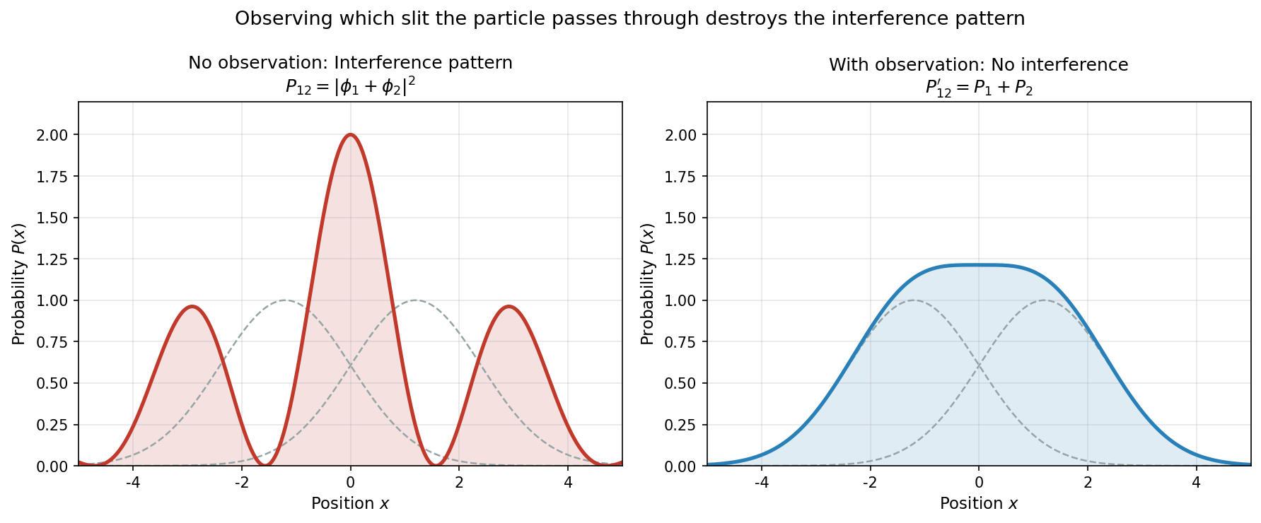
Fig. 3.6: Disappearance of interference fringes due to observation. The difference in probability distributions with and without observation. Left: When "which slit it passed through" is not observed, interference fringes appear. Right: When observed, the contributions from each slit simply add up, and interference fringes disappear. Observation changes the result itself — a core property of quantum mechanics.
✅ Comprehension Check: When you observe which slit the electron passed through using light, how does the probability distribution change?
Answer
The interference fringes disappear, and the probability distribution becomes \(P_{12}' = P_1 + P_2\). That is, it returns to the same simple addition as for classical particles (bullets). When information about "which way it went" is obtained, the interference term vanishes.
🔵 Kai: Huh... it interferes when you don't shine light on it, but stops interfering when you do? Is the light disturbing the electron?
🟡 Lina: That's the natural thought. Indeed, a photon imparts momentum to the electron and disturbs its trajectory — this is a fact. As we saw with Compton scattering in Ch. 2, the momentum per photon is \(p = h/\lambda\) (\(h\) is Planck's constant), so the longer the wavelength, the smaller the momentum. So maybe we can reduce the disturbance by using longer wavelength light? ...But when you try, things aren't so simple.
The longer-wavelength experiment
🟡 Lina: As you gradually increase the wavelength of light, two things happen simultaneously:
- The disturbance to the electron decreases → the interference pattern begins to recover
- However, as wavelength increases, the resolution of the light drops → you can no longer distinguish which hole the electron passed through
"Resolution drops" means the following. If the spacing between the two slits is \(d\), then to distinguish "was the electron near hole 1 or hole 2," you need to localize its position to at least precision \(d\). However, light has a fundamental limit: "it cannot distinguish positions finer than its wavelength." A wave cannot "see" structures narrower than its own wavelength — for example, if you throw a stone into a pond, a wave with wavelength 1 m barely notices a 10 cm post and simply diffracts around it. This is the same principle you learned in high school physics: "when the slit width is comparable to the wavelength, diffraction occurs and light spreads out."
🔵 Kai: Ah, we covered that with diffraction. When a wave passes through a gap narrower than its wavelength, it spreads out and you lose directional information.
🟡 Lina: Right. When a photon is scattered by something, the scattered photon itself spreads as a wave. The width of that spread is on the order of the wavelength \(\lambda\) — meaning the photon cannot carry information about "where within a region narrower than its own wavelength it was scattered." This is also the flip side of de Broglie's relation \(\lambda = h/p\) from Ch. 2 — to know position to precision \(\Delta x\), you need light with wavelength \(\lambda \lesssim \Delta x\). Such a photon has momentum \(p = h/\lambda \gtrsim h/\Delta x\), so the more precisely you try to know the position, the larger the photon momentum needed, and the greater the disturbance to the electron.
⚪ Mei: Trying to know position precisely increases the momentum disturbance, and trying to reduce disturbance makes position unknowable — it's a trade-off.
🟡 Lina: Exactly. Intuitively, it's like trying to find a small button while wearing thick gloves. Short wavelength means "thin fingers" that can feel the position, but long wavelength means "thick fingers" that can't distinguish. So when the light wavelength \(\lambda\) exceeds the slit spacing \(d\) (\(\lambda > d\)), you can no longer tell near which slit the photon was scattered.
🔵 Kai: So... when interference fringes are visible, you can't tell "which way it went," and when you can tell "which way it went," the interference fringes disappear?
🟡 Lina: Precisely. This isn't a matter of "maybe with a cleverer method you could see both simultaneously." No matter what experimental method you try, the following conclusion remains unchanged:
Whenever it is in principle possible to identify which slit the electron passed through, the interference pattern disappears. Only when identification is in principle impossible does the interference pattern appear.
🔵 Kai: "In principle" — does that mean even if you don't actually look?
🟡 Lina: Yes. Even if you don't actually check which detector the photon entered, the mere possibility of checking causes the interference to disappear. In other words, it's determined by whether the distinguishing information exists anywhere in the universe. Whether you actually read it out is irrelevant.
⚪ Mei: What matters isn't "whether you looked" but "whether the information exists."
Mathematical organization: distinguishability and how to add probabilities
🟡 Lina: Let me organize the mechanism by which interference disappears mathematically. In the experiment with the light source, we need to consider the "total system" including not just the electron but also the photon's state.
There are two variables to consider: "which hole the electron passed through" (hole 1 or hole 2) and "which detector the scattered photon goes to" (\(D_1\) or \(D_2\)). Two choices × two choices gives four combinations total. We define one amplitude for each combination.
We place photon detectors \(D_1\) (near hole 1) and \(D_2\) (near hole 2). I'll define four complex amplitudes (the absolute value squared of each gives the probability that, "given the electron passed through that hole," the photon goes to that detector):
Amplitudes for photon detected at \(D_1\):
- \(a\): electron passed through hole 1 → photon goes to nearby \(D_1\) ("correct")
- \(b\): electron passed through hole 2 → photon goes to distant \(D_1\) ("wrong")
Amplitudes for photon detected at \(D_2\):
- \(b'\): electron passed through hole 1 → photon goes to distant \(D_2\) ("wrong")
- \(a'\): electron passed through hole 2 → photon goes to nearby \(D_2\) ("correct")
A mnemonic: the \(a\)-type (\(a\), \(a'\)) are amplitudes for "photon goes to the detector near the hole the electron passed through" (correct), and \(b\)-type (\(b\), \(b'\)) are amplitudes for "photon goes to the far detector" (wrong). Unprimed (\(a\), \(b\)) are for the photon going to \(D_1\), primed (\(a'\), \(b'\)) are for the photon going to \(D_2\). So \(|a|^2\) means "given the electron passed through hole 1, the probability that the scattered photon reaches the nearby detector \(D_1\)."
Since the photon must enter either \(D_1\) or \(D_2\), if the electron passed through hole 1: \(|a|^2 + |b'|^2 = 1\), and if it passed through hole 2: \(|a'|^2 + |b|^2 = 1\). So \(|a|^2\) is "the probability that a photon from an electron that passed through hole 1 correctly goes to \(D_1\)."
🔵 Kai: Why is \(|a|^2 + |b'|^2 = 1\)?
🟡 Lina: The photon must go to either \(D_1\) or \(D_2\) — there's nowhere else for it to go. So "probability of going to \(D_1\)" + "probability of going to \(D_2\)" = 1. Since probability is the absolute value squared of the amplitude, \(|a|^2 + |b'|^2 = 1\). It's the same as learning in high school probability that "the sum of probabilities of all outcomes equals 1."
🔵 Kai: Oh, I see. It's just the fact that total probability is 1, written in terms of amplitudes. ...Also, I'm a bit confused by the distinction between \(a\) and \(a'\), \(b\) and \(b'\)...
🟡 Lina: Good point. Remember it this way: \(a\) and \(a'\) are amplitudes for "photon goes to the correct (nearby) detector" — \(a\) is electron through hole 1 → \(D_1\), \(a'\) is electron through hole 2 → \(D_2\). \(b\) and \(b'\) are amplitudes for "photon goes to the wrong (far) detector" — \(b\) is electron through hole 2 → \(D_1\), \(b'\) is electron through hole 1 → \(D_2\). So the \(a\)-type means "correct," the \(b\)-type means "wrong." And unprimed (\(a\), \(b\)) is the amplitude for the photon going to \(D_1\), primed (\(a'\), \(b'\)) is for going to \(D_2\) — organizing it this way makes the structure of equations (3.7) and (3.8) easier to see.
When the wavelength is short, \(a\) and \(a'\) are large while \(b\) and \(b'\) are small (a photon from an electron that passed through hole 1 preferentially goes to \(D_1\), and one from hole 2 goes to \(D_2\)). Conversely, when the wavelength is long, the photon can't distinguish which detector to go to, so \(a \approx b\) and \(a' \approx b'\).
Using these, the amplitude for "electron passes through hole 1, photon detected at \(D_1\)" is \(a\phi_1\), and "electron passes through hole 2, photon detected at \(D_1\)" is \(b\phi_2\). More carefully: \(\phi_1\) is the amplitude for "electron passes through hole 1 and arrives at position \(x\)," and \(a\) is the amplitude for "photon scattered near hole 1 reaches \(D_1\)." These two happen in succession, so the total amplitude is their product \(a\phi_1\). In high school probability, you learned "the probability that independent events A and B both occur is \(P(A) \times P(B)\)." The same idea applies here, but with amplitudes instead of probabilities: "the amplitude for successive processes is the product." This will be formally stated as Feynman's fundamental rule in the next chapter (Ch. 4). You can verify that ultimately \(|a\phi_1|^2 = |a|^2|\phi_1|^2\), which matches the product of probabilities, confirming it's a natural extension of the conventional rule.
🔵 Kai: So you're replacing the probability product rule with an amplitude product rule. Then how does equation (3.7) come about?
🟡 Lina: We want to find the probability of "electron at \(x\) and photon at \(D_1\)." There are two paths to this final state: "electron passes through hole 1, photon goes to \(D_1\)" (amplitude \(a\phi_1\)) and "electron passes through hole 2, photon goes to \(D_1\)" (amplitude \(b\phi_2\)). The crucial point is that the only information available at the end is "electron is at \(x\)" and "photon is at \(D_1\)." From the fact that the photon is at \(D_1\) alone, you cannot tell whether the electron went through hole 1 or hole 2 — if \(b \neq 0\), the photon can reach \(D_1\) via the hole-2 path too. Therefore, these two paths are indistinguishable, and we add amplitudes before squaring:
Similarly, the probability for "electron at \(x\) and photon at \(D_2\)" is:
🔵 Kai: Wait. I understand that for probabilities, "independent events multiply." But is it okay to multiply amplitudes the same way? Amplitudes aren't probabilities, right?
🟡 Lina: Good question. There are two key points.
First, the rule for probabilities was "probability of A followed by B = P(A) × P(B)." Since quantum mechanics uses amplitudes instead of probabilities, extending to "amplitude of A followed by B = (amplitude of A) × (amplitude of B)" is natural, right?
Second, this extension doesn't contradict the conventional rule. Why? Because the absolute value of a product of complex numbers equals the product of absolute values — \(|zw| = |z||w|\) — so \(|a\phi_1|^2 = |a|^2|\phi_1|^2\), which has the same form as the product of probabilities. (You can verify: \(|zw|^2 = (zw)^*(zw) = z^* w^* z w = |z|^2|w|^2\).)
So at the probability level it's consistent with conventional rules, and the results computed with this rule match experiments — that's the justification. In the next chapter we'll formalize this as Feynman's fundamental rule, but for now accept it as "the probability product rule translated to amplitudes."
🔵 Kai: Replacing the probability product with an amplitude product... the same idea as replacing probability addition with amplitude addition. So how do we use equations (3.7) and (3.8)?
🟡 Lina: Here's the crux. Equation (3.7) is the probability "given the photon is at \(D_1\)," and equation (3.8) is the probability "given the photon is at \(D_2\)." These two cases are distinguishable final states — by looking at the photon counter, you can tell whether it entered \(D_1\) or \(D_2\).
The quantum mechanical rule is:
For distinguishable final states, add probabilities (absolute values squared of amplitudes). Do not add amplitudes.
🔵 Kai: Wait. Earlier you said "for indistinguishable paths, add amplitudes." Why do we now add probabilities when they're distinguishable? Isn't adding amplitudes the default?
🟡 Lina: Good question. Think of it this way. When you add amplitudes, an interference term appears — meaning the two paths "mix together." But the situation where the photon is at \(D_1\) and the situation where it's at \(D_2\) are physically completely different situations. Concretely, after the experiment is over, looking at the photon detectors will always tell you "\(D_1\) clicked" or "\(D_2\) clicked." And a single photon never enters both \(D_1\) and \(D_2\) simultaneously — these two events never happen at the same time. It's exactly the structure of "mutually exclusive events have additive probabilities" from high school probability. Since mutually exclusive events A and B can't happen simultaneously, \(P(A \cup B) = P(A) + P(B)\). Distinguishable final states work the same way: "photon at \(D_1\)" and "photon at \(D_2\)" can't both be true simultaneously, so we add probabilities.
⚪ Mei: Mutually exclusive events mean you add probabilities — the same structure as the addition rule from high school appears in quantum mechanics as "distinguishable final states."
🟡 Lina: Right. Conversely, if we were to add amplitudes, it would mean "the world where the photon is at \(D_1\)" and "the world where the photon is at \(D_2\)" interfere with each other — but since looking at the detector confirms one or the other, such mixing can't occur. More concretely, interference happens when "two possibilities are indistinguishable, so you can't decide which was realized." But the moment the photon counter clicks and "\(D_1\)" is established, the other possibility is confirmed not to have been realized — so there's no room for mixing. This is less of an ultimate explanation of "why it works this way" and more a rule that should be accepted because it correctly reproduces experimental facts. When we organize this as Feynman's fundamental rules in the next chapter, we'll state it in a cleaner form.
🔵 Kai: I see... only when things are "indistinguishable" do amplitudes mix and produce interference.
🟡 Lina: Right. Now, what we want to know is "the probability that the electron arrives at position \(x\)." But in the experiment with the light source, every time an electron arrives, a photon also necessarily enters some detector. The case where the photon enters \(D_1\) and the case where it enters \(D_2\) are mutually exclusive — they can't happen simultaneously. So the total probability is the sum of the probabilities for these two cases.
🔵 Kai: Using the rule from before: "photon at \(D_1\)" and "photon at \(D_2\)" are distinguishable final states, so we add their respective probabilities — is that right?
🟡 Lina: Exactly. Equation (3.7) is "the probability when the photon is at \(D_1\)," equation (3.8) is "the probability when the photon is at \(D_2\)," so the total is:
🟡 Lina: In equation (3.5), we added \(\phi_1\) and \(\phi_2\) all together and then squared — meaning the amplitudes via hole 1 and via hole 2 mixed together, producing an interference term. On the other hand, in equation (3.9), we separate into two distinguishable cases — "photon at \(D_1\)" and "photon at \(D_2\)" — add amplitudes and square within each case, then add the resulting probabilities. Since amplitudes don't mix between cases, the interference between \(\phi_1\) and \(\phi_2\) is suppressed. The structure is: "compute probability for each distinguishable case and add them," while "within each case, add amplitudes of indistinguishable paths and then square" — a two-tier approach.
⚪ Mei: "Adding probabilities for each distinguishable case" is the same idea as the addition rule for mutually exclusive events in high school probability.
🟡 Lina: If the photon wavelength is short enough for perfect identification, \(b \approx 0\) and \(b' \approx 0\). Substituting \(b \approx 0\) into the first term of equation (3.9): \(|a\phi_1 + 0|^2 = |a\phi_1|^2\). Since the absolute value of a product of complex numbers equals the product of absolute values — \(|a\phi_1| = |a| \cdot |\phi_1|\) — we get \(|a\phi_1|^2 = |a|^2|\phi_1|^2\). Similarly the second term gives \(|a'\phi_2|^2 = |a'|^2|\phi_2|^2\). Therefore:
🔵 Kai: The interference term containing \(\phi_1^* \phi_2\) has completely vanished!
🟡 Lina: The interference term with \(\phi_1^* \phi_2\) disappears, leaving a weighted sum of \(P_1\) and \(P_2\) — the same "no interference" structure as bullets. Moreover, if \(b' \approx 0\) then \(|a|^2 \approx 1\) (since \(|a|^2 + |b'|^2 = 1\)), and similarly \(|a'|^2 \approx 1\), so \(P_{12}' \approx P_1 + P_2\), matching equation (3.6).
⚪ Mei: \(b \approx 0\) means "the probability that a photon from an electron that went through hole 1 ends up at \(D_2\) is nearly zero" — meaning the photon's destination completely reveals the path, so the interference term vanishes.
🟡 Lina: Exactly. Conversely, if the wavelength is so long that identification is impossible — since the photon wavelength exceeds the slit spacing, the photon can't carry information about "which hole it was scattered near." Whether the electron went through hole 1 or hole 2, the amplitude for the photon going to \(D_1\) becomes the same. So \(a = b\) and \(a' = b'\) (if the apparatus is symmetric, \(a = a'\) and \(b = b'\) also hold, but here \(a = b\) and \(a' = b'\) suffice). Substituting \(b = a\) into the first term of equation (3.9): \(|a\phi_1 + a\phi_2|^2 = |a(\phi_1 + \phi_2)|^2 = |a|^2|\phi_1 + \phi_2|^2\). Substituting \(b' = a'\) into the second term: \(|a'\phi_1 + a'\phi_2|^2 = |a'|^2|\phi_1 + \phi_2|^2\). Together: \((|a|^2 + |a'|^2)|\phi_1 + \phi_2|^2\). Substituting \(b' = a'\) into \(|a|^2 + |b'|^2 = 1\) gives \(|a|^2 + |a'|^2 = 1\), so the total equals \(|\phi_1 + \phi_2|^2\), and the interference pattern fully recovers.
🔵 Kai: So "whether or not you can distinguish" mathematically determines the presence or absence of the interference term... but where's the boundary of "distinguishable"? If you change the wavelength continuously, does the interference pattern also change continuously?
🟡 Lina: Good question. In fact, distinguishability isn't binary — 0 or 1 — but can vary continuously. As wavelength gradually increases, the contrast (difference between bright and dark) of the interference pattern continuously recovers. Look at Fig. 3.7 "Relationship between distinguishability and interference fringe visibility (complementarity)". Here, distinguishability \(\mathcal{D}\) is a quantity from 0 (completely indistinguishable) to 1 (perfectly distinguishable) representing "how accurately you can determine the electron's path from the photon detection result." Intuitively, \(\mathcal{D} = 0\) means "whichever detector the photon enters provides no clue about the path" (when \(a = b\)), and \(\mathcal{D} = 1\) means "looking at the detector tells you the path with certainty" (when \(b = 0\)). In intermediate cases, \(\mathcal{D}\) takes values between 0 and 1. Visibility \(\mathcal{V}\) quantifies the contrast of the interference fringes, defined as \(\mathcal{V} = (I_{\max} - I_{\min})/(I_{\max} + I_{\min})\) (\(I_{\max}\) is the intensity at the brightest part of the fringes, \(I_{\min}\) at the darkest). The difference \(I_{\max} - I_{\min}\) is the "swing of bright and dark," divided by the sum \(I_{\max} + I_{\min}\) to normalize to a value between 0 and 1 independent of overall brightness — \(\mathcal{V} = 1\) means the darkest part is completely zero (sharp fringes), \(\mathcal{V} = 0\) means no contrast (no fringes). It is known that the complementarity relation \(\mathcal{D}^2 + \mathcal{V}^2 \leq 1\) holds between these two (we'll skip the rigorous proof, but intuitively, varying \(|a|\) and \(|b|\) in equation (3.9) shows that the magnitude of the interference term and the precision of path identification trade off against each other).
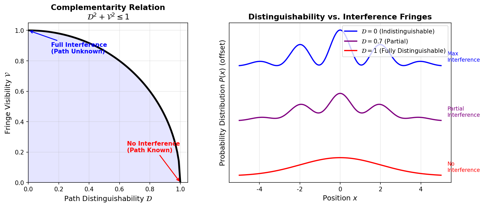
Fig. 3.7: Relationship between distinguishability and interference fringe visibility (complementarity). Left: The greater the path distinguishability \(\mathcal{D}\), the smaller the fringe visibility \(\mathcal{V}\). Right: When \(\mathcal{D} = 0\) (path unknown), interference is maximum; when \(\mathcal{D} = 1\) (path determined), interference vanishes; intermediate cases show a gradient.
🟡 Lina: But for now, let's summarize the two extreme cases as a general rule:
- When processes are in principle indistinguishable → add amplitudes (interference present)
- When processes are in principle distinguishable → add probabilities (no interference)
This rule is the heart of probability calculations in quantum mechanics.
✅ Comprehension Check: What is the criterion for deciding whether to "add amplitudes" or "add probabilities" in quantum mechanics?
Answer
When processes (paths) are in principle indistinguishable, add amplitudes (interference occurs); when in principle distinguishable, add probabilities (no interference occurs). The criterion is not whether observation was actually performed, but whether distinguishing information exists in principle.
✅ Comprehension Check: Even when "which slit the electron passed through was not observed," interference can still disappear. Under what circumstances does this occur?
Answer
Even without observation, if "information that could in principle distinguish the paths" remains somewhere in the environment (for example, a photon was scattered and its state would later reveal the path), then interference disappears. Whether the information is actually read out is irrelevant — the mere existence of the information destroys interference.
📝 Exercises:
- Photon wavelength and fringe visibility → Problem B-4. Conditions for Interference Maxima and Minima
3.5 The Collapse of the Classical Worldview — What to Abandon and What to Accept
🔵 Kai: Summarizing what we've covered... electrons are detected one at a time as particles, but if you don't ask "which way it went," they interfere. If you do ask, interference disappears. ...Honestly, I have no idea what's going on.
🟡 Lina: Feeling that you "don't understand" is the correct response. Feynman himself said: "I think I can safely say that nobody understands quantum mechanics." What's important is to clearly identify what cannot be explained by classical thinking.
🟡 Lina: Let me organize the three cases we've seen so far.
Table 3.2: Three cases in the double-slit experiment and the presence of interference
| Case | Path information | Probability composition rule | Interference fringes |
|---|---|---|---|
| No observation | Unknown (indistinguishable) | \(P_{12} = \lvert\phi_1 + \phi_2\rvert^2\) | Present |
| Observation with short-wavelength light | Determined (distinguishable) | \(P_{12}' = P_1 + P_2\) | Absent |
| Observation with long-wavelength light | Unknown (indistinguishable) | Approaches \(P_{12}\) | Recovers |
Testing the classical particle picture
🟡 Lina: First, let's test the following proposition:
Proposition A: Each electron passes through either slit 1 or slit 2.
If Proposition A is correct, then by the same logic as bullets, \(P_{12} = P_1 + P_2\) should hold. But the experimental result is \(P_{12} \neq P_1 + P_2\).
🔵 Kai: So Proposition A is wrong? The electron passes through both holes simultaneously?
🟡 Lina: The expression "passes through simultaneously" is also classical language, so it's not precise. What we can precisely say is:
If we assume "the electron passed through one or the other," we get a contradiction with experimental results.
We're not saying it "passed through both simultaneously" or "passed through neither." The question "which did it pass through?" itself has no meaning in this experimental situation.
⚪ Mei: "Has no meaning" — that's not saying we don't know the answer, but that the question itself is ill-posed?
🟡 Lina: Right. It's similar to asking "How old is the bachelor's wife?" There is no answer because the premise of the question doesn't hold.
Testing the classical wave picture
🔵 Kai: Then is the electron a wave? If it's a wave, interference would be natural.
🟡 Lina: If the electron were a classical wave, the detector should receive continuous energy. If you weaken the source, the arriving energy should continuously decrease. But in the experiment —
🔵 Kai: Oh, it always arrives with a "click" — one particle's worth of energy. There's never half a click.
🟡 Lina: Right. A classical wave cannot explain the fact that electrons "are detected as particles one at a time."
In summary:
Table 3.3: Comparison of explanatory power of classical particle and wave pictures
| Classical model | What it can explain | What it cannot explain |
|---|---|---|
| Particle picture | Detected one at a time | Interference fringes |
| Wave picture | Interference fringes | Detected one at a time |
Neither classical picture can fully describe the behavior of electrons.
The collapse of determinism
🔵 Kai: One more thing bothers me... can you predict where a single electron will arrive on the screen?
🟡 Lina: No.
🔵 Kai: Not at all?
🟡 Lina: Not at all. Even with the same apparatus, the same electron energy, fired in the same way, the arrival position differs every time. All that can be predicted is the probability distribution. No one can say "the next electron will arrive at \(x = 3.7\) mm on the screen."
⚪ Mei: In Newtonian mechanics, if the initial conditions are the same, the result is the same — it was deterministic. Does that not hold in quantum mechanics?
🟡 Lina: It does not hold. This is not about "we can't predict because our knowledge of initial conditions is insufficient." Even with initial conditions perfectly specified, the outcome is determined only probabilistically. This is the collapse of determinism in quantum mechanics.
🔵 Kai: But is it really "in principle unpredictable"? Couldn't there be some variable hidden inside the electron that we don't know about, and if we only knew it, we could predict?
✅ Comprehension Check: What is the "collapse of determinism" in quantum mechanics? How does it differ from uncertainty in classical mechanics (e.g., measurement errors in initial conditions)?
Answer
In quantum mechanics, even with initial conditions perfectly specified, individual measurement outcomes are determined only probabilistically. Classical uncertainty is epistemological — "we can't predict because our knowledge of initial conditions is insufficient" — but quantum indeterminacy is fundamental, a property of nature itself rather than a lack of knowledge.
⚪ Mei: So what Kai is asking is: "Maybe it only looks random on the surface, but there's actually some variable inside the electron that we don't know about, and if we knew it, the outcome would be determined?" The same structure as how a die's outcome is "in principle" determined by initial conditions in classical mechanics.
🟡 Lina: Excellent question. That "invisible information" is called a hidden variable in physics. In fact, Einstein thought exactly this. "God does not play dice," he said. The question was experimentally settled by Bell's inequality, which we'll cover in detail in Ch. 23. Let me just give you the conclusion: nature really does play dice — that's what current experimental evidence indicates.
🔵 Kai: Even Einstein couldn't accept it, but it was settled by experiment...? But how can you experimentally confirm that "there are no hidden variables"? Proving that something invisible "doesn't exist" seems really hard.
🟡 Lina: That's exactly where Bell's genius lies. He showed that "if hidden variables exist, a certain inequality must hold," then checked experimentally whether that inequality is violated. We'll cover the details in Ch. 23.
🔵 Kai: "An inequality that must hold if they exist" gets violated by experiment... then you can say they "don't exist." Proof by contradiction. But how can you derive an "inequality that must hold" without knowing what's inside the hidden variable? Can a universal consequence really follow from just the assumption of existence without specifying the concrete form?
🟡 Lina: Good question. Intuitively it goes like this — you don't specify the "content" of the hidden variable, but you impose just the condition that "measurement results at distant locations don't instantaneously influence each other" (locality). Then an upper bound emerges on the correlations between measurement results of two separated particles. Quantum mechanics predicts correlations exceeding that upper bound — so the experiment can distinguish them.
🔵 Kai: Just assuming locality produces an upper bound on correlations... then indeed you don't need to know the "content."
🟡 Lina: Right. Bell's cleverness is that even without knowing the specific content of the hidden variables, the inequality can be derived from just the assumption that "local hidden variables exist." That is, from just two assumptions — "hidden variables exist" + "locality" — the inequality follows, and quantum mechanics violates it — so at least one of the assumptions must be wrong. The specific form doesn't matter. We'll go through the details carefully in Ch. 23; for now, just remember the structure that "it's settled by proof by contradiction."
⚪ Mei: So even without knowing the content, the assumption of "existence" alone produces consequences, making experimental refutation possible. The structure of proof by contradiction holds beautifully. The logical structure of Bell's argument is: "assumption (hidden variables + locality) → inequality → violated by experiment → at least one assumption is false" — precisely proof by contradiction. Since the inequality follows from just existence and locality without specifying the concrete content of hidden variables, the refutation is universally valid.
The collapse of realism
🟡 Lina: There's one more, deeper issue. Classical physics implicitly assumed the following:
Realism: Physical quantities always have definite values regardless of whether they are measured. Measurement is merely the act of "reading" an already-existing value.
🔵 Kai: Isn't that obvious? The moon exists even when nobody's looking at it, right?
🟡 Lina: For macroscopic objects like the moon, yes, indeed. But for "which slit the electron passed through," this thinking breaks down.
What the double-slit experiment demonstrates is:
"Which way it went" is not determined unless measured. Measurement does not "read an already-existing value" but rather is the act of making the value definite.
🔵 Kai: So the electron's position or velocity aren't determined before you measure them?
🟡 Lina: At least for "which slit it passed through," it is not determined before measurement. And this isn't limited to the electron's path. In quantum mechanics generally, the classical assumption that "all physical quantities have definite values at each instant" is abandoned. A physical state is not defined as "a list of values of all physical quantities" but as "something that gives the probability distribution of what you'd get if you measured."
⚪ Mei: A state is not "a list of values" but "a prescription for probability distributions" — the worldview changes fundamentally.
✅ Comprehension Check: What is "realism" in classical physics? How does the double-slit experiment deny it?
Answer
Classical realism is the assumption that "physical quantities always have definite values regardless of whether they are measured." In the double-slit experiment, "which slit the electron passed through" is not determined before measurement, and assuming a definite path contradicts the experimental result (\(P_{12} \neq P_1 + P_2\)). Measurement does not read a pre-existing value but rather makes the value definite.
⚪ Mei: So the "path not being definite" we saw in the double slit is a principle that pervades all of quantum mechanics.
Conclusions of this chapter
🟡 Lina: Let's organize what we learned from the double-slit experiment.
- Probability amplitude: The arrival probability of an electron is given by the absolute value squared \(|\phi|^2\) of a complex probability amplitude \(\phi\)
- Superposition: When multiple paths exist, add the amplitudes of indistinguishable paths, then square
- Effect of observation: When information distinguishing paths exists, the interference term vanishes, and probabilities simply add
- Collapse of determinism: Where an individual electron will arrive is in principle unpredictable. Only the probability distribution can be predicted
- Revision of realism: It is not possible to attribute a definite value to a physical quantity that has not been measured
🔵 Kai: It feels like the way I see the world is about to change fundamentally...
🟡 Lina: Yes. But what's important is that this is not philosophical speculation — it's a conclusion drawn from experimental facts. This is how nature is.
⚪ Mei: So what we've seen in this chapter is that the rule "add probability amplitudes then square" correctly reproduces experimental facts, and that it's precisely the state where "which way it went" is not definite that produces interference.
🟡 Lina: Right. And conversely, a classical worldview that assigns definite values to physical quantities before measurement cannot explain this experiment. If we formulate this rule mathematically with precision, we'll be able to quantitatively predict the behavior of atoms. In the next chapter, we'll see this organized as three fundamental rules by Feynman.
✅ Comprehension Check: What conditions are necessary to claim "the electron passed through slit 1"? And what happens when those conditions are met?
Answer
To claim "the electron passed through slit 1," a measurement that identifies the path is required (e.g., scattering a photon near the slit). However, performing that measurement causes the interference fringes to disappear, and the probability distribution changes to \(P_{12} = P_1 + P_2\). "Knowing which way it went" and "seeing interference fringes" are mutually incompatible.
3.6 Supplement: Actual Experiments and History
🟡 Lina: Finally, let me add some historical notes about this experiment.
When Feynman wrote about this double-slit experiment in his textbook in the 1960s, the experiment of sending electrons one at a time and observing interference fringes had not yet been realized. Feynman explicitly noted that "this experiment has never been done in just this way."
However, in 1989, Akira Tonomura and colleagues at Hitachi used an electron biprism to successfully film the gradual formation of interference fringes as electrons were sent one at a time. The result perfectly matched Feynman's thought experiment prediction.
🔵 Kai: A thought experiment was verified 30 years later.
🟡 Lina: This is precisely where the power of physics models lies. They can predict the results of experiments that haven't been performed yet. And those predictions are later confirmed by experiment. This is the strength of scientific models that possess "falsifiability."
⚪ Mei: So quantum mechanics is trusted because its predictions have been confirmed by experiment — and if they had failed, corrections would have been needed.
🟡 Lina: Exactly. And quantum mechanics has not yet encountered such a falsification. That's why it is trusted as "the best current hypothesis."
Preview of the Next Chapter
🟡 Lina: In this chapter, through the double-slit experiment, we discovered the rules: "add probability amplitudes" and "for indistinguishable processes add amplitudes, for distinguishable processes add probabilities."
But questions remain:
- How exactly do we calculate the probability amplitude \(\phi\)?
- What happens when there are "three or more paths"?
- When passing through "intermediate paths," how do amplitudes combine?
In the next chapter (Ch. 4), we'll refine the "add amplitudes" and "multiply amplitudes" rules glimpsed in this chapter into a more general and precise form, and together with one more law, formulate them as three fundamental laws of probability amplitudes. With just these three laws organized by Feynman, we'll be able to calculate probabilities for any quantum phenomenon.
Practice Problems
📝 Exercises:
- Derivation of double-slit interference conditions → Problem M-4. Understanding the Disappearance of Interference through "Conditional Decomposition of Probability"
- Sign of interference term and bright/dark fringes → Problem B-1. Calculation of Interference Terms
- Photon wavelength and fringe visibility → Problem B-4. Conditions for Interference Maxima and Minima
References
- R. P. Feynman, R. B. Leighton, M. Sands, The Feynman Lectures on Physics, Vol. III, Ch. 1 "Quantum Behavior", Ch. 3 "Probability Amplitudes" (Addison-Wesley, 1965)
- J. J. Sakurai, J. Napolitano, Modern Quantum Mechanics, 3rd ed., Ch. 1 (Cambridge University Press, 2021)
- 清水明『新版 量子論の基礎 — その本質のやさしい理解のために』(サイエンス社, 2004), 第 2 章「基本的枠組み」
- 広江克彦『趣味で量子力学』第 3 章「二重スリットの実験」
- A. Tonomura, J. Endo, T. Matsuda, T. Kawasaki, H. Ezawa, "Demonstration of single-electron buildup of an interference pattern", American Journal of Physics 57, 117–120 (1989)
Feedback on this page
Let us know if something was unclear, incorrect, or could be improved.