Chapter 1: Why Do Planets Move the Way They Do? — The Birth of Newtonian Mechanics
Story so far: In the Prologue, we confirmed three things. (1) All physics models are merely hypotheses. (2) Writing them in mathematical form enables quantitative predictions and makes them falsifiable. (3) The motivations for creating models come in two varieties: "practical necessity" and "pure curiosity." Starting from this chapter, we'll look at concrete examples. The first example is one of the most successful models in human history—Newton's universal gravitation.
Goals of this chapter
- Relive the story of how the methodology of physics—"explaining many phenomena in a unified way from a single model"—was established
- Understand what motivated Newton's model of universal gravitation, what it can predict, and what it cannot explain
1.1 Motivation: Why Do Planets Move the Way They Do?
🟡 Lina: Now then, in the Prologue we discussed how "models are hypotheses" and "writing them in equations makes them testable." Starting today, we'll look at specific models. The first question is this: Why do planets move the way they do?
🔵 Kai: They orbit around the Sun, right? I know that much.
🟡 Lina: Yes. But "they orbit" is an observational fact—it doesn't explain why they orbit. The person who answered this "why" with a single unified model was Isaac Newton.
⚪ Mei: There were people who described planetary motion before Newton, right? Like Kepler.
🟡 Lina: Good catch. To understand Newton's model, we first need to know about Kepler's work. Let me organize the differences between their contributions.
Table 1.1: Comparison of Kepler's and Newton's work
| Kepler | Newton | |
|---|---|---|
| Question | What is happening? | Why does it happen? |
| Method | Extract patterns from observational data | Derive phenomena from principles (a model) |
| Achievement | 3 empirical laws | Law of universal gravitation |
| Scope of explanation | Planetary orbits only | Unified from falling objects on Earth to celestial bodies |
| Proportionality constant | "This relationship exists" | "The constant's identity is the Sun's mass" |
🔵 Kai: The difference in "scope of explanation" in this table is amazing. Kepler only covers planets, but Newton includes phenomena on Earth too?
🟡 Lina: That's right. "Explaining a broader range of phenomena in a unified way from a single model"—that's the power of physics models. We'll see this throughout this entire chapter.
✅ Comprehension Check: What new question did Newton answer that Kepler's work did not?
Answer
The question of "why do planets move the way they do?"—a question about the cause (why) of motion. Kepler only described "what is happening."
1.2 Kepler's Three Laws — Describing "What Is Happening"
🟡 Lina: In the early 17th century, Johannes Kepler analyzed the vast astronomical observation data of Tycho Brahe and discovered three regularities in planetary motion.
🔵 Kai: I learned these in high school! Let me think...
🟡 Lina: Let's go through them one by one. I've illustrated all three laws in Fig. 1.1 "Illustration of Kepler's three laws", so check the corresponding parts as you hear each explanation.
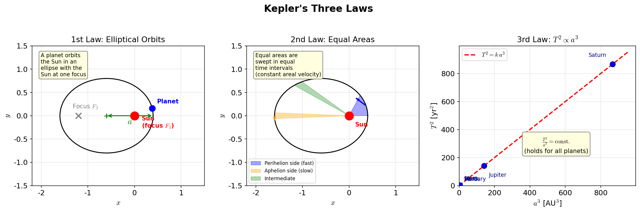
Fig. 1.1: Illustration of Kepler's three laws. First law: elliptical orbits and focal points. Second law: constant areal velocity (faster when closer to the Sun). Third law: the relationship \(T^2 \propto a^3\).
First Law: Elliptical Orbits
🟡 Lina: Planets move along ellipses with the Sun at one focus.
🔵 Kai: Not circles but ellipses, right?
🟡 Lina: That's right. At the time, the common belief was that "celestial bodies move in perfect circles." Kepler was faithful to the data and concluded they were ellipses. This took great intellectual courage.
Second Law: Equal Areas
🟡 Lina: The line segment connecting a planet to the Sun sweeps out equal areas in equal time intervals. In other words, when closer to the Sun the planet moves faster, and when farther away it moves slower.
🔵 Kai: Why does it go faster when it's closer?
🟡 Lina: As a rough image, think about how the area of a triangle is "base × height ÷ 2." When closer to the Sun, the base (distance) becomes shorter, so to sweep the same area, the height (speed) needs to compensate. Strictly speaking, the direction of velocity also matters, but the qualitative conclusion that "closer means faster" is correct.
🔵 Kai: Ah, so because the base is shorter, the height—meaning the speed—has to make up for it or the area won't be enough. But why is the areal velocity constant? Is it just coincidence? It seems like other laws—say "areal velocity proportional to distance"—could also work.
⚪ Mei: At this stage, it's just a description saying "this regularity exists." The "why it's constant" will only be explained through Newton's model.
🟡 Lina: Exactly. The "why" of constant areal velocity is a conclusion derived from Newton's model. For now, just note the fact that "this pattern exists."
🟡 Lina: In equation form, let \(dA\) be the tiny area swept by the line segment connecting the planet and Sun during a very short time \(dt\) (\(d\) is a symbol meaning "infinitesimal," and \(dA/dt\) is "the rate of change of \(A\)"—the same notation as \(dx/dt\) representing velocity that you learned in high school). \(\frac{dA}{dt}\) is "the area swept per unit time"—this is called the areal velocity. The second law states that this areal velocity has the same value at every instant:
Third Law: Harmonic Law
🟡 Lina: The square of a planet's orbital period \(T\) is proportional to the cube of the semi-major axis \(a\) of its orbit. The semi-major axis is half the length of the longest diameter (major axis) of the ellipse. As the ellipse approaches a circle, the semi-major axis equals the radius of the circle.
🔵 Kai: That's a really elegant relationship, isn't it?
🟡 Lina: It is. But what's important here is that Kepler's three laws only describe "what is happening" and do not explain "why it happens."
🔵 Kai: True—being told "they trace ellipses" doesn't tell us why they're ellipses.
⚪ Mei: Right. Why is the areal velocity constant? Why \(T^2 \propto a^3\)? Kepler's laws are descriptions of "what is happening," and the reasons are a separate matter.
🟡 Lina: The person who answered that "why" was Newton.
✅ Comprehension Check: Whose observational data did Kepler analyze to discover his three laws?
Answer
The vast astronomical observation data of Tycho Brahe.
✅ Comprehension Check: How do you write Kepler's third law as an equation?
Answer
\(T^2 \propto a^3\) (the square of the orbital period is proportional to the cube of the semi-major axis of the orbit).
1.3 Newton's Universal Gravitation — A Model for "Why It Happens"
🟡 Lina: Newton's idea was surprisingly simple. All objects exert a mutually attractive force on each other. The magnitude of that force is:
Here \(m_1\), \(m_2\) are the masses of the two objects, \(r\) is the distance between them, and \(G\) is the gravitational constant (\(G \approx 6.67 \times 10^{-11}\;\mathrm{m^3\,kg^{-1}\,s^{-2}}\)).
🔵 Kai: I learned this in high school, but looking at it again, it really is simple.
🟡 Lina: Yes. But from this single equation, all three of Kepler's laws can be derived. Let's actually do it.
Derivation of Kepler's Third Law (Circular Orbit Approximation)
🔵 Kai: Really? From just that simple equation?
🟡 Lina: To keep things simple, let's first approximate the planet's orbit as a circle. Suppose a planet of mass \(m\) orbits a Sun of mass \(M\) in a circular orbit of radius \(r\).
🔵 Kai: Is it okay to use a circle instead of an ellipse?
🟡 Lina: Proving it for a general ellipse requires university-level differential equations. But a circle is a special case of an ellipse, and the conclusion \(T^2 \propto a^3\) holds exactly for ellipses too. First, let's grasp the essence.
🟡 Lina: I've shown this situation in Fig. 1.2 "The relationship between universal gravitation and centripetal force in a circular orbit". To maintain circular motion, a centripetal force (a force directed toward the center) is needed. As you learned in high school, the centripetal force required for an object of mass \(m\) moving at speed \(v\) in a circle of radius \(r\) is:
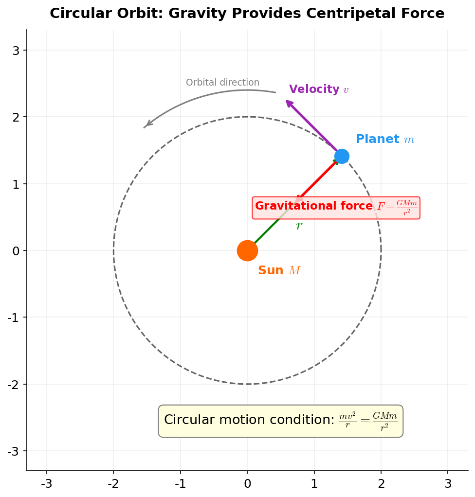
Fig. 1.2: The relationship between universal gravitation and centripetal force in a circular orbit. The planet moves along its circular orbit at speed \(v\), and the gravitational force \(F = GMm/r^2\) from the Sun provides the centripetal force.
🔵 Kai: And the universal gravitation is what provides that centripetal force, right?
🟡 Lina: Exactly. Since universal gravitation provides the centripetal force, we set them equal:
Dividing both sides by \(m\):
Rearranging:
⚪ Mei: Everything up to here is within the high school curriculum.
🟡 Lina: Next, let's rewrite the speed \(v\) using the orbital period \(T\). The circumference is \(2\pi r\), so:
Substituting this into \(v^2 = GM/r\):
Computing the square on the left side:
We want to isolate \(T^2\) on the left, so multiply both sides by \(T^2\) (eliminating the denominator on the left):
To eliminate the \(r\) in the denominator on the right, multiply both sides by \(r\) (eliminating the denominator on the right):
Solving for \(T^2\):
🔵 Kai: Wow! The right side is all constants. So \(T^2 \propto r^3\) comes out! But wait—this is for circular orbits, right? Does it really hold for ellipses too?
🟡 Lina: Good question. For general elliptical orbits, \(T^2 \propto a^3\) holds exactly—but the proof requires knowledge of differential equations, so for now accept that "a circle is a special case of an ellipse, and the conclusion is the same for ellipses." In a circular orbit, the radius \(r\) equals the semi-major axis \(a\), so this is precisely Kepler's third law \(T^2 \propto a^3\). I've summarized the flow of the entire derivation in Fig. 1.3 "Derivation steps for Kepler's third law".
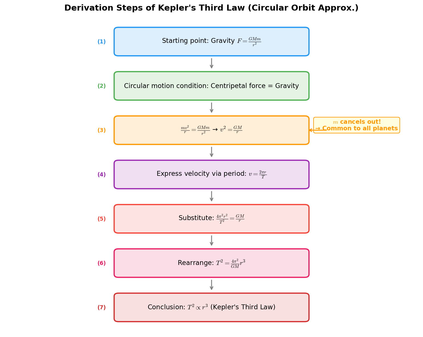
Fig. 1.3: Derivation steps for Kepler's third law. Starting from universal gravitation, using only the condition for circular motion and rewriting the velocity, we obtain \(T^2 \propto r^3\). The fact that the planet's mass \(m\) cancels in step (3) is the key to "a proportionality constant common to all planets."
🟡 Lina: Moreover, we can see that the proportionality constant \(4\pi^2/(GM)\) is determined solely by the Sun's mass \(M\). In other words, a proportionality constant common to all planets automatically emerges from Newton's model.
🔵 Kai: "Common to all planets"—is that because the planet's mass \(m\) canceled out?
🟡 Lina: Exactly. The planet's mass disappeared when we divided both sides by \(m\) at the beginning. So the proportionality constant is determined only by the Sun's mass \(M\).
⚪ Mei: Kepler only said "\(T^2 \propto a^3\) holds," but Newton tells us both "why it holds" and "what the proportionality constant is."
🟡 Lina: This is the "power of a model." Rather than memorizing individual phenomena one by one, you can logically derive many phenomena from a single principle.
📝 Exercises:
- Derive Kepler's third law from universal gravitation → Problem M-1. Derivation of Kepler's Third Law
✅ Comprehension Check: Write Newton's law of universal gravitation. What does each symbol mean?
Answer
\(F = G\frac{m_1 m_2}{r^2}\). \(m_1, m_2\) are the masses of the two objects, \(r\) is the distance between them, and \(G\) is the gravitational constant.
✅ Comprehension Check: What is the significance of Newton's model relative to Kepler's three laws?
Answer
Three independent regularities (Kepler's three laws) can all be derived from a single model—universal gravitation. Furthermore, the physical meaning of the proportionality constant (determined by the Sun's mass) becomes clear.
1.4 Newton's Cannonball — Unifying the Terrestrial and Celestial
🟡 Lina: Another revolutionary aspect of Newton's model is that it unified terrestrial and celestial phenomena.
🔵 Kai: The force that drops an apple is the same force keeping the Moon in orbit?
🟡 Lina: Yes. Newton conducted a famous thought experiment (Fig. 1.4 "Newton's cannonball thought experiment"). Fire a cannonball horizontally from a mountaintop. If you fire it weakly, it traces a parabola and hits the ground. Fire it harder, and it lands farther away. Fire it even harder—
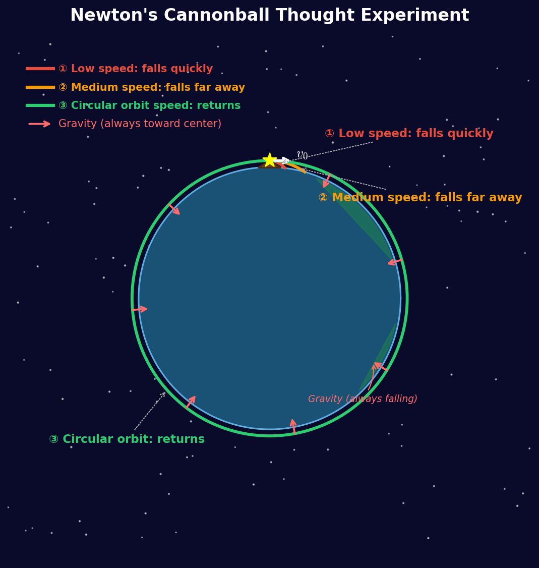
Fig. 1.4: Newton's cannonball thought experiment. As the initial speed of a cannonball fired horizontally from a mountaintop increases, the trajectory changes from immediate fall → distant fall → circular orbit (returns after one revolution). The upper right shows a close-up near the launch point.
🔵 Kai: Um... since the Earth is round, the ground curves away too, right? Could it be that it keeps falling but never reaches the ground?
🟡 Lina: Exactly! If fired fast enough, the cannonball keeps falling along the curvature of the Earth, goes all the way around, and comes back. In other words, it "enters orbit." The Moon is doing precisely this—it's "continuously falling." It just has enough sideways velocity that the ground curves away before it can reach the surface. As a result, the Moon keeps orbiting the Earth.
⚪ Mei: So falling and orbital motion are different manifestations of the same phenomenon.
🔵 Kai: Falling but not falling... that's a strange feeling. But how fast do you need to fire it to reach the state of "falling continuously but never reaching the ground"? Intuitively it seems like you'd need an incredible speed.
🟡 Lina: Good question. To enter orbit near the Earth's surface requires about 7.9 km/s (the first cosmic velocity)—about 23 times the speed of sound. The equation \(v^2 = GM/r\) we derived earlier is the condition for a circular orbit, so substituting Earth's mass for \(M\) and Earth's radius \(R_E\) for \(r\) gives you this value.
🔵 Kai: 23 times the speed of sound... that really is incredible.
🟡 Lina: But what I want to confirm here is something even more important. Let's do a quantitative check on whether "terrestrial gravity" and "the force keeping the Moon in orbit" really obey the same law. The Moon is at a distance of about \(r = 3.84 \times 10^8\;\mathrm{m}\) from Earth, with an orbital period of about \(T = 27.3\) days \(\approx 2.36 \times 10^6\;\mathrm{s}\). The Moon's orbital speed is:
The centripetal acceleration the Moon experiences is:
🔵 Kai: That's much smaller than \(g = 9.8\;\mathrm{m/s^2}\) at the surface. Is it weaker because the Moon is far away? I wonder how much weaker it should be.
🟡 Lina: Good question. If gravity is inversely proportional to the square of the distance, we can calculate the acceleration at the Moon's position. Earth's radius is about \(R_E \approx 6.4 \times 10^6\;\mathrm{m}\), so the distance to the Moon, \(3.84 \times 10^8\;\mathrm{m}\), is about \(60\) times Earth's radius. Therefore:
🔵 Kai: Whoa, they match exactly!
⚪ Mei: The value calculated from the Moon's orbit and the value obtained by dividing surface gravity by the square of the distance agree... this is hard to dismiss as coincidence.
🟡 Lina: This agreement cannot be coincidental. To summarize, two completely independent calculations—"the acceleration determined from the Moon's orbital data" and "the acceleration obtained by extrapolating surface \(g\) using the inverse-square law"—both give \(0.00272\;\mathrm{m/s^2}\). The force that drops an apple and the force that keeps the Moon in orbit are the same universal gravitation. Until then, it was believed that "the celestial realm" and "the terrestrial realm" operated under different laws. Newton unified them with a single model.
✅ Comprehension Check: What "unification" does Newton's cannonball thought experiment demonstrate?
Answer
That the force dropping an apple (terrestrial gravity) and the force keeping the Moon in orbit (celestial force) are the same universal gravitation. It unified terrestrial and celestial phenomena with a single model.
1.5 The Predictive Power of a Model — The Discovery of Neptune
🟡 Lina: The most dramatic demonstration of Newton's model's power was the discovery of Neptune.
🔵 Kai: Neptune?
🟡 Lina: In the mid-19th century, astronomers noticed that Uranus's orbit deviated slightly from the predictions of Newton's model.
⚪ Mei: It's possible the model was wrong.
🟡 Lina: Right—there were two possibilities. (1) Newton's model is wrong. (2) An undiscovered celestial body is influencing Uranus.
🟡 Lina: The Frenchman Urbain Le Verrier and the Englishman John Couch Adams assumed (2) and calculated the position of the unknown planet backward from Newton's model (Fig. 1.5 "Conceptual diagram of Neptune's discovery"). Then in 1846, when a telescope was pointed at the position Le Verrier predicted—
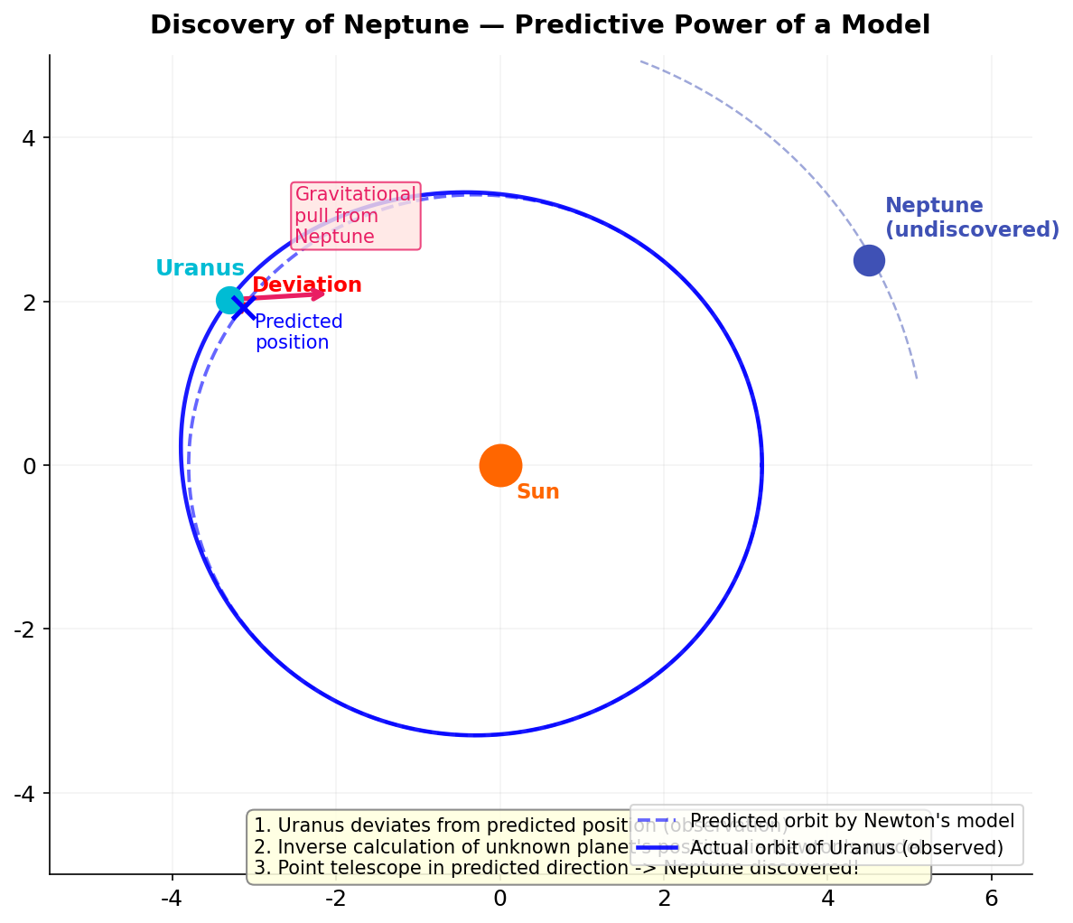
Fig. 1.5: Conceptual diagram of Neptune's discovery. The actual orbit of Uranus (solid line) deviates from the predicted orbit from Newton's model (dashed line). Assuming the cause of this deviation to be "the gravity of an undiscovered planet," its position was calculated backward, leading to the discovery of Neptune.
🔵 Kai: It was actually there!?
🟡 Lina: It was. Neptune. Within just 1 degree of the predicted position.
📝 Exercises:
- Estimate Neptune's mass from the orbital deviation → Problem B-1. Estimating the Mass of Neptune
⚪ Mei: This is the power of "quantitative prediction." Not "there might be a planet somewhere," but "it's in this direction at this position"—the equations told us.
🟡 Lina: Remember how in the Prologue I said "writing in equations makes quantitative verification possible"? The discovery of Neptune is precisely a real-world example of that.
✅ Comprehension Check: What did the discovery of Neptune demonstrate about Newton's model?
Answer
The model's quantitative predictive power. The position of an unknown planet was calculated backward from equations, and Neptune was actually discovered at the predicted position.
✅ Comprehension Check: What were the two possibilities considered for Uranus's orbital deviation?
Answer
(1) Newton's model is wrong. (2) An undiscovered celestial body is influencing Uranus.
1.6 Gravitational Potential and the Poisson Equation
🟡 Lina: Let me now rewrite Newton's model in a more modern form. We'll need this in later chapters.
🟡 Lina: We assign a number to each point in space representing the "gravitational height"—the gravitational potential \(\Phi(\mathbf{r})\). \(\mathbf{r}\) is a vector representing position in space (bold indicates a vector by convention, meaning the same thing as \(\vec{r}\) used in high school). \(\Phi\) is just a number (scalar) determined at each position.
🔵 Kai: "Gravitational height"—is that like the elevation of a mountain?
🟡 Lina: Good intuition. The higher the elevation, the greater the potential energy, right? Similarly, places where \(\Phi\) is large have higher gravitational energy. And objects experience a force toward lower \(\Phi\)—that is, in the "downhill" direction.
🟡 Lina: Written as an equation, the force on a particle of mass \(m\) is
Here \(\nabla\Phi\) (read "nabla \(\Phi\)") is a quantity called the gradient. Think of contour lines on a topographic map—look at Fig. 1.6 "Contour map of gravitational potential". Where contour lines are packed closely together, the slope is steeper, right? The gradient is "a vector pointing in the direction of steepest ascent, with magnitude equal to that slope." Because of the minus sign, the force acts in the direction where \(\Phi\) decreases—the downhill direction. The precise definition of the gradient is covered in General Relativity Ch. 1, but for now think of it as "the direction perpendicular to contour lines going downhill, and its steepness."
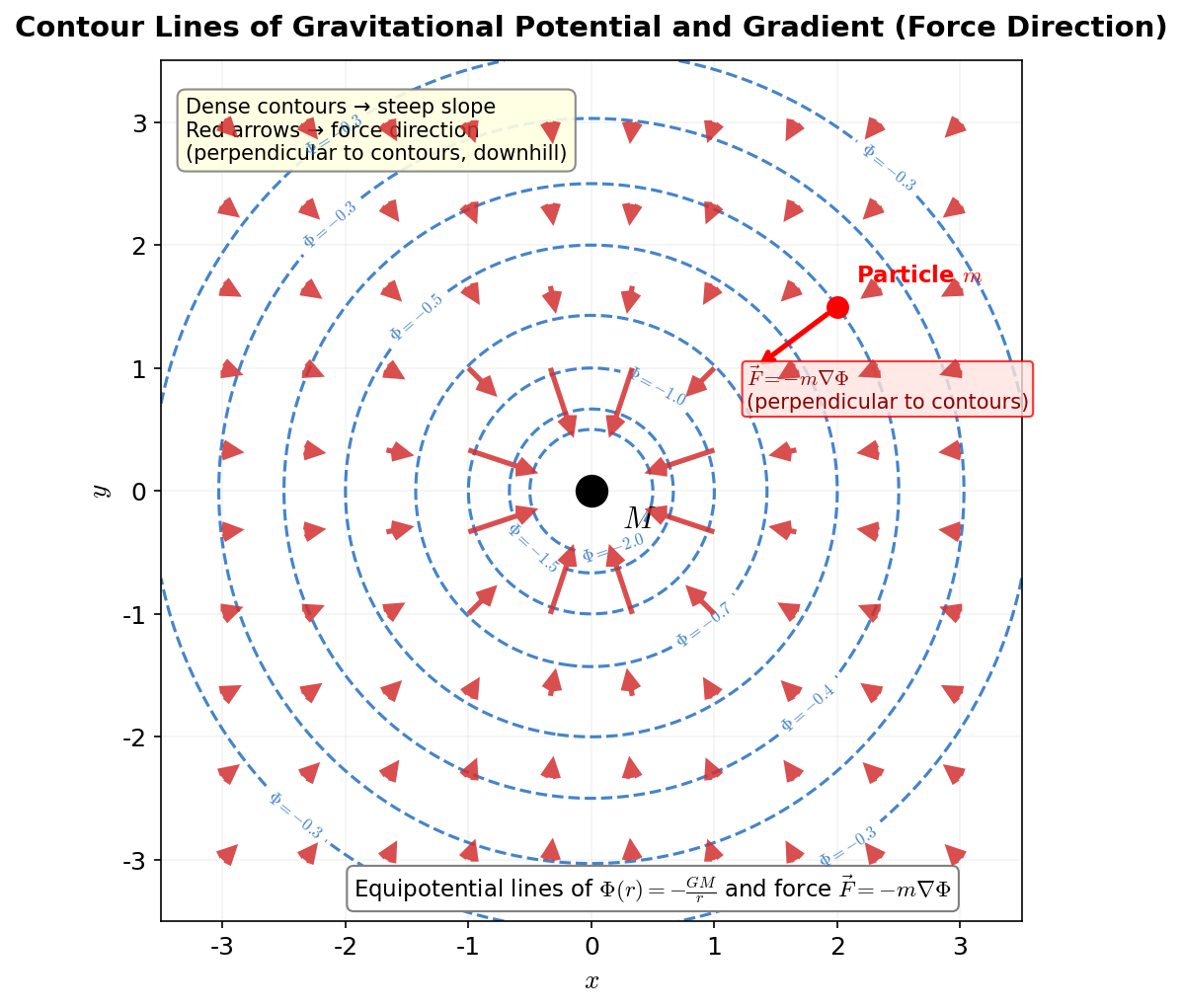
Fig. 1.6: Contour map of gravitational potential. Blue curves are equipotential lines (lines where \(\Phi\) is constant), and red arrows indicate the direction of force \(\vec{F} = -m\nabla\Phi\). The more densely packed the contour lines, the "steeper the slope" and the stronger the force. The force is always perpendicular to contour lines, pointing toward lower \(\Phi\) (toward the center).
⚪ Mei: So instead of writing the force directly, you first create a "height map" and then read off the force from it.
🟡 Lina: Exactly. Now let's think about what form \(\Phi\) must have for \(\mathbf{F} = -m\nabla\Phi\) to reproduce universal gravitation. Let's consider the spherically symmetric case—where \(\Phi\) depends only on the distance \(r\) from the center. "Depends only on \(r\)" means that as long as you're at the same distance \(r\), the value of \(\Phi\) is the same regardless of direction. In terms of a contour map, this is the situation where contour lines are concentric circles.
🔵 Kai: With concentric contour lines, the only uphill direction is radially outward from the center, right? Moving sideways doesn't change the height.
🟡 Lina: Exactly. Moving in the transverse direction without changing the distance from the center leaves \(\Phi\) unchanged—the transverse slope is zero. So the "steepest ascent direction" can only be the \(r\) direction (radially outward from center). As a result, the gradient is only the slope in the \(r\) direction. So the magnitude of the gradient can be written as \(|\nabla\Phi| = \frac{d\Phi}{dr}\) (directed in the direction of increasing \(r\)).
🔵 Kai: I follow so far. And now we determine \(\Phi\) so that this gradient matches universal gravitation, right?
🟡 Lina: Right. The magnitude of universal gravitation is \(F = GMm/r^2\) directed toward the center (direction of decreasing \(r\)). Taking the \(r\) direction (radially outward from center) as positive, the \(r\)-component of the force is \(F_r = -GMm/r^2\) (negative because it points toward center). Meanwhile, the \(r\)-component of \(\mathbf{F} = -m\nabla\Phi\) is \(F_r = -m\frac{d\Phi}{dr}\). Setting these equal: \(-m\frac{d\Phi}{dr} = -\frac{GMm}{r^2}\). Dividing both sides by \(-m\): \(\frac{d\Phi}{dr} = \frac{GM}{r^2}\).
⚪ Mei: "Differentiating \(\Phi\) with respect to \(r\) gives \(GM/r^2\)"—so the inverse operation gives us \(\Phi\).
🟡 Lina: Exactly. Integrating this with respect to \(r\)—meaning "what function \(\Phi(r)\) gives \(GM/r^2\) when differentiated?"—is the reverse operation. We use the formula from high school: \(\int r^n\,dr = \frac{r^{n+1}}{n+1}\) (\(n \neq -1\)). "Integrating" means "the inverse of differentiation"—finding the function \(\Phi(r)\) whose derivative is \(GM/r^2 = GM \cdot r^{-2}\). Since \(GM\) is a constant, we can pull it outside the integral: \(\int GM \cdot r^{-2}\,dr = GM \int r^{-2}\,dr\). Substituting \(n = -2\) into the formula gives \(n+1 = -2+1 = -1\), so \(\int r^{-2}\,dr = \frac{r^{-1}}{-1} = -\frac{1}{r}\). Let's verify—differentiating \(-1/r = -r^{-1}\) with respect to \(r\) gives \(-(-1)r^{-2} = r^{-2} = 1/r^2\), which indeed returns us to the original. Therefore \(\Phi = GM \times (-1/r) + C = -GM/r + C\). Here \(C\) is the integration constant—since indefinite integrals have the freedom that "adding a constant still gives the same derivative," one undetermined constant always remains (check: \(d(-GM/r + C)/dr = GM/r^2\), and \(C\) vanishes upon differentiation). This \(C\) is determined by the condition "at infinity, \(\Phi = 0\)." As \(r \to \infty\), \(-GM/r \to 0\), so \(\Phi(\infty) = 0 + C = C\). For this to be zero, we need \(C = 0\).
🔵 Kai: Why are we allowed to set it to zero at infinity?
🟡 Lina: Only differences in potential have physical meaning—since force is determined by the slope (derivative) of \(\Phi\), adding a constant to all of \(\Phi\) doesn't change the force. So you can place the reference point anywhere, but "zero influence infinitely far from mass" is natural, so setting infinity to zero is the convention.
🔵 Kai: So it has a minus sign. \(\Phi\) takes negative values?
🟡 Lina: Yes. The minus sign means that \(\Phi\) gets lower as you approach the mass—it takes the shape of "going downhill toward the bottom of a valley." This is consistent with objects being attracted, right?
🔵 Kai: Ah, it really does come out from the calculation.
🟡 Lina: To summarize, integrating \(\frac{d\Phi}{dr} = \frac{GM}{r^2}\) and setting \(\Phi = 0\) at infinity gives:
🔵 Kai: Since it's negative, \(\Phi\) gets deeper as you approach the mass.
🟡 Lina: Exactly. Look at the graph in Fig. 1.7 "Graph of gravitational potential \(\Phi(r) = -GM/r\). \(\Phi\) gets deeper (valley bottom) as you approach mass \(M\). The force \(F = -m\,d\Phi/dr\) points in the direction of decreasing \(r\)"—it has the shape of "a slope heading toward the bottom of a valley" where \(\Phi\) gets deeper as \(r\) decreases.
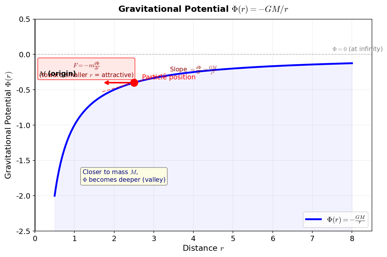
Fig. 1.7: Graph of gravitational potential \(\Phi(r) = -GM/r\). \(\Phi\) gets deeper (valley bottom) as you approach mass \(M\). The force \(F = -m\,d\Phi/dr\) points in the direction of decreasing \(r\)—that is, downhill. The slope of the tangent line corresponds to the magnitude of the force.
🟡 Lina: Now let me take one step further. The \(\Phi = -GM/r\) we just found was the potential "when mass \(M\) is at a single point." So how is \(\Phi\) determined when mass is distributed throughout space? To write that answer, let me first introduce a new tool. The Laplacian \(\nabla^2\) (read "nabla squared")—an operation that measures the spatial "curvature" of the potential. In one dimension it would be \(d^2\Phi/dx^2\)—the three-dimensional version of the "second derivative."
🔵 Kai: The second derivative is the thing that represents the "concavity" of a function, right?
🟡 Lina: Yes. Recall the sign of the second derivative. The graph of \(y = x^2\) is concave up (valley shape) with \(d^2y/dx^2 = 2 > 0\) (positive). \(y = -x^2\) is concave down (hilltop shape) with \(d^2y/dx^2 = -2 < 0\) (negative). So concave up (valley) means positive second derivative, concave down (hilltop) means negative. For example, at a valley bottom, \(\Phi\) at that point is lower than the values to either side—meaning "less than the average of surrounding values." Conversely, at a hilltop it's higher than the surroundings. Roughly speaking, the Laplacian measures "how much \(\Phi\) at a point deviates from the average of its surroundings."
🔵 Kai: I see—it quantifies "whether a point is dipped below or sticking above the surroundings."
🟡 Lina: Right. Using this tool, the relationship between mass distribution and potential can be written neatly. Stating the conclusion first: "the Laplacian at each point is proportional to the mass density at that point." This expressed as an equation is the Poisson equation:
Here \(\rho\) (rho) is the mass density—mass per unit volume. The coefficient \(4\pi\) comes from the geometry of spherical symmetry; its derivation is done in General Relativity Ch. 1.
⚪ Mei: "The potential is concave where matter exists"—that's what the Poisson equation is saying.
🔵 Kai: What does the "three-dimensional version" look like concretely?
🟡 Lina: It's the sum of second derivatives in each direction (\(x\), \(y\), \(z\))—\(\nabla^2\Phi = \frac{\partial^2\Phi}{\partial x^2} + \frac{\partial^2\Phi}{\partial y^2} + \frac{\partial^2\Phi}{\partial z^2}\). The \(\partial\) (rounded d) is the symbol for partial derivatives, meaning "differentiate with respect to one direction while holding the other variables fixed." For example, \(\frac{\partial^2\Phi}{\partial x^2}\) means "fix \(y\) and \(z\) and look at the curvature in the \(x\) direction only." Adding those up for all 3 directions gives the Laplacian. The detailed treatment of partial derivatives is in General Relativity Ch. 1, but for now think of it as "the sum of curvatures in all directions."
🟡 Lina: Let me confirm one thing here. The graph of \(\Phi = -GM/r\) that we found earlier is clearly curved. You might think "then the Laplacian isn't zero, is it?" But the "curvature" we're talking about here isn't the curvature of the one-dimensional graph (\(d^2\Phi/dr^2\)), but rather the Laplacian \(\nabla^2\Phi\) in three-dimensional space—the total of curvatures in all directions. There certainly is curvature in the \(r\) direction, but it cancels with the effects in the transverse directions (angular directions), giving exactly zero away from the origin.
🔵 Kai: Huh, the Laplacian is zero even though it's curved? That seems strange.
🟡 Lina: Let me give just one piece of intuition for why they cancel—as you move away from the origin, the surface area of a sphere grows as \(4\pi r^2\), right? The same "total amount of force" gets spread over a larger area, so the rate of change (curvature) in the \(r\) direction gets diluted. This dilution effect and the \(r\)-direction curvature exactly cancel, making the Laplacian zero away from the origin. The rigorous calculation is in General Relativity Ch. 1, but for now remember that "in three dimensions, you can't determine the Laplacian just by looking at the \(r\)-direction curvature alone." In other words, for a point mass, the Laplacian \(\nabla^2\Phi = 0\) at locations where there is no mass (away from the origin)—consistent with the Poisson equation when \(\rho = 0\). Only at the location of the mass (the origin) does \(\nabla^2\Phi \neq 0\).
🟡 Lina: I've illustrated the meaning of the Laplacian with a one-dimensional example in Fig. 1.8 "Intuitive meaning of the Laplacian \(\nabla^2\Phi\)".
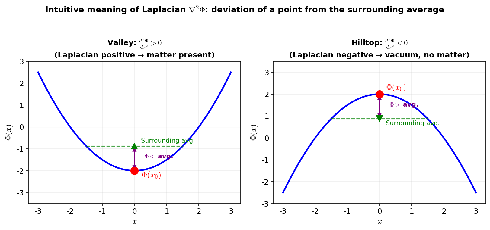
Fig. 1.8: Intuitive meaning of the Laplacian \(\nabla^2\Phi\). Left: at a valley bottom, \(\Phi\) is less than the surrounding average → \(d^2\Phi/dx^2 > 0\) (positive Laplacian). Right: at a hilltop, \(\Phi\) is greater than the surrounding average → \(d^2\Phi/dx^2 < 0\) (negative Laplacian). The Poisson equation expresses that "valleys form where matter exists."
🔵 Kai: Hmm... in one dimension I understand that "valley bottom means positive second derivative," but in three dimensions the idea that "the \(r\)-direction curvature and angular directions cancel" is honestly still fuzzy. But as a bottom line, it's "the Laplacian is positive—meaning there's a valley—where matter exists"?
🟡 Lina: That's right. At this stage, it's sufficient to just hold onto the conclusion: "\(\nabla^2\Phi = 0\) where there's no matter, \(\nabla^2\Phi > 0\) where there is matter." If you're curious about how the cancellation works, let me give just one concrete image. When there's mass at the origin, surround a point \(P\) with a small sphere. If \(P\) is outside the origin, there's no mass inside that small sphere. \(\Phi\) is deeper on the "Sun-side" of the sphere and shallower on the "opposite side"—it's asymmetric, but the average exactly matches the value at \(P\). "Matching the average = no deviation from surroundings = Laplacian is zero." On the other hand, if \(P\) is at the origin (where the mass is), \(\Phi\) is higher in the surroundings than at \(P\)—the average exceeds the value at \(P\)—so the Laplacian is positive. The rigorous calculation is deferred to General Relativity Ch. 1, but remember the image of "comparing with the surrounding average."
🔵 Kai: I get the "judge by whether it matches the average" idea. But why does it exactly match the average outside the origin? If the Sun-side is deeper and the opposite side is shallower, it seems like the average should deviate a bit from the value at \(P\)...
🟡 Lina: Good question. Intuitively, the "Sun-side" of the sphere is deeper than \(P\) but covers a smaller area, while the "opposite side" is shallower but covers a larger area—this asymmetry exactly cancels out. It's a special property of the \(1/r\) function. For a general function, this wouldn't happen. The rigorous proof using Gauss's law is in General Relativity Ch. 1, so for now remember that "it's precisely because \(\Phi = -GM/r\) has this special form that the Laplacian is zero away from the origin."
🔵 Kai: I see, it's a special property of \(1/r\). I'll accept just the conclusion for now.
🟡 Lina: Right. Where matter exists, \(\rho > 0\) so \(\nabla^2\Phi > 0\), meaning the potential forms a "valley" that's lower than the surroundings. Objects fall toward that valley—this is the true nature of gravity.
🔵 Kai: Does the \(\Phi = -GM/r\) from earlier satisfy this equation?
🟡 Lina: Good question. When mass \(M\) is concentrated at a single point (the origin), \(\rho = 0\) everywhere except the origin, so \(\nabla^2 \Phi = 0\) must be satisfied there. Indeed, \(\Phi = -GM/r\) satisfies this away from the origin. The rigorous verification and derivation—including explanations of gradient, partial derivatives, and the procedure of deriving the Poisson equation from Gauss's divergence theorem—are carefully treated in General Relativity Ch. 1, so please refer to that.
🔵 Kai: I see. So to summarize the physical meaning of the Poisson equation: "where matter exists, the curvature of the potential doesn't vanish—the more matter, the greater the curvature"?
🟡 Lina: Exactly.
🟡 Lina: One important note. The left side of the Poisson equation contains no time derivatives. This means that when the mass distribution \(\rho\) changes, the potential \(\Phi\) changes instantaneously throughout all of space. In other words, it implicitly assumes that changes in gravity propagate at infinite speed. This will later turn out to contradict special relativity (Ch. 5)—it's one of the reasons general relativity becomes necessary in Ch. 6.
🔵 Kai: Propagating instantaneously... does that mean faster than light? It didn't seem to be a problem with Neptune earlier.
🟡 Lina: And this "field" way of thinking will appear repeatedly in electromagnetism (Ch. 2) and general relativity (Ch. 6). By rewriting Newton's model in the language of fields, the connections to later chapters become easier to see.
⚪ Mei: So that's why you said "we'll need this in later chapters" at the beginning.
📝 Exercises:
- Derive the gravitational potential from the Poisson equation → Problem M-2. Calculation of the Gravitational Potential
✅ Comprehension Check: What does the Poisson equation \(\nabla^2 \Phi = 4\pi G \rho\) represent?
Answer
It represents that curvature arises in the gravitational potential where matter (mass density \(\rho\)) exists. It's the relation that determines the potential from the mass distribution. Because it contains no time derivatives, it implicitly assumes that changes in gravity propagate instantaneously.
1.7 Another Formulation — The Principle of Least Action
🟡 Lina: Let me introduce another formulation of Newtonian mechanics here. This will appear repeatedly in Ch. 8 on quantum field theory and Ch. 13 on string theory—it's one of the most important principles in all of physics.
🟡 Lina: Newton's \(F = ma\) is a causal description saying "force determines acceleration." But the same physics can be described from a completely different perspective. The principle of least action.
🔵 Kai: What's "least action"?
🟡 Lina: First, let me define the Lagrangian \(L\). With kinetic energy \(T\) and potential energy \(V\),
🔵 Kai: \(T - V\) and not \(T + V\)? Why subtraction?
🟡 Lina: Good question. For now, accept that "defining it as \(T - V\) produces the correct equations of motion." The reason will become natural when you learn the calculus of variations in General Relativity Ch. 1.
🟡 Lina: Next, define the action \(S\). It's the Lagrangian \(L\) integrated over time from \(t_1\) to \(t_2\):
This is "the total of \(L\)'s values at each instant, added up from departure to arrival." It's the same operation as computing a definite integral in high school—imagine drawing a graph with time on the horizontal axis and the value of \(L\) on the vertical axis, then finding the signed area. Let me use the word "path" here. Suppose an object is at position \(q_1\) at time \(t_1\) and at position \(q_2\) at time \(t_2\). There are infinitely many possible ways it could move in between—what speed it travels at along the way. Each such way of moving is called a "path."
🔵 Kai: "Different paths" means, for example, there are various patterns of accelerating or decelerating along the way while connecting the same start and end points?
🟡 Lina: Exactly. Since \(L = T - V\), different paths mean different velocities and positions at each moment, so \(T\) and \(V\) change. As a result, the time evolution of \(L\) changes, and the value of the action \(S\) changes. The principle of least action claims that "among all possible paths, the path that makes this action \(S\) a stationary value is the physically realized path."
🔵 Kai: What's a "stationary value"? Is it different from a minimum?
🟡 Lina: A stationary value means that when you change the path by just a tiny amount, \(S\) barely changes. It's the same idea as "derivative = 0 is the condition for an extremum" that you learned in high school—at the bottom of the parabola \(y = x^2\) (\(x = 0\)), shifting \(x\) slightly changes \(y\) proportionally to the square of the shift, so the first-order change is zero, right? The same applies to paths: "the first-order change in \(S\) when the path is changed slightly equals zero" is the condition for a stationary value. In most cases it's a minimum, which is why it's called the "principle of least action," but strictly speaking it's not always a minimum—like a mountain pass, which is the highest point in the east-west direction but the lowest in the north-south direction, right? Such a "stationary point that's neither a minimum nor maximum" is a saddle point. But at this stage, think of it as "roughly a minimum" (Fig. 1.9 "Principle of least action and path comparison").
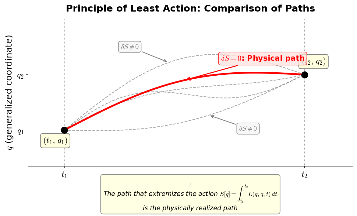
Fig. 1.9: Principle of least action and path comparison. Among various paths from start \((t_1, q_1)\) to end \((t_2, q_2)\), the path that extremizes the action \(S\) (solid line) is the physically realized path.
⚪ Mei: Instead of "considering forces at each instant," it's the idea of "surveying the entire path and selecting the optimal one."
🟡 Lina: In Fig. 1.10 "Visualization of the action integral", let's see how \(L(t)\) changes for different paths and how the action \(S\) (area) changes.
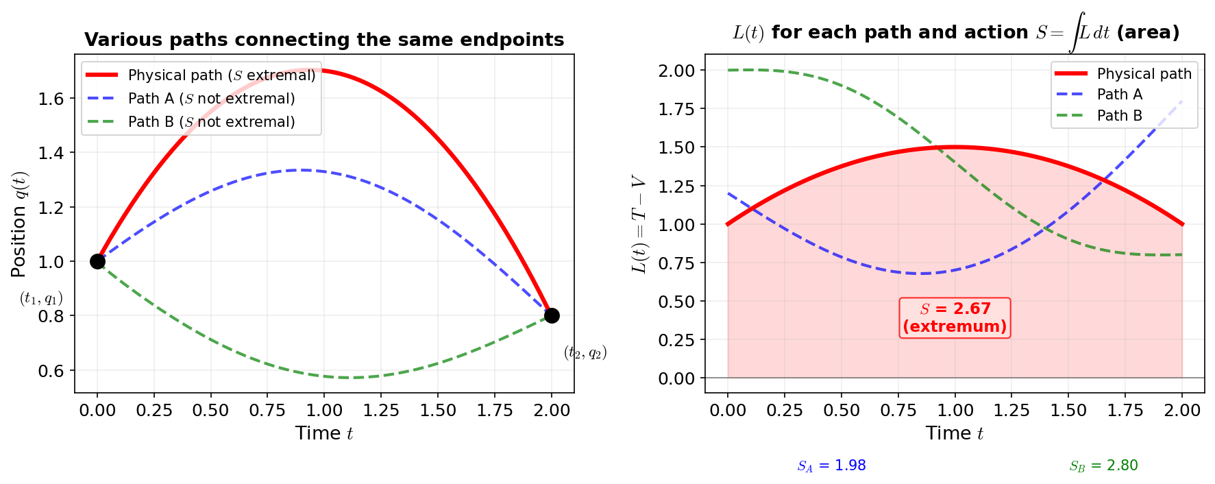
Fig. 1.10: Visualization of the action integral. Left: various paths connecting the same start and end points. Right: graphs of \(L(t)\) for each path. The area between the curve and horizontal axis corresponds to the action \(S = \int L\,dt\). The physical path (red solid line) is the path for which \(S\) is extremized.
🟡 Lina: From this principle, an equation that the realized path must satisfy can be derived. That's the Euler-Lagrange equation:
Some unfamiliar symbols appeared. Don't worry—I'll explain each one. First, \(q\) is a symbol representing the object's position—the same thing as the \(x\) we've been using. In physics there's a convention of writing position generally as \(q\) (called a "generalized coordinate"). \(\dot{q}\) is the time derivative of \(q\), \(dq/dt\)—that is, velocity. Physics often uses this dot notation.
🔵 Kai: So the dot represents a time derivative. \(\dot{q}\) is velocity and \(\ddot{q}\) is acceleration.
🟡 Lina: Exactly. Next, the meaning of \(\partial\) (the rounded d). Since \(L\) depends on both \(q\) and \(\dot{q}\), we need to consider "the rate of change when only one of them is varied." \(\partial L / \partial \dot{q}\) is called a partial derivative, meaning "the rate of change of \(L\) when only \(\dot{q}\) is varied while holding \(q\) fixed." While the ordinary derivative \(d/dt\) tracks "everything changing with time," the partial derivative is the operation of "freezing other variables and moving just one." For a simple example, given a two-variable function \(f(x, y) = x^2 + 3y\), \(\partial f/\partial x\) means "treat \(y\) as a constant and differentiate with respect to \(x\)," giving \(2x\). \(\partial f/\partial y\) means "treat \(x\) as a constant and differentiate with respect to \(y\)," giving \(3\). What you're doing is the same as ordinary differentiation—you just "treat the variables you're not moving as constants." The detailed treatment of partial derivatives is in General Relativity Ch. 1.
🔵 Kai: The symbols are overwhelming, but... does this really give \(F = ma\)? Especially \(\frac{\partial L}{\partial \dot{q}}\)—differentiating \(L\) with respect to velocity. \(L\) contains both position and velocity, so how do you differentiate with respect to just one?
🟡 Lina: Good question. Let me add one supplement: the Euler-Lagrange equation is the mathematical translation of the condition "the action \(S\) doesn't change when the path is shifted by a tiny amount." The specific calculation of that translation (calculus of variations) is done carefully in General Relativity Ch. 1, but let's verify now that just using the result gives \(F = ma\). The symbols look numerous, but if you substitute step by step, it'll be fine. Specifically, let's consider one-dimensional motion with \(q = x\) (position). Let's substitute \(L = \frac{1}{2}m\dot{x}^2 - V(x)\).
🔵 Kai: Okay. So where do I start?
🟡 Lina: Start with the first term of the Euler-Lagrange equation, \(\frac{d}{dt}\frac{\partial L}{\partial \dot{x}}\). To find \(\partial L / \partial \dot{x}\), we view it as a function of \(\dot{x}\) only with \(x\) held fixed—this is exactly the "differentiate with respect to just one" that Kai asked about. \(V(x)\) doesn't contain \(\dot{x}\), so taking the partial derivative with respect to \(\dot{x}\) gives zero and it vanishes. What remains is just \(\frac{1}{2}m\dot{x}^2\). If you think of \(\dot{x}\) as a single variable \(u\), it's the same as differentiating \(\frac{1}{2}mu^2\) with respect to \(u\)—\(\frac{d}{du}\left(\frac{1}{2}mu^2\right) = \frac{1}{2}m \cdot 2u = mu\), so \(\frac{\partial}{\partial \dot{x}}\left(\frac{1}{2}m\dot{x}^2\right) = m\dot{x}\).
⚪ Mei: So \(\frac{\partial L}{\partial \dot{x}} = m\dot{x}\). That's the same form as momentum \(p = mv\).
🔵 Kai: Ah, even though it's called a partial derivative, what you're actually doing is just "treating everything except \(\dot{x}\) as a constant and differentiating normally." It's less scary than I thought.
🟡 Lina: Exactly. Since \(m\) is a constant, differentiating this with respect to time gives \(\frac{d}{dt}(m\dot{x}) = m\ddot{x}\) (two dots means the second time derivative, i.e., acceleration). Next, find the second term, \(\frac{\partial L}{\partial x}\). This time hold \(\dot{x}\) fixed and view it as a function of \(x\) only. \(\frac{1}{2}m\dot{x}^2\) doesn't contain \(x\), so it vanishes, and what remains is the partial derivative of \(-V(x)\) with respect to \(x\). Since \(V\) is a function of \(x\) alone, the partial derivative gives the same result as the ordinary derivative: \(\partial L / \partial x = -dV/dx\).
🔵 Kai: Ah, so the first term becomes acceleration and the second becomes something related to force.
🟡 Lina: Right! Putting them into the Euler-Lagrange equation:
The right side \(-dV/dx\) represents "force acts in the direction where potential energy drops steeply"—this is the force \(F\) itself—the same as "conservative force equals minus the slope of potential energy" that you learned in high school. So this is \(F = ma\).
🔵 Kai: Wow, \(F = ma\) really came out! It looked like a detour, but we arrived at the same place.
🟡 Lina: The full steps of deriving the Euler-Lagrange equation from the calculus of variations—the variation calculation, integration by parts, and vanishing of boundary terms—are treated in detail in General Relativity Ch. 1, so refer to that. For now, it's enough to grasp that "once you specify the Lagrangian, the equations of motion come out automatically."
📝 Exercises:
- Check how the results change with \(T-V\) versus \(T+V\) → Problem B-2. Why T-V and Not T+V
🔵 Kai: If the same answer comes out, what's the point of having a different formulation?
🟡 Lina: There are three reasons. First, symmetries become visible—it directly connects to the powerful theorem that "symmetries produce conserved quantities" (Noether's theorem). I'll explain this shortly.
🔵 Kai: Conserved quantities from symmetries...? I don't quite get it yet, but I think concrete examples will help.
🟡 Lina: Second, it's coordinate-independent—whether in Cartesian or polar coordinates, the same Lagrangian produces the correct equations. In general relativity (Ch. 6), coordinate-independent description becomes essentially important. Third, extension to field theory and string theory is natural—in Ch. 8 on quantum field theory we start from "the field Lagrangian," and in Ch. 13 on string theory it's used directly in the form "minimize the action of the string (the area of the worldsheet)."
⚪ Mei: So \(F = ma\) is language exclusive to Newtonian mechanics, but "specify a Lagrangian and extremize the action" is a common language that works in electromagnetism, quantum field theory, and string theory alike.
What Is Symmetry — "Unchanged Under a Change"
In physics, "having a symmetry" means the laws of physics don't change under a certain operation.
Operation Name of symmetry Resulting conserved quantity Shift the location of an experiment Spatial translation symmetry Momentum Shift the time of an experiment Time translation symmetry Energy Rotate the experimental apparatus Rotational symmetry Angular momentum "For every symmetry, one conserved quantity emerges"—this is Noether's theorem (treated in detail in Quantum Field Theory Quantum Field Theory Ch. 3). The more symmetries a system has, the more constrained its behavior, and the easier the calculations become.
In Ch. 9, more abstract symmetries (gauge symmetries) appear. From the symmetry "physics doesn't change when we change the phase of the wave function," the electromagnetic force is automatically derived. For now, it's enough to remember "symmetry = physics doesn't change under a certain operation."
Note: Symmetries are not "things nature must necessarily possess." They are verified as part of a hypothesis in the form "if we assume this symmetry, results consistent with experiment emerge." In fact, in Ch. 9, symmetries can even be "spontaneously broken" (the Higgs mechanism)—the subtle situation where the Lagrangian has the symmetry but the realized state does not. Physicists tend to find theories with symmetry "beautiful" and prefer them. The more symmetries, the more constrained the calculations and the greater the predictive power. However, "beautiful" doesn't necessarily mean "correct"—this point will be questioned again in Ch. 22 (criticisms of string theory).
✅ Comprehension Check: What does Noether's theorem claim? Give one specific example.
Answer
It claims that for every symmetry, one conserved quantity emerges. For example, time translation symmetry (physics doesn't change when you shift the time of an experiment) leads to energy conservation.
🟡 Lina: Let me summarize the differences between the two formulations in a table.
Table 1.2: Comparison of the Newtonian formulation and the Lagrangian formulation
| Newtonian formulation | Lagrangian formulation | |
|---|---|---|
| Fundamental equation | \(F = ma\) | \(\frac{d}{dt}\frac{\partial L}{\partial \dot{q}} - \frac{\partial L}{\partial q} = 0\) |
| Starting point | Specify force (a vector) | Specify Lagrangian \(L = T - V\) (a scalar) |
| Perspective | Cause and effect at each instant | Surveying the entire path |
| Coordinate system | Cartesian coordinates are basic | Same form in any coordinate system |
| Symmetry → conserved quantity | Must be checked individually | Automatic via Noether's theorem |
| Extensibility | Mechanics only | Common to electromagnetism, field theory, string theory |
🔵 Kai: So with \(F = ma\) you can only use it in Newtonian mechanics, but with the principle of least action you can use it directly in other fields too? But if the form of the Lagrangian differs by field, doesn't it end up being a different story for each one?
🟡 Lina: Good question. Even though the forms differ, the framework of "write a Lagrangian, extremize the action → equations of motion come out" is common to all. All fundamental models in physics can be formulated using this same procedure. This is the tool we'll keep using from here on.
🔵 Kai: Ah, so the contents differ but the "recipe procedure" is the same. But where does the guarantee come from that this recipe is correct? It might just be that it's worked by coincidence so far, right?
🟡 Lina: Sharp observation. There is no guarantee. There's only the empirical fact that "models writable via the principle of least action have, so far, all agreed with experiment." If a model that doesn't agree is found, we'd need to revisit the framework itself. But so far, from particle physics to cosmology, all fundamental models can be written in this form.
⚪ Mei: In other words, \(F = ma\) is language specific to Newtonian mechanics, but "specify a Lagrangian and extremize the action" is a common language that works across electromagnetism, quantum field theory, and string theory.
🟡 Lina: And what's important is that the Lagrangian itself is a "hypothesis." The job of physicists is "to find the correct Lagrangian." In Newtonian mechanics it's \(L = T - V\), in electromagnetism it takes a different form (Ch. 2), in string theory yet another form (Ch. 13)—the contents of the Lagrangian differ by field, but "find it and extremize the action" is the common methodology of physics.
⚪ Mei: So what was said in the Prologue about "models are hypotheses" concretely means "which Lagrangian to choose is the hypothesis."
🔵 Kai: ...So if it doesn't match experiment, you rewrite the Lagrangian?
🟡 Lina: Exactly. When phenomena are found that the Newtonian mechanics Lagrangian can't explain, we search for a new Lagrangian. That's how physics progresses. The "limits of Newton's model" we'll see at the end of this chapter lead precisely to that kind of story.
✅ Comprehension Check: State the definition of the Lagrangian \(L\) and the definition of the action \(S\).
Answer
The Lagrangian is \(L = T - V\) (kinetic energy minus potential energy). The action is \(S = \int_{t_1}^{t_2} L\,dt\) (the Lagrangian integrated over time). The principle of least action claims that the physically realized path is the one that extremizes \(S\).
✅ Comprehension Check: Give one reason why the principle of least action is superior to \(F = ma\).
Answer
(Any one of the following) (1) The relationship between symmetries and conserved quantities becomes automatically visible. (2) It's coordinate-independent. (3) Extension to field theory and string theory is natural.
1.8 What Newton's Model Cannot Explain — Foreshadowing
🟡 Lina: Now, Newton's model was astonishingly successful. Planetary orbits, tides, ballistic trajectories, Neptune's position—all explained from a single equation. But there are things it cannot explain.
🔵 Kai: Like what?
🟡 Lina: Three major ones.
First Limitation: It Doesn't Explain "Why Things Attract"
🟡 Lina: \(F = GMm/r^2\) tells us "how the magnitude of the force is determined," but it says absolutely nothing about "why objects with mass attract each other." Newton himself acknowledged this, stating "I frame no hypotheses (Hypotheses non fingo)."
⚪ Mei: So Newton's model answered the "why" of Kepler's laws, but for the "why" of universal gravitation itself, an even deeper model is needed.
Second Limitation: Gravity Propagates Instantaneously
🟡 Lina: As we confirmed in 1.6 "Gravitational Potential and the Poisson Equation", the Poisson equation \(\nabla^2\Phi = 4\pi G\rho\) contains no time derivatives. This means changes in gravity propagate instantaneously. Concretely, if the Sun suddenly vanished, in Newton's model the Earth would instantaneously begin moving in a straight line. Even though light takes about 8 minutes to travel from the Sun to Earth.
🔵 Kai: Doesn't that mean information travels faster than light?
🟡 Lina: Yes. Compare the difference between the two models in Fig. 1.11 "Contrast between Newton's model (left) and the requirement of special relativity (right)".
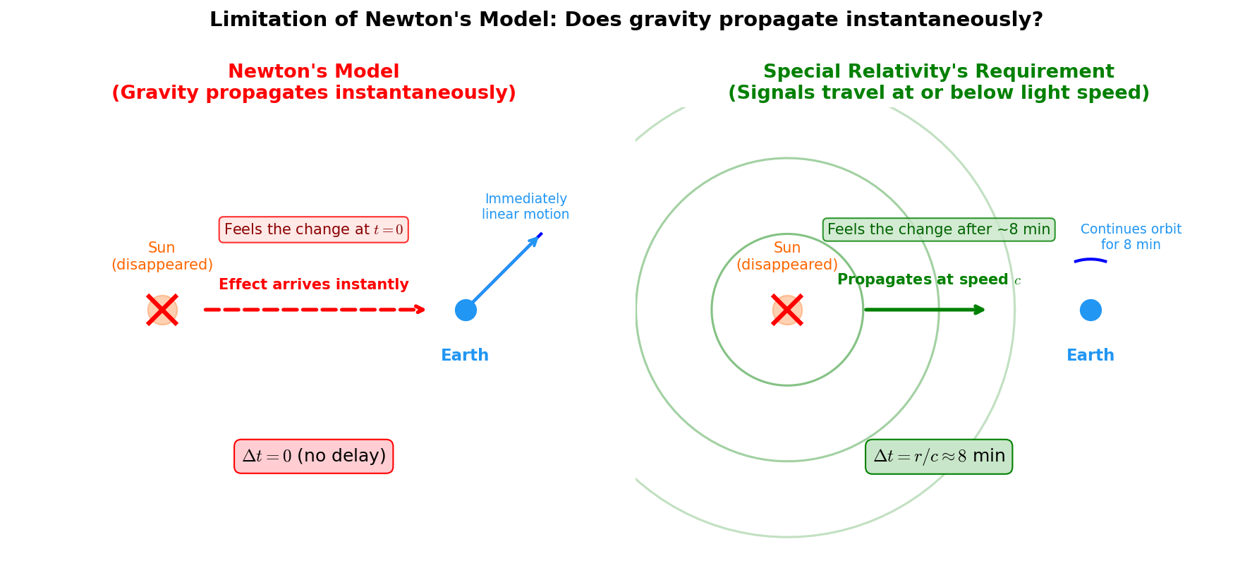
Fig. 1.11: Contrast between Newton's model (left) and the requirement of special relativity (right). In Newton's model, Earth is affected the instant the Sun disappears, but in relativity, information can only travel at or below the speed of light \(c\), so there is a delay of about 8 minutes.
🟡 Lina: The principle of Einstein's special relativity (Ch. 5)—"no signal can travel faster than the speed of light"—is incompatible with Newtonian gravity.
Third Limitation: Mercury's Perihelion Precession
🟡 Lina: Mercury's orbit is an ellipse, but that ellipse slowly rotates (the perihelion shifts). Look at Fig. 1.12 "Mercury's perihelion precession". After subtracting all influences from other planets, an "unexplainable" discrepancy of about 43 arcseconds per century remains. Newton's model cannot explain this.
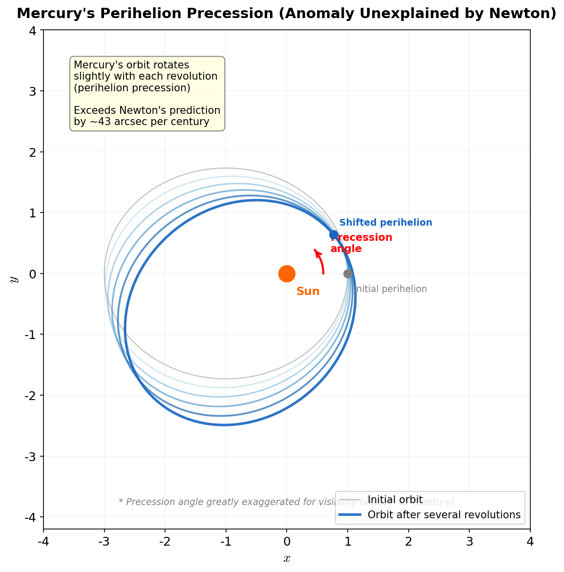
Fig. 1.12: Mercury's perihelion precession. With each orbit, the elliptical orbit rotates slightly, shifting the perihelion position. Even after accounting for all other planetary influences, Newton's model cannot explain the excess of about 43 arcseconds per century (angles greatly exaggerated in the figure).
🔵 Kai: With Neptune, it was solved by "there's an unknown planet," but that didn't work this time?
⚪ Mei: In other words, Newton's model is an "approximation," and a more accurate model is needed.
🟡 Lina: Exactly. That "more accurate model" is general relativity (Ch. 6). But that's a story for later. For now, it's enough to understand how successful Newton's model was and where its limitations lie. I've summarized the big picture of this chapter in Fig. 1.13 "Achievements and limitations of Newtonian gravity". We'll revisit Mercury's perihelion precession in Ch. 4.
%%{init: {"theme": "default", "themeCSS": ".edgePath .path, .flowchart-link { stroke-width: 2px !important; }"}}%%
flowchart TD
    N["Newton's Universal Gravitation<br>F = GMm/r²"] --> K["Derives Kepler's 3 Laws"]
    N --> C["Newton's Cannonball<br>Unification of terrestrial and celestial"]
    N --> NP["Discovery of Neptune<br>Quantitative prediction"]
    N --> L1["❌ Why do things attract?<br>No explanation"]
    N --> L2["❌ Gravity propagates instantaneously<br>Contradicts special relativity"]
    N --> L3["❌ Mercury's perihelion precession<br>43 arcsec/century"]
    L1 --> GR["General Relativity<br>(Chapter 6)"]
    L2 --> GR
    L3 --> GR
    style N fill:#2196F3,color:#fff
    style GR fill:#FF9800,color:#fff
    style L1 fill:#ffcdd2
    style L2 fill:#ffcdd2
    style L3 fill:#ffcdd2
    style K fill:#c8e6c9
    style C fill:#c8e6c9
    style NP fill:#c8e6c9
Fig. 1.13: Achievements and limitations of Newtonian gravity
✅ Comprehension Check: List two or more limitations that Newton's model cannot explain.
Answer
(1) It doesn't explain "why objects with mass attract each other." (2) Gravity propagates instantaneously, allowing information transfer faster than light (contradicting special relativity). (3) It cannot explain Mercury's perihelion precession (43 arcseconds/century).
Preview of Next Chapter
Ch. 2 — Just as Newton unified "the terrestrial and celestial" with gravity, Faraday and Maxwell unified electricity and magnetism into a single model. And the "speed of light" predicted by that model becomes the key to breaking through the limitations of Newtonian gravity.
References
The content of this chapter was constructed with reference to the following works.
- David Tong, Lectures on General Relativity, Ch.1: "Geodesics in Spacetime" — Formulation of Newtonian mechanics as a field theory, contradiction with special relativity
- Carlo Rovelli, Reality Is Not What It Seems, Ch.2: "The Classics" — Historical context from Pythagoras to Newton
- Barton Zwiebach, A First Course in String Theory, Ch.3: "Electromagnetism and gravitation in various dimensions" — Dimensional dependence of gravity
- David Tong, Lectures on General Relativity, Ch.2: "Introducing Differential Geometry" — Principle of least action, introduction of the Lagrangian, source material for exercises
- David Tong, Lectures on Quantum Field Theory, Ch.2: "Free Fields" — Noether's theorem, relationship between symmetries and conserved quantities
- Barton Zwiebach, A First Course in String Theory, Ch.8: "World-sheet currents" — Concrete calculations deriving conserved quantities from symmetries
- 須藤靖『解析力学・量子論』Ch.4 — Axiomatic introduction of the principle of least action, explanation that the Lagrangian is not limited to \(T - V\)
- 清水明『新版 量子論の基礎』Ch.4, Ch.7 — Lagrangians for finite degrees of freedom and fields, principle of least action
Feedback on this page
Let us know if something was unclear, incorrect, or could be improved.