Chapter 2: Can Electricity and Magnetism Be Unified? — The Birth of Electromagnetism
Story so far: In Ch. 1, we saw how Newton could explain planetary orbits, tides, and cannonball trajectories from a single model of universal gravitation. The discovery of Neptune dramatically demonstrated the power of quantitative prediction through equations. However, Newton's model left behind problems: it could not explain "why things attract" and assumed "gravity propagates instantaneously." In this chapter, we look at another unification story that took place in a different domain from Newton's — electricity and magnetism.
Goals of This Chapter
- Experience the power of unification: "phenomena that appear separate can actually be described by a single model"
- Follow the story of how Maxwell unified electricity and magnetism into 4 equations, and as a byproduct derived the prediction that "light is an electromagnetic wave"
- Furthermore, learn about electromagnetic potentials and gauge transformations, and confirm that unification gives rise to a new mystery — the invariance of the speed of light
2.1 Motivation: Are Electricity and Magnetism Separate Phenomena?
🟡 Lina: In Ch. 1, we talked about how Newton built a model of gravity. Today we're in a different domain — electricity and magnetism.
🔵 Kai: In high school, we learn them separately, right? Coulomb's law for static electricity, and then magnetism.
🟡 Lina: That's right. Until the 18th century, electricity and magnetism were considered completely separate phenomena. Electricity was what happened when you rubbed amber, and magnetism was a property of lodestone. Nobody thought they were related.
🔵 Kai: When did people figure out that electricity and magnetism are related?
🟡 Lina: In 1820, Ørsted discovered that "a compass needle moves near an electric current." This showed that electricity generates magnetism. And the reverse — magnetism generating electricity — was discovered by Faraday. That was the discovery of electromagnetic induction in 1831. When you move a magnet inside a coil, current flows.
⚪ Mei: So both directions — electricity→magnetism and magnetism→electricity — were confirmed experimentally.
🔵 Kai: That's the principle behind motors and generators, right?
🟡 Lina: Exactly. Up to this point, these were experimental facts. But the person who explained why electricity generates magnetism and magnetism generates electricity within a single unified model was Maxwell.
⚪ Mei: This has the same structure as Newton unifying "the falling apple" and "the Moon's orbit" in Ch. 1.
🔵 Kai: With Newton, Neptune was predicted, right? Does Maxwell's unification also produce some prediction?
🟡 Lina: That's exactly what we're going to see. Maxwell's unification produces a prediction just as dramatic as Newton's — in some sense, even more so. I've summarized this historical progression in a timeline (Fig. 2.1 "Historical timeline of the unification of electromagnetism").
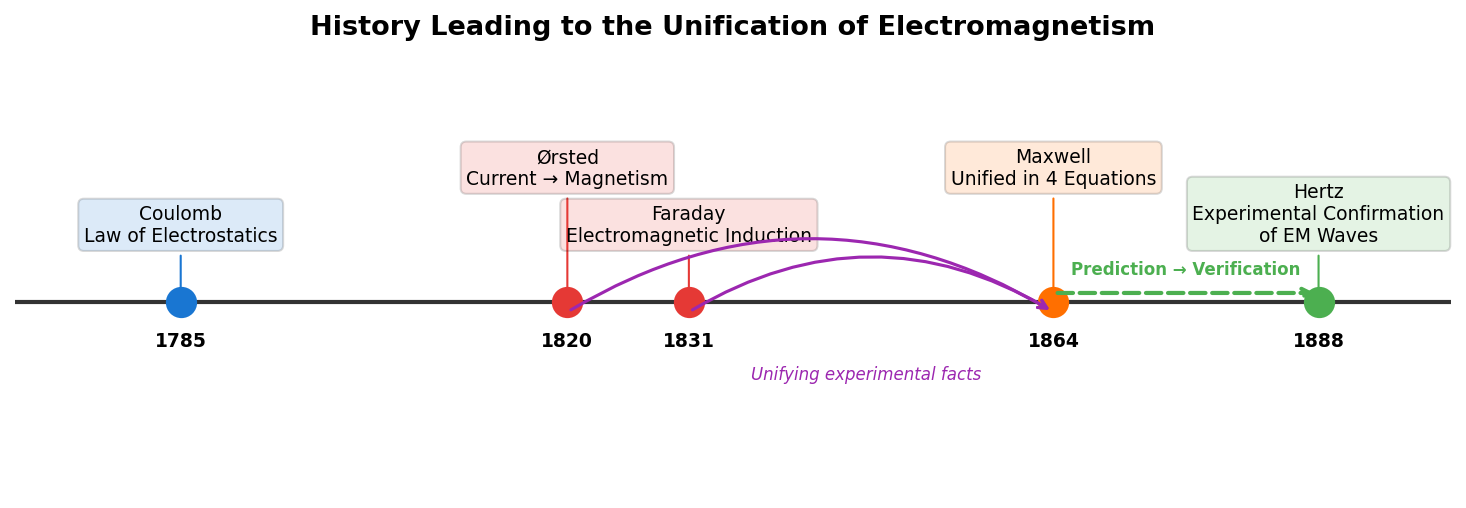
Fig. 2.1: Historical timeline of the unification of electromagnetism. From Coulomb's electrostatic law (1785) to Hertz's experimental confirmation of electromagnetic waves (1888), showing the accumulation of experimental facts, Maxwell's theoretical unification, and the verification of predictions.
✅ Comprehension Check: What phenomenon did Ørsted discover in 1820?
Answer
A compass needle moves near an electric current (electricity generates magnetism).
✅ Comprehension Check: What is the phenomenon of "electromagnetic induction" that Faraday discovered in 1831?
Answer
The phenomenon where current flows when a magnet is moved inside a coil. Magnetism generates electricity.
2.2 Faraday's Idea of the "Field"
🟡 Lina: To understand Maxwell's work, you first need to know about Faraday's idea.
🔵 Kai: What kind of person was Faraday?
🟡 Lina: He had no formal university education — he was a bookbinder's apprentice who became a scientist through self-study. But he was an experimental genius. And he created a concept that changed the history of physics: the idea of a field.
🔵 Kai: Field? That came up in Ch. 1 with gravitational potential, right?
🟡 Lina: Yes. In Newton's gravity, "distant objects directly pull on each other" — action at a distance. But Faraday had a different view. "A field of force extends through space itself, and objects experience force through that field." This is called local action.
🔵 Kai: We did an experiment in high school where you sprinkle iron filings around a magnet and patterns appear. Is that what a "field" means?
🟡 Lina: Yes, that's exactly the intuitive image of Faraday's "field." Faraday couldn't write equations, but he introduced the concept of the "field." And the person who formulated that concept mathematically was Maxwell. This relay between the two is one of the most beautiful in the history of physics. I've summarized the difference between action at a distance and local action in a figure (Fig. 2.2 "Comparison of action at a distance and local action").
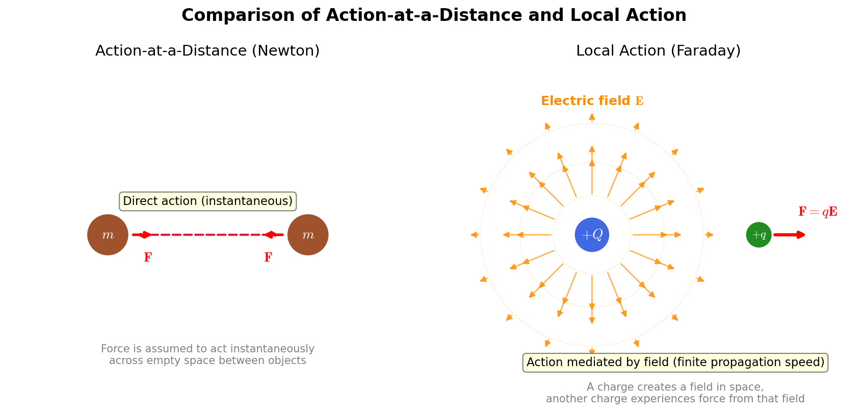
Fig. 2.2: Comparison of action at a distance and local action. In Newton's action at a distance (left), objects directly attract each other. In Faraday's local action (right), a field extends through space and objects experience force through the field.
🔵 Kai: So the gravitational potential \(\Phi(\mathbf{r})\) from Ch. 1 was a type of "field" too.
🟡 Lina: Yes. The gravitational potential is a scalar field that assigns a single number to each point. In electromagnetism, fields that assign a vector to each point appear. Let's organize this in the next section.
✅ Comprehension Check: What is the idea of the "field" that Faraday introduced?
Answer
The idea that a field of force extends through space itself, and objects experience force through that field (local action).
✅ Comprehension Check: Who formulated Faraday's concept of the "field" mathematically?
Answer
Maxwell.
2.3 Scalar Fields and Vector Fields
🟡 Lina: Before we get to Maxwell's equations, let me explain an important distinction. In Ch. 1, we introduced the gravitational potential \(\Phi(x,y,z)\), right? That was a function assigning a single number to each point — a scalar field.
🔵 Kai: It was like a temperature distribution map, right?
🟡 Lina: Yes. But the electric field \(\mathbf{E}\) is different. It assigns an arrow with direction and magnitude (a vector) to each point — a vector field. The magnetic field \(\mathbf{B}\) is the same.
🔵 Kai: I learned about vectors in high school. Force, velocity, things like that. But the electric field is invisible — how do you confirm it has a "direction"?
🟡 Lina: Good question. Place a small positive test charge at that point, and the direction and magnitude of the force the charge experiences — that's the direction and magnitude of the electric field. The electric field \(\mathbf{E}\) is a vector with 3 components \((E_x, E_y, E_z)\). In this book, vectors are written in boldface (\(\mathbf{E}\)). Scalars (ordinary numbers) are in regular typeface (\(\Phi\)).
⚪ Mei: To summarize:
| Type | What's assigned to each point | Examples |
|---|---|---|
| Scalar field | A single number | Temperature \(T(\mathbf{r})\), gravitational potential \(\Phi(\mathbf{r})\) |
| Vector field | A vector (direction + magnitude) | Electric field \(\mathbf{E}(\mathbf{r})\), magnetic field \(\mathbf{B}(\mathbf{r})\) |
Table 2.1: Comparison of scalar fields and vector fields
🔵 Kai: Gravitational potential is a scalar field, and the electric and magnetic fields are vector fields — they differ in the number of components.
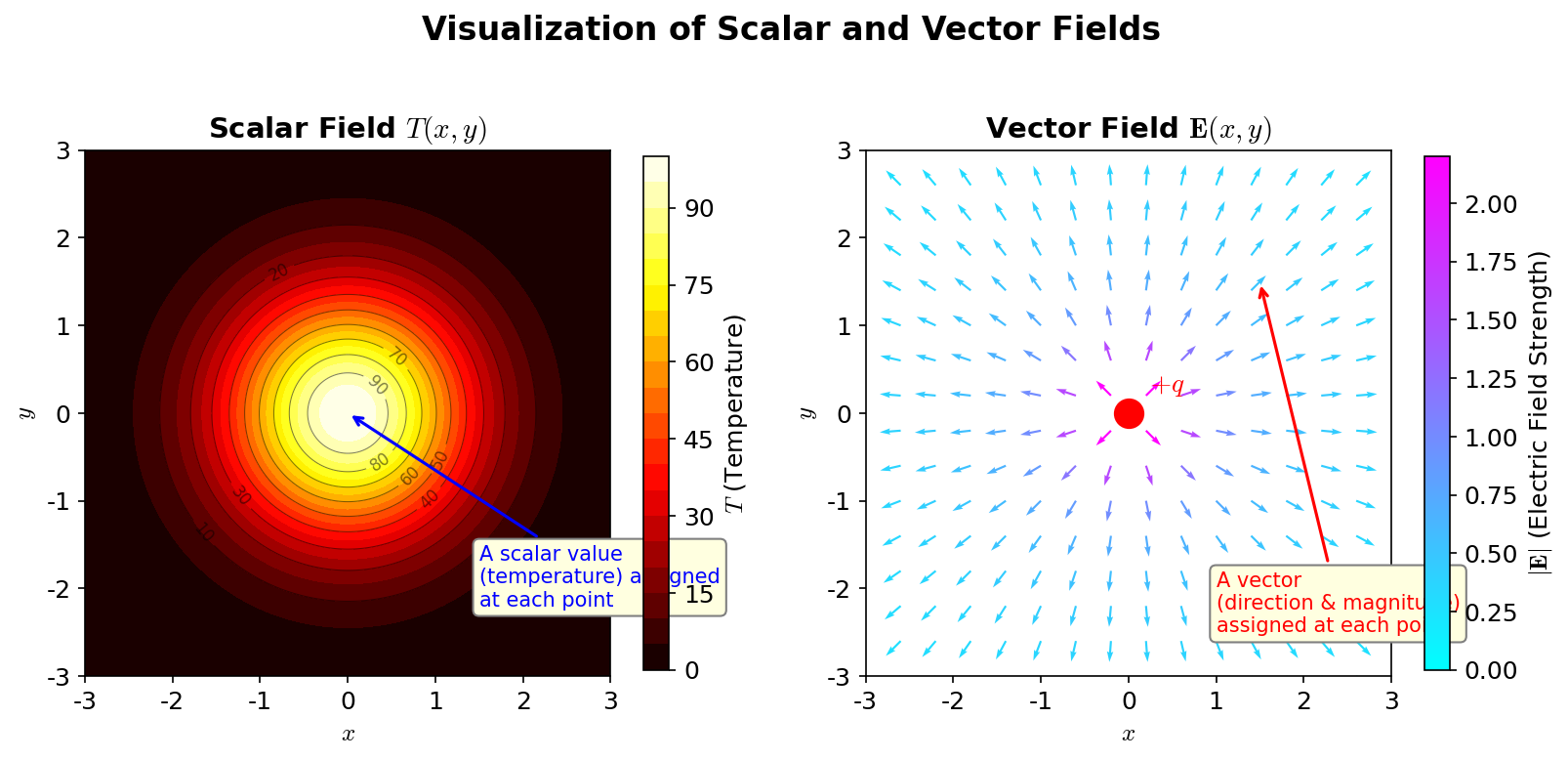
Fig. 2.3: Visualization of scalar and vector fields. Left: A scalar field (assigning a number to each point, displayed with contour lines). Right: A vector field (assigning an arrow to each point).
🟡 Lina: Looking at Fig. 2.3 "Visualization of scalar and vector fields", you can see that the scalar field is represented with contour lines and the vector field with arrows. The definitions of the differential operators we'll use — \(\nabla\) (nabla), \(\nabla \cdot\) (divergence), \(\nabla \times\) (curl) — are summarized in Appendix A, so refer to it as needed. \(\nabla\) is a vector operator representing "the direction and magnitude of spatial change," and in 3 dimensions it's written as \(\nabla = \left(\frac{\partial}{\partial x}, \frac{\partial}{\partial y}, \frac{\partial}{\partial z}\right)\). Let me just briefly state the physical meanings using this (also see Fig. 2.4 "Intuitive images of divergence and curl"):
- \(\nabla \cdot \mathbf{F}\) (divergence): The degree to which the vector field \(\mathbf{F}\) is "flowing outward" from that point
- \(\nabla \times \mathbf{F}\) (curl): The degree to which the vector field \(\mathbf{F}\) is "swirling" around that point
- \(\nabla^2 f\) (Laplacian): A quantity representing "how much the value at a point deviates from the average of its surroundings" for a scalar field \(f\) (it plays a central role in the wave equation in 2.5 "The Nature of Light — A Prediction from Maxwell's Equations"). Specifically, \(\nabla^2 f = \frac{\partial^2 f}{\partial x^2} + \frac{\partial^2 f}{\partial y^2} + \frac{\partial^2 f}{\partial z^2}\). For a vector field \(\mathbf{F}\), since each component \(F_x, F_y, F_z\) is an independent scalar field, we define \(\nabla^2 \mathbf{F} = (\nabla^2 F_x,\; \nabla^2 F_y,\; \nabla^2 F_z)\) by applying \(\nabla^2\) to each component separately (meaning we examine "how each direction of the field curves spatially" direction by direction)
🔵 Kai: "Outflow," "swirl," "deviation from the surrounding average" — they're all tools for describing changes in space.
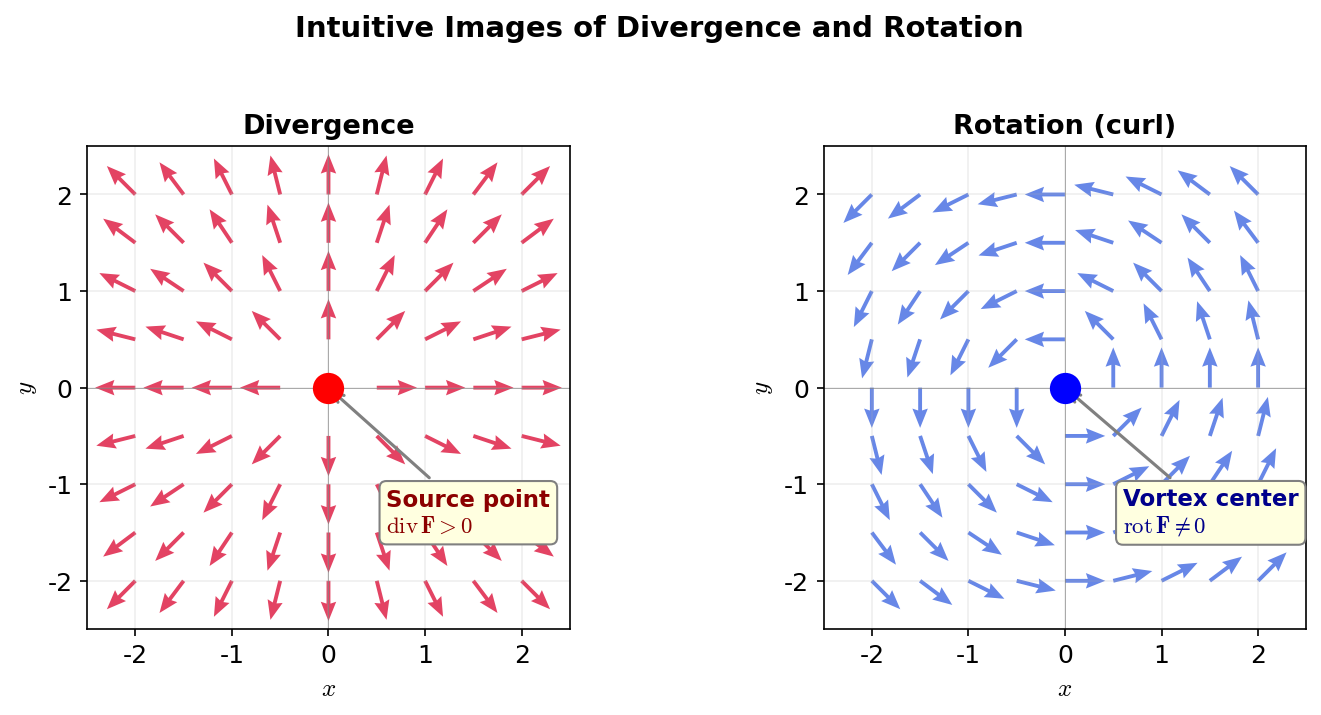
Fig. 2.4: Intuitive images of divergence and curl. Left: At a point where divergence (div) is positive, the field flows outward. Right: At a point where curl (rot) is nonzero, the field swirls.
✅ Comprehension Check: What is the difference between a scalar field and a vector field?
Answer
A scalar field is a function that assigns a single number to each point (e.g., gravitational potential \(\Phi\)). A vector field is a function that assigns a vector with direction and magnitude to each point (e.g., electric field \(\mathbf{E}\)).
2.4 Maxwell's Equations — The Unification of Electricity and Magnetism
🟡 Lina: In the 1860s, Maxwell summarized all experimental facts about electricity and magnetism into 4 equations.
🔵 Kai: Just 4?
🟡 Lina: Just 4. Let's look at each equation together with its meaning.
Equation 1: Gauss's Law
🟡 Lina: \(\rho\) (rho) is the charge density — how much charge exists at each point in space. \(\varepsilon_0\) (epsilon-zero) is the permittivity of free space — a constant representing the electrical property of vacuum. \(\nabla \cdot\) (nabla-dot) is the "divergence" (see Appendix A) — it tells you whether the vector field is flowing outward from that point.
🟡 Lina: So this equation says that electric field lines emerge from where there is charge \(\rho\). Outward from positive charges, inward toward negative charges.
✅ Comprehension Check: What does the first Maxwell equation (Gauss's law) \(\nabla \cdot \mathbf{E} = \rho/\varepsilon_0\) physically mean?
Answer
It means that electric field lines emerge from where there is charge. Field lines point outward from positive charges and inward toward negative charges.
Equation 2: Gauss's Law for Magnetism
🟡 Lina: \(\mathbf{B}\) is the magnetic field (magnetic flux density). It's also a vector field. The right side being zero means magnetic field lines have no "sources." In other words, there are no "magnetic monopoles" — no isolated N pole or S pole. Magnetic field lines always form closed loops.
🔵 Kai: When you break a magnet, you always get both an N pole and S pole together — that's what this equation is saying, right?
🟡 Lina: Yes. No matter how small you break it, you never get a monopole — that's the physical content of this equation.
Equation 3: Faraday's Law
🟡 Lina: \(\nabla \times\) (nabla-cross) is the "curl" (see Appendix A) — it tells you whether the vector field is swirling around that point. The right side \(\frac{\partial \mathbf{B}}{\partial t}\) represents "how the magnetic field at that point changes with time while holding position fixed" — it's the vector obtained by differentiating each component \(B_x, B_y, B_z\) with respect to time.
🟡 Lina: So, when the magnetic field \(\mathbf{B}\) changes in time, a curl in the electric field \(\mathbf{E}\) is generated. This is the mathematical expression of electromagnetic induction — the phenomenon Faraday discovered.
✅ Comprehension Check: Under what conditions does the third Maxwell equation (Faraday's law) state that a curl in the electric field arises?
Answer
A curl in the electric field \(\mathbf{E}\) arises when the magnetic field \(\mathbf{B}\) changes in time. This is the mathematical expression of electromagnetic induction discovered by Faraday.
Equation 4: The Ampère-Maxwell Law
🟡 Lina: \(\mathbf{j}\) (j) is the current density — in which direction and how much current flows at each point in space (a vector field). \(\mu_0\) (mu-zero) is the permeability of free space — a constant representing the magnetic property of vacuum.
🟡 Lina: When current \(\mathbf{j}\) flows, a curl in the magnetic field is generated (Ampère's law). And — here's Maxwell's genius contribution — even when the electric field changes in time, a curl in the magnetic field is generated.
🟡 Lina: This last term \(\mu_0 \varepsilon_0 \frac{\partial \mathbf{E}}{\partial t}\) is the part Maxwell added.
🔵 Kai: He didn't find it experimentally, but added it to make the equations consistent?
🟡 Lina: Yes. Let me show you specifically why the equations are inconsistent without it. This is the derivation of the "displacement current." But first, let's put all 4 equations in a table. After seeing the big picture, we'll confirm why the correction to the 4th equation is needed.
Table 2.2: The 4 Maxwell equations and their physical meanings
| Equation | Formula | Physical meaning |
|---|---|---|
| 1st (Gauss) | \(\nabla \cdot \mathbf{E} = \rho/\varepsilon_0\) | Electric field emerges from charges |
| 2nd (Magnetic Gauss) | \(\nabla \cdot \mathbf{B} = 0\) | No magnetic monopoles exist |
| 3rd (Faraday) | \(\nabla \times \mathbf{E} = -\frac{\partial \mathbf{B}}{\partial t}\) | Changing B → curl in E |
| 4th (Ampère-Maxwell) | \(\nabla \times \mathbf{B} = \mu_0 \mathbf{j} + \mu_0\varepsilon_0\frac{\partial \mathbf{E}}{\partial t}\) | Current + changing E → curl in B |
🟡 Lina: Let's confirm the physical situations described by these 4 equations with a figure (Fig. 2.5 "Physical meaning of Maxwell's equations").
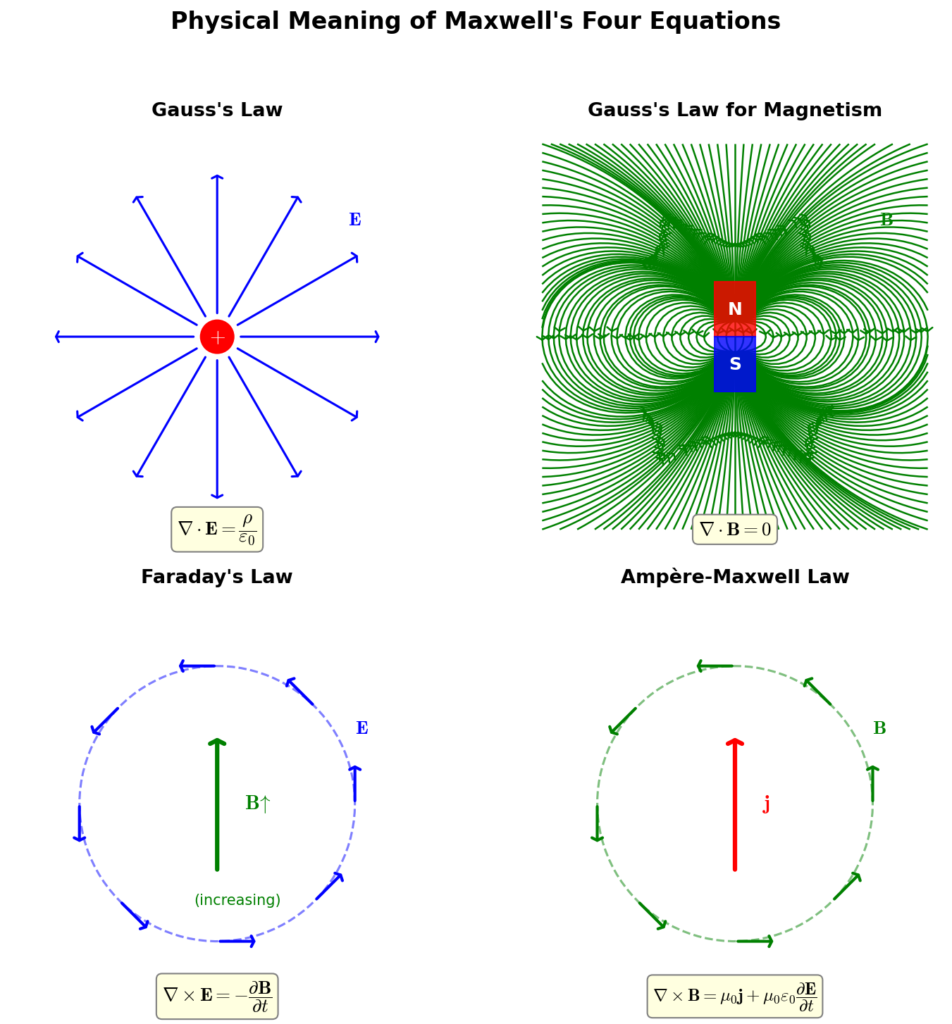
Fig. 2.5: Physical meaning of Maxwell's equations. Schematic diagrams of the physical situations described by each of Maxwell's equations.
The Necessity of the Displacement Current — Derivation from Charge Conservation
🟡 Lina: Let's write the law of charge conservation — "charge is neither created nor destroyed" — in equation form. Consider a small region. If current flows out of that region, the charge inside decreases, right?
🔵 Kai: Yes. It's like if water flows out of a bucket, the water inside decreases.
🟡 Lina: Exactly. \(\nabla \cdot \mathbf{j}\) is the divergence of current density — how much current is "flowing out" from a point. Current flowing out (\(\nabla \cdot \mathbf{j} > 0\)) means charge is leaving that location. So the charge density \(\rho\) decreases with time (\(\frac{\partial \rho}{\partial t} < 0\)).
🔵 Kai: The outflow is positive, but the rate of change of charge is negative... the signs are opposite.
🟡 Lina: Right. Using Kai's bucket analogy, when the water outflow (\(\nabla \cdot \mathbf{j}\)) is positive, the rate of change of water in the bucket (\(\frac{\partial \rho}{\partial t}\)) is negative — the signs are opposite. So \(\nabla \cdot \mathbf{j} = -\frac{\partial \rho}{\partial t}\). Rearranging gives the continuity equation:
⚪ Mei: In other words, "the charge in a region decreases by exactly the amount that flows out of it."
🟡 Lina: Right. Now, let's see what happens if the 4th equation were just the original Ampère's law — that is, only \(\nabla \times \mathbf{B} = \mu_0 \mathbf{j}\). Take the divergence \(\nabla \cdot\) of both sides:
🟡 Lina: The left side, by a vector calculus identity (see Appendix A), is always zero:
Therefore:
🔵 Kai: Wait — this says "the divergence of current is zero" — meaning "charge never accumulates or depletes"?
🟡 Lina: Exactly. But the continuity equation says \(\nabla \cdot \mathbf{j} = -\frac{\partial \rho}{\partial t}\). In situations where charge changes with time (for example, while charging a capacitor), \(\frac{\partial \rho}{\partial t} \neq 0\), so \(\nabla \cdot \mathbf{j} \neq 0\). There's a contradiction.
⚪ Mei: So the original Ampère's law alone is inconsistent with charge conservation.
🟡 Lina: So Maxwell added a term to the 4th equation to restore consistency. Taking the time derivative of both sides of the 1st equation \(\nabla \cdot \mathbf{E} = \rho/\varepsilon_0\):
Substituting the continuity equation \(\frac{\partial \rho}{\partial t} = -\nabla \cdot \mathbf{j}\):
Rearranging:
🔵 Kai: Ohh, \(\mathbf{j}\) alone doesn't have zero divergence, but when you add the time derivative of the electric field, it becomes zero!
🟡 Lina: Right. So \(\mathbf{j}\) alone doesn't have zero divergence, but \(\mathbf{j} + \varepsilon_0 \frac{\partial \mathbf{E}}{\partial t}\) does. So if we modify Ampère's law to:
then there's no longer a contradiction with \(\nabla \cdot (\nabla \times \mathbf{B}) = 0\).
⚪ Mei: The form of the term that needs to be added is uniquely determined just from mathematical consistency.
🟡 Lina: Right. This additional term \(\varepsilon_0 \frac{\partial \mathbf{E}}{\partial t}\) is called the displacement current. Maxwell didn't "discover it experimentally" — he derived it logically from the principle of charge conservation. I've made a figure showing why the displacement current is needed in a capacitor charging circuit (Fig. 2.6 "Conceptual diagram of displacement current").
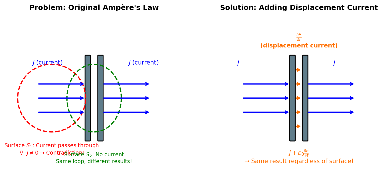
Fig. 2.6: Conceptual diagram of displacement current. While a capacitor is charging, no current flows between the plates but the electric field changes in time. With the original Ampère's law, the result depends on which surface you choose (left). Adding the displacement current \(\varepsilon_0 \partial_t E\) resolves the contradiction (right).
🟡 Lina: And this small correction will produce an extraordinary prediction.
✅ Comprehension Check: What does the second Maxwell equation \(\nabla \cdot \mathbf{B} = 0\) physically mean?
Answer
Magnetic field lines have no sources, and magnetic monopoles (isolated N pole or S pole) do not exist.
✅ Comprehension Check: On what basis was the term \(\mu_0 \varepsilon_0 \frac{\partial \mathbf{E}}{\partial t}\) that Maxwell added to the 4th equation (Ampère-Maxwell law) introduced?
Answer
It was introduced from the requirement of mathematical consistency with charge conservation (the continuity equation). The original Ampère's law alone contradicts charge conservation.
2.5 The Nature of Light — A Prediction from Maxwell's Equations
🟡 Lina: When you combine the 3rd and 4th Maxwell equations, here's what you find. A changing electric field generates a magnetic field, and that changing magnetic field generates an electric field again... this chain reaction continues, and an electromagnetic wave propagates through space.
%%{init: {"theme": "default", "themeCSS": ".edgePath .path, .flowchart-link { stroke-width: 2px !important; }"}}%%
flowchart LR
    E1["Change in E field"] -->|"4th eq: generates curl in B"| B1["Change in B field"]
    B1 -->|"3rd eq: generates curl in E"| E2["Change in E field"]
    E2 -->|"4th eq"| B2["Change in B field"]
    B2 -->|"3rd eq"| E3["…"]
Fig. 2.7: Electromagnetic wave propagation through mutual induction of E and B fields
🔵 Kai: A wave? Like a wave on water?
🟡 Lina: Similar, but water waves are vibrations of a medium — water. Electromagnetic waves propagate without a medium, with the electric and magnetic fields generating each other. Let's derive this explicitly.
Derivation of the Wave Equation
🟡 Lina: Writing out Maxwell's equations in vacuum (no charges or currents: \(\rho = 0\), \(\mathbf{j} = \mathbf{0}\)):
🟡 Lina: We want to create an equation for only the electric field \(\mathbf{E}\). The 3rd equation (III) contains \(\mathbf{B}\), but the 4th equation (IV) expresses \(\nabla \times \mathbf{B}\) in terms of the time derivative of \(\mathbf{E}\). So if we apply \(\nabla \times\) once more to both sides of the 3rd equation, the left side gives \(\nabla \times (\nabla \times \mathbf{E})\) and the right side produces \(\nabla \times \mathbf{B}\) — then we can substitute the 4th equation to eliminate \(\mathbf{B}\). Let's try:
🔵 Kai: You apply \(\nabla \times\) again to eliminate \(\mathbf{B}\). It's like building scaffolding for the substitution.
🟡 Lina: Right. On the right side, we swap the order of \(\nabla \times\) and \(\partial/\partial t\). Since \(\nabla \times\) is a differentiation with respect to spatial coordinates \((x,y,z)\) and \(\partial/\partial t\) is differentiation with respect to time — they're derivatives with respect to different variables, so swapping them doesn't change the result (\(\frac{\partial}{\partial t}\frac{\partial f}{\partial x} = \frac{\partial}{\partial x}\frac{\partial f}{\partial t}\)):
🟡 Lina: Substitute the 4th equation (IV) for \(\nabla \times \mathbf{B}\) on the right:
Simplifying:
🔵 Kai: The left side is \(\nabla \times (\nabla \times \mathbf{E})\) — the curl of the curl, right? How do you compute that?
🟡 Lina: Good question. We use a vector calculus identity (proven in Appendix A):
🔵 Kai: Hmm, the left side is "curl of the curl." What do the two terms on the right mean?
🟡 Lina: The first term on the right \(\nabla(\nabla \cdot \mathbf{E})\) represents "how the strength of the electric field's divergence varies from place to place," and the second term \(\nabla^2 \mathbf{E}\) is the Laplacian representing "how each component of the electric field curves spatially." But what matters for this derivation is not deeply understanding the physical meaning of this identity — it's the fact that in vacuum, the first term vanishes entirely. This is because, from equation (I), \(\nabla \cdot \mathbf{E} = 0\) in vacuum (no charges means no sources), so \(\nabla(\nabla \cdot \mathbf{E}) = \nabla(0) = \mathbf{0}\) and the first term vanishes. The identity itself can be verified by writing out the components (see Appendix A), but for now we'll just use the result "this decomposition exists":
⚪ Mei: The vacuum condition simplifies things beautifully.
🟡 Lina: Substituting this:
Multiplying both sides by \(-1\):
🟡 Lina: Here \(\nabla^2 \mathbf{E}\) is the "Laplacian of a vector field" explained in 2.3 "Scalar Fields and Vector Fields" — the scalar Laplacian \(\nabla^2\) applied to each component \(E_x, E_y, E_z\) separately, i.e., \((\nabla^2 E_x,\; \nabla^2 E_y,\; \nabla^2 E_z)\).
⚪ Mei: \(\mathbf{B}\) has completely disappeared, and we have an equation in \(\mathbf{E}\) alone.
🔵 Kai: The left side is a second spatial derivative and the right side is a second time derivative... But what does this have to do with "waves"?
🟡 Lina: Good question. The \(\nabla^2\) on the left is called the Laplacian operator — the sum of second spatial derivatives. Specifically:
Intuitively, it represents "how much the value at a point deviates from the average of its surroundings." For the electric field, it means "how the field curves spatially" (details in Appendix A). The \(\partial^2/\partial t^2\) on the right is the second time derivative — representing "how the electric field is accelerating in time."
🔵 Kai: This is the wave equation for the electric field, right? What about the magnetic field?
🟡 Lina: Good question. If you apply the same procedure to the magnetic field \(\mathbf{B}\), you get a wave equation of the same form. Applying \(\nabla \times\) to the 4th equation (IV) and doing the same calculation:
Both the electric and magnetic fields satisfy wave equations of the same form.
🔵 Kai: They give the same form of equation. So do the electric wave and magnetic wave propagate separately? Or together?
🟡 Lina: Together. Because the 3rd and 4th equations link them to each other, a wave of only electric field or only magnetic field cannot exist. They always propagate as a pair — that's why we call it an "electromagnetic wave."
⚪ Mei: I see. Since the 3rd equation says "changing B → curl in E" and the 4th says "changing E → curl in B," neither can exist alone.
🔵 Kai: But with water waves, you can see the water moving up and down. Electromagnetic waves have no "vibrating substance" but still propagate? Isn't that really strange?
🟡 Lina: That's precisely the point that 19th century physicists struggled with too. Many thought "there must be a medium (aether) that carries light." But the aether was never found — we'll cover this story in detail in Ch. 5.
🔵 Kai: So people back then had the same question. Then the modern view is that "the field itself oscillates"?
🟡 Lina: Yes. The electric and magnetic fields exist as entities in space, and they themselves oscillate and propagate — this is where Faraday's concept of the "field" comes into play.
The Wave Equation and Wave Speed
🟡 Lina: Let's compare the equation we just derived with a more general wave equation. In physics, when a "wave" propagates, its equation takes this form:
Here \(v\) is the propagation speed of the wave.
🔵 Kai: Why is this form a "wave"? I can't tell just from the appearance...
🟡 Lina: Good question. Let me show you concretely in the 1-dimensional case first:
For any shape of function \(g\), \(f(x,t) = g(x - vt)\) is a solution to this equation. Let's verify. Setting \(u = x - vt\), when differentiating with respect to \(x\): \(\frac{\partial u}{\partial x} = 1\) so \(\frac{\partial f}{\partial x} = g'(u)\), differentiating again gives \(\frac{\partial^2 f}{\partial x^2} = g''(u)\). Meanwhile, differentiating with respect to \(t\): \(\frac{\partial u}{\partial t} = -v\) so \(\frac{\partial f}{\partial t} = -v\,g'(u)\), differentiating again gives \(\frac{\partial^2 f}{\partial t^2} = v^2 g''(u)\). Therefore \(g''(u) = \frac{1}{v^2} \cdot v^2 g''(u)\), which indeed holds. This represents "the shape \(g\) moving to the right at speed \(v\) without changing" — that's why it's a "wave equation."
🔵 Kai: I see, it's the image of the waveform sliding sideways unchanged. But what specific shape of wave propagates?
🟡 Lina: A typical one is a periodic wave: \(f(x,t) = f_0 \sin(kx - \omega t)\). \(f_0\) is the amplitude — a constant representing the height of the wave crest. Two new symbols appear, so let me explain each one.
🟡 Lina: First, \(k\) (the wave number). Using the wavelength \(\lambda\) (the distance from one crest to the next), \(k = 2\pi/\lambda\). Why does \(2\pi\) appear? Because the \(\sin\) function completes one full oscillation when its argument changes by \(2\pi\). We define \(k\) so that when the distance increases by \(\lambda\), the change in \(kx\) is \(k\lambda = 2\pi\). The larger \(k\) is, the shorter the wavelength — meaning a finer wave.
🟡 Lina: Next, \(\omega\) (the angular frequency). If the frequency (number of oscillations per second) is \(\nu\), then \(\omega = 2\pi \nu\). For the same reason, it's defined so that after one period (\(1/\nu\) seconds), the change in \(\omega t\) is \(2\pi\). The larger \(\omega\) is, the faster the oscillation.
🔵 Kai: So \(k\) and \(\omega\) are quantities that absorb the \(2\pi\) so they can be directly plugged into the argument of \(\sin\)?
🟡 Lina: Exactly. Why do we try \(\sin\)? Because we already found that \(g(x - vt)\) is the general solution, and we're choosing the most basic periodic wave among those — one that repeats with a constant wavelength. \(\sin\) is the simplest function that "repeats smoothly with a constant wavelength," right? And in fact, it's mathematically proven that any complex waveform can be written as a superposition of \(\sin\) waves (called Fourier decomposition — see Quantum Mechanics Quantum Mechanics Appendix C for details). So studying the properties of \(\sin\) waves is sufficient.
⚪ Mei: The larger \(k\) is, the shorter the wavelength and the finer the wave; the larger \(\omega\) is, the faster the oscillation.
🟡 Lina: Right. Let's actually substitute \(f = f_0\sin(kx - \omega t)\) into the wave equation to verify. Differentiating once with respect to \(x\): \(\frac{\partial f}{\partial x} = k f_0\cos(kx - \omega t)\); differentiating again: \(\frac{\partial^2 f}{\partial x^2} = -k^2 f_0\sin(kx - \omega t) = -k^2 f\). Similarly, differentiating twice with respect to \(t\): \(\frac{\partial^2 f}{\partial t^2} = -\omega^2 f\).
🔵 Kai: The left side is \(-k^2 f\) and the right side is \(\frac{1}{v^2}(-\omega^2 f)\), so... for them to be equal, \(k^2 = \omega^2/v^2\), meaning \(v = \omega/k\)! But does this \(v\) change depending on the values of \(k\) or \(\omega\)? Do short-wavelength waves and long-wavelength waves all travel at the same speed?
🟡 Lina: Good question. For this wave equation, yes — \(v\) is determined as a constant within the equation, so it doesn't depend on \(k\) or \(\omega\). That means waves of any wavelength travel at the same speed. This property is called "no dispersion" (conversely, when speed depends on wavelength, we say there "is dispersion" — white light splitting into a rainbow through a prism happens because different wavelengths travel at different speeds in glass). Electromagnetic waves in vacuum have no dispersion; light of any wavelength travels at the same speed \(c\). Intuitively, "the greater the spatial curvature (left side), the more vigorous the temporal change (right side)" — this relationship generates waves. See Appendix A for details.
🟡 Lina: Comparing with the wave equation from Maxwell's equations:
Therefore, the speed of electromagnetic waves \(c\) is:
🔵 Kai: The wave speed is determined by just \(\mu_0\) and \(\varepsilon_0\).
🟡 Lina: I've shown how electromagnetic waves propagate in Fig. 2.8 "Orthogonal oscillation of E and B in an electromagnetic wave". The electric and magnetic fields oscillate perpendicular to each other and perpendicular to the direction of propagation.
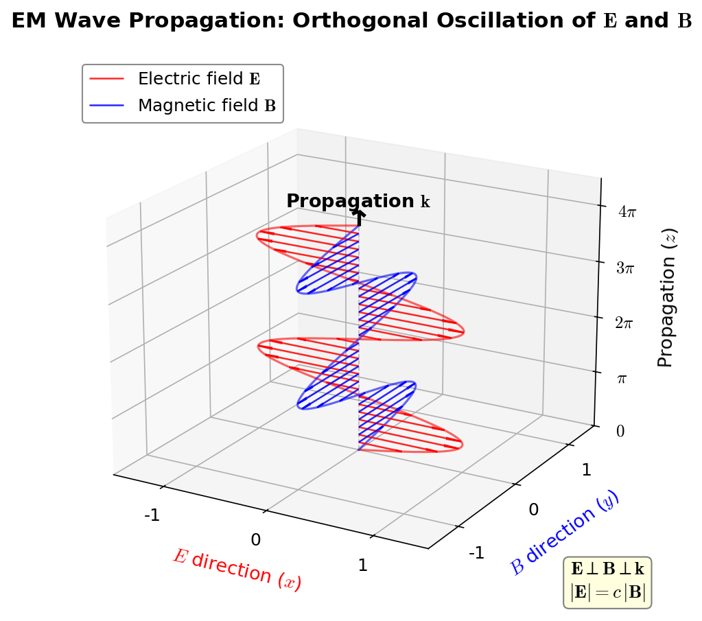
Fig. 2.8: Orthogonal oscillation of E and B in an electromagnetic wave. In an electromagnetic wave, the electric field E and magnetic field B oscillate perpendicular to each other and perpendicular to the direction of propagation.
Numerical Calculation of the Speed of Light
🟡 Lina: \(\mu_0\) and \(\varepsilon_0\) are constants that can be measured independently from electrical and magnetic experiments. Let's substitute their values:
Computing the product:
🔵 Kai: Why does the unit come out as \(\text{s}^2/\text{m}^2\)?
🟡 Lina: Let's check the units. The unit of \(\mu_0\) is \(\text{T·m/A}\). Tesla (T) is the unit of magnetic flux density, and decomposing into base units gives \(\text{T} = \text{kg/(A·s}^2\text{)}\) (this can be derived from the force equation \(\mathbf{F} = q\mathbf{v} \times \mathbf{B}\)). Substituting: \(\text{T·m/A} = \frac{\text{kg}}{\text{A·s}^2} \cdot \frac{\text{m}}{\text{A}} = \text{kg·m/(A}^2\text{·s}^2\text{)}\). The unit of \(\varepsilon_0\) is \(\text{C}^2/(\text{N·m}^2)\). Here \(\text{C} = \text{A·s}\) (coulomb = ampere × second), \(\text{N} = \text{kg·m/s}^2\), so \(\text{C}^2/(\text{N·m}^2) = (\text{A·s})^2/(\text{kg·m/s}^2 \cdot \text{m}^2) = \text{A}^2\text{·s}^4/(\text{kg·m}^3)\). Multiplying them: the unit of \(\mu_0\varepsilon_0\) is \(\frac{\text{kg·m}}{\text{A}^2\text{·s}^2} \times \frac{\text{A}^2\text{·s}^4}{\text{kg·m}^3} = \frac{\text{s}^2}{\text{m}^2}\). So the unit of \(1/\sqrt{\mu_0\varepsilon_0}\) is \(\text{m/s}\) — a unit of speed. The full steps of the unit conversion are in Appendix A, so check there if you'd like.
🔵 Kai: The key point is decomposing \(\text{N}\) into kilograms and meters.
⚪ Mei: We've confirmed the units come out as speed. Now for the numerical value.
Taking the reciprocal of the square root:
🔵 Kai: ...Isn't that the speed of light?! But why does combining constants from electricity and magnetism give the speed of light? Was light related to electricity and magnetism?
🟡 Lina: That's what's so shocking. Maxwell himself wrote: "The velocity is so nearly that of light that it seems we have strong reason to conclude that light itself is an electromagnetic disturbance." In other words, light is a wave of electric and magnetic fields — an electromagnetic wave.
⚪ Mei: A model that unified electricity and magnetism predicted that the nature of light is an electromagnetic wave.
🔵 Kai: Just like with Neptune... An unexpected discovery emerges from something unrelated to the original goal.
🟡 Lina: Yes. That's the power of "predictions from a model." Maxwell wasn't studying light. He was pursuing the unification of electricity and magnetism, and the nature of light was revealed as a byproduct. The same structure as when Neptune was predicted from Newton's model in Ch. 1.
📝 Exercises:
- Derivation of the wave equation from Maxwell's equations → Problem M-1. Derivation of Electromagnetic Wave Speed
- Numerical calculation of the speed of light → Problem B-1. Numerical Calculation of the Speed of Light
✅ Comprehension Check: What is the formula for the speed of electromagnetic waves \(c\) derived from Maxwell's equations, expressed in terms of \(\mu_0\) and \(\varepsilon_0\)?
Answer
\(c = \frac{1}{\sqrt{\mu_0 \varepsilon_0}}\)
✅ Comprehension Check: What did Maxwell's model predict about "the nature of light"?
Answer
That the nature of light is an electromagnetic wave. This was derived from the fact that the speed of electromagnetic waves matches the speed of light.
2.6 Electromagnetic Potentials and Gauge Transformations
🟡 Lina: Now let's rewrite the electric and magnetic fields in terms of potentials. This is the same idea as rewriting Newton's gravity in terms of the potential \(\Phi\) in Ch. 1. We can introduce potentials \((\Phi, \mathbf{A})\) for the electromagnetic field too.
Introduction of Potentials
🔵 Kai: The electric and magnetic fields have potentials too?
🟡 Lina: Yes. The starting point is Maxwell's 2nd equation \(\nabla \cdot \mathbf{B} = 0\). This says "the magnetic field has no sources." In vector calculus, there's the following identity:
🟡 Lina: That is, if \(\nabla \cdot \mathbf{B} = 0\) holds, then \(\mathbf{B}\) can be written as the curl of something:
This \(\mathbf{A}\) is called the vector potential.
🔵 Kai: "Having no sources" means "can be written as someone's curl" — it follows logically.
🟡 Lina: Right. Next, substitute this into the 3rd equation \(\nabla \times \mathbf{E} = -\frac{\partial \mathbf{B}}{\partial t}\):
Rearranging:
🟡 Lina: A vector field with "zero curl" can be written as the gradient of some scalar field (proof in Appendix A):
(The minus sign is convention.) Intuitively, "a flow with no swirl" necessarily has a structure of "flowing downhill" — it points in the direction of descending potential. Therefore:
Rearranging:
⚪ Mei: \(\Phi\) is the scalar potential (the same type as the gravitational potential from Ch. 1), and \(\mathbf{A}\) is the vector potential.
🟡 Lina: Right. In summary:
The advantage of this notation is that Maxwell's 2nd equation \(\nabla \cdot \mathbf{B} = 0\) and 3rd equation \(\nabla \times \mathbf{E} = -\partial_t \mathbf{B}\) are automatically satisfied. Two of the four equations come for free.
🔵 Kai: Two out of four automatically! Getting half for free is a big deal.
📝 Exercises:
- Verifying that \(\nabla \cdot \mathbf{B} = 0\) automatically holds from the vector potential → Problem B-2. From Potentials to Maxwell's Equations
Gauge Transformations — "Rewriting" That Doesn't Change the Physics
🔵 Kai: Is the potential uniquely determined? 🟡 Lina: Sharp question. In fact, it's not. Consider the following transformation:
Here \(\Lambda(\mathbf{r}, t)\) is an arbitrary scalar function. This transformation is called a gauge transformation.
⚪ Mei: Is it really okay to transform with an arbitrary function?
🟡 Lina: It is. Because what's physically observable are \(\mathbf{E}\) and \(\mathbf{B}\), not \(\Phi\) or \(\mathbf{A}\) themselves. Let's verify this explicitly.
🟡 Lina: First, the magnetic field. Compute the transformed \(\mathbf{B}'\):
🟡 Lina: Using the vector calculus identity \(\nabla \times (\nabla \Lambda) = \mathbf{0}\) (the curl of the gradient of any scalar field is zero):
The magnetic field is unchanged. ✓
🟡 Lina: Next, the electric field:
Expanding:
🔵 Kai: The 2nd and 4th terms have the same sign and... cancel?
🟡 Lina: Yes. Since \(\nabla\frac{\partial \Lambda}{\partial t} = \frac{\partial}{\partial t}(\nabla \Lambda)\) (swapping spatial and temporal derivatives), the 2nd and 4th terms cancel:
The electric field is also unchanged. ✓
🔵 Kai: Wow! No matter what \(\Lambda\) is, \(\mathbf{E}\) and \(\mathbf{B}\) are invariant.
%%{init: {"theme": "default", "themeCSS": ".edgePath .path, .flowchart-link { stroke-width: 2px !important; }"}}%%
flowchart TD
    A["Potential (Φ, A)"] -->|"E = -∇Φ - ∂A/∂t"| C["Electric field E"]
    A -->|"B = ∇×A"| D["Magnetic field B"]
    B["Potential (Φ', A')"] -->|"E = -∇Φ' - ∂A'/∂t"| C
    B -->|"B = ∇×A'"| D
    A <-->|"Gauge transformation\nΦ→Φ−∂ₜΛ\nA→A+∇Λ"| B
    style C fill:#f9f,stroke:#333
    style D fill:#f9f,stroke:#333
Fig. 2.9: Gauge transformations and the non-uniqueness of potentials
🟡 Lina: Right. The potentials \((\Phi, \mathbf{A})\) have redundancy. Infinitely many potentials describe the same physics (same \(\mathbf{E}\), \(\mathbf{B}\)). This redundancy is called gauge freedom.
✅ Comprehension Check: What is "gauge freedom"?
Answer
The redundancy that infinitely many potentials \((\Phi, \mathbf{A})\) describe the same physical situation (same \(\mathbf{E}\) and \(\mathbf{B}\)). Different potentials can be obtained by gauge transformations with an arbitrary scalar function \(\Lambda\), but physically observable quantities remain unchanged.
🔵 Kai: But if it's redundant, why bother using potentials at all? Can't we just write everything in terms of \(\mathbf{E}\) and \(\mathbf{B}\) directly?
🟡 Lina: Good question. There are two reasons. First, using potentials makes half of Maxwell's equations automatically satisfied, which simplifies calculations. Second — and this is the deeper reason — in quantum mechanics, the potential \(\mathbf{A}\) directly affects physics in situations where \(\mathbf{E}\) and \(\mathbf{B}\) do not (the Aharonov-Bohm effect, see Quantum Mechanics Quantum Mechanics Ch. 26).
⚪ Mei: So a "seemingly redundant description" is actually necessary for describing deeper physics.
🟡 Lina: And this gauge freedom isn't just a mathematical convenience — it reflects a fundamental symmetry of nature. In Ch. 9, where we study gauge symmetry and the Standard Model, and all the way to string theory in Part IV, the concept of gauge transformations will appear again and again.
Philosophy of Science Note: Gauge transformations use a descriptive framework that contains "physically unobservable degrees of freedom." This raises the philosophical question of "the distinction between model description and physical reality." Are potentials "real," or are they merely convenient computational tools? The answer to this question changes after the advent of quantum mechanics. The materials for making your own judgment will accumulate as you continue reading this book.
✅ Comprehension Check: What is the formula for obtaining the magnetic field \(\mathbf{B}\) from the electromagnetic potentials \((\Phi, \mathbf{A})\)?
Answer
\(\mathbf{B} = \nabla \times \mathbf{A}\)
✅ Comprehension Check: Under the gauge transformation \(\Phi \to \Phi - \partial_t \Lambda\), \(\mathbf{A} \to \mathbf{A} + \nabla\Lambda\), what happens to \(\mathbf{E}\) and \(\mathbf{B}\)?
Answer
Both remain invariant (unchanged). Physically observable quantities do not change under gauge transformations.
2.7 Lagrangian Formulation (Advanced)
🟡 Lina: From here the content becomes more advanced — you can skip this entire section on first reading and proceed to Ch. 3. No subsequent chapter assumes knowledge of this section, so don't worry. If you return after learning special relativity in Ch. 5, the 4-dimensional notation will make much more sense. However, reading it now reveals that "the 4 Maxwell equations that appear separate actually all emerge from a single action" — the deepest expression of "unification," which is the theme of this chapter. In Ch. 1, we introduced the "action principle." Newton's equation of motion can be derived from the stationarity condition of the action \(S\). The same thing can be done for Maxwell's equations.
🔵 Kai: Maxwell's equations also come from the action principle?
🟡 Lina: Yes. To do this, we first need to introduce a tool called the electromagnetic field tensor \(F_{\mu\nu}\). This uses the language of 4-vectors that you'll learn in General Relativity General Relativity Ch. 3.
The 4-Potential and the Electromagnetic Field Tensor
🟡 Lina: The goal of this subsection is to see that "the electric and magnetic fields are actually different components of a single object (a tensor)." To do this, we introduce 4-dimensional notation that unifies time and space.
🟡 Lina: In special relativity, time and space are unified and written with 4-dimensional coordinates \(x^\mu = (ct, x, y, z)\). Similarly, we combine the scalar potential \(\Phi\) and vector potential \(\mathbf{A}\) into a single 4-potential:
🟡 Lina: In contravariant components (upper index):
Here \(A_x, A_y, A_z\) are exactly the components of the 3-dimensional vector potential \(\mathbf{A} = (A_x, A_y, A_z)\) used in the previous section.
🔵 Kai: Why \(\Phi/c\) instead of just \(\Phi\)?
🟡 Lina: Because all components of a 4-vector need to have the same dimensions (units). The unit of \(\mathbf{A}\) is \(\text{V·s/m}\) (which follows from \(\mathbf{B} = \nabla \times \mathbf{A}\)). The unit of \(\Phi\) is \(\text{V}\), so \(\Phi/c\) gives \(\text{V/(m/s)} = \text{V·s/m}\), matching \(\mathbf{A}\).
🔵 Kai: What do "contravariant" and "covariant" mean? Why do we need two kinds of notation?
🟡 Lina: Good question. You'll learn the details in General Relativity General Relativity Ch. 3, but for now just remember the computational rule that "whether the index is up or down changes the sign of spatial components." The reason will click when you learn special relativity in Ch. 5.
🟡 Lina: In one sentence, why two kinds are needed: when treating time and space within a single framework, a "weight" is needed to distinguish them. In everyday terms, "traveling 3 km north" and "waiting 3 hours" are physically completely different even though both involve "3," right? When writing time and space side by side in 4 dimensions, we express that difference with signs — that's the metric tensor \(\eta_{\mu\nu}\). It's a 4×4 matrix with values only on the diagonal, specifically \(\eta_{\mu\nu} = \begin{pmatrix} +1 & 0 & 0 & 0 \\ 0 & -1 & 0 & 0 \\ 0 & 0 & -1 & 0 \\ 0 & 0 & 0 & -1 \end{pmatrix}\). So the rule is: multiply the time component (\(\mu = \nu = 0\)) by \(+1\), and spatial components (\(\mu = \nu = 1, 2, 3\)) by \(-1\).
⚪ Mei: The "difference in weight" between time and space is expressed through signs.
🟡 Lina: In contravariant components (upper index), the 3-dimensional components enter as-is. Covariant components (lower index) are obtained via \(A_\mu = \eta_{\mu\nu}A^\nu\). Since the spatial components get multiplied by \(-1\), their signs flip:
🟡 Lina: And we define the electromagnetic field tensor as:
Here \(\partial_\mu = \frac{\partial}{\partial x^\mu}\). Note that since all indices in the definition are lower (covariant), we use the covariant components \(A_\mu = (\Phi/c, -A_x, -A_y, -A_z)\) for the calculation.
🔵 Kai: I understand the definition, but what does it concretely compute to?
🟡 Lina: When you write out the components of \(F_{\mu\nu}\), the electric and magnetic fields emerge. For example:
🟡 Lina: Since all indices in the definition of \(F_{\mu\nu}\) are lower (covariant), we use the covariant components \(A_\mu = (\Phi/c, -A_x, -A_y, -A_z)\). Since \(x^0 = ct\), we have \(\partial_0 = \frac{\partial}{\partial x^0} = \frac{\partial}{\partial(ct)} = \frac{1}{c}\frac{\partial}{\partial t}\). Similarly \(\partial_1 = \frac{\partial}{\partial x^1} = \frac{\partial}{\partial x}\). Substituting \(A_0 = \Phi/c\) and \(A_1 = -A_x\):
Recalling from the previous section that \(E_x = -\frac{\partial \Phi}{\partial x} - \frac{\partial A_x}{\partial t}\), multiplying both sides by \(-1\) gives \(\frac{\partial \Phi}{\partial x} + \frac{\partial A_x}{\partial t} = -E_x\), so:
🔵 Kai: The electric field appears as a component of the tensor!
🟡 Lina: Computing similarly, \(F_{\mu\nu}\) becomes an antisymmetric tensor containing all components of both the electric and magnetic fields. That is, the 6 components of \(\mathbf{E}\) and \(\mathbf{B}\) are packaged into a single tensor \(F_{\mu\nu}\).
🔵 Kai: The electric and magnetic fields are combined into a single object.
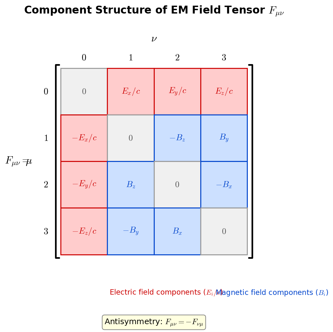
Fig. 2.10: Component structure of the electromagnetic field tensor. Shows how the electric and magnetic fields are stored in the components of the antisymmetric tensor F_μν.
🟡 Lina: Yes. This is the mathematical expression of "the unification of electricity and magnetism." When you change coordinates by a Lorentz transformation (see General Relativity General Relativity Ch. 3), the components of \(F_{\mu\nu}\) mix — meaning what one observer calls "electric field" appears as part of the "magnetic field" to another observer. The electric and magnetic fields are different aspects of the same thing.
Gauge Transformation in 4 Dimensions
🟡 Lina: Let's write the gauge transformation we learned earlier in 4-dimensional language. However, one note of caution. The covariant components of the 4-potential have \(A_\mu = (\Phi/c, -A_x, -A_y, -A_z)\) with a minus sign on spatial components, so matching the signs with the 3-dimensional version requires some care.
🔵 Kai: The signs seem like they could get confusing...
🟡 Lina: They can. In fact, different textbooks use different sign conventions. So for now, let's grasp only the essence. The essence is "the electromagnetic field tensor \(F_{\mu\nu}\) is invariant under gauge transformations" — that's all. Let's confirm that first, then look at the correspondence with the 3-dimensional version as a supplement. We write the 4-dimensional gauge transformation as:
(\(\chi\) is an arbitrary scalar function). Why do we use a different symbol from the 3-dimensional \(\Lambda\)? Because in 4 dimensions, the form "add \(\partial_\mu\chi\) to the covariant component \(A_\mu\)" is the simplest — it has the relation \(\chi = -\Lambda\) with the 3-dimensional \(\Lambda\), which we'll verify later. Applying this transformation to \(F_{\mu\nu} = \partial_\mu A_\nu - \partial_\nu A_\mu\):
🟡 Lina: Since partial derivatives commute (\(\partial_\mu \partial_\nu \chi = \partial_\nu \partial_\mu \chi\)), the extra terms cancel:
The electromagnetic field tensor is gauge invariant. ✓
🔵 Kai: I see, it has the same structure as the 3-dimensional version — the extra terms cancel and the physical quantity doesn't change. But how does it correspond to the 3-dimensional gauge transformation \(\Phi \to \Phi - \partial_t\Lambda\), \(\mathbf{A} \to \mathbf{A} + \nabla\Lambda\)?
🟡 Lina: Setting \(\chi = -\Lambda\) gives agreement with the 3-dimensional version. The sign is opposite because the spatial part of the covariant components \(A_\mu\) has a minus sign: \(A_i = -A_i^{\text{(3D)}}\), so \(\partial_i\chi = -\partial_i\Lambda\) in \(A_i + \partial_i\chi\) corresponds to \(\mathbf{A} + \nabla\Lambda\) in 3D. Checking the \(\mu = 0\) component: \(\Phi/c \to \Phi/c + \frac{1}{c}\partial_t(-\Lambda) = \Phi/c - \frac{1}{c}\partial_t\Lambda\), giving \(\Phi \to \Phi - \partial_t\Lambda\). For spatial components: \(A_i \to A_i + \partial_i\chi = -A_x + (-\partial_x\Lambda)\), so in terms of the 3-dimensional vector potential: \(A_x \to A_x + \partial_x\Lambda\) — indeed reproducing \(\mathbf{A} \to \mathbf{A} + \nabla\Lambda\). ✓
⚪ Mei: So the only difference between the 3-dimensional and 4-dimensional versions is the sign of the function used, and the physics is the same.
🟡 Lina: Exactly. Different textbooks use different conventions for \(\chi\) vs. \(\Lambda\), but what you should remember at this stage is: \(F_{\mu\nu}\) is invariant under gauge transformations — that's the essence. The details of sign conventions will be organized again in General Relativity General Relativity Ch. 3.
The Electromagnetic Lagrangian Density
🟡 Lina: To write the action for the electromagnetic field, we define the Lagrangian density. The simplest quantity that is both gauge invariant and Lorentz invariant is:
🔵 Kai: Why is there a \(-\frac{1}{4\mu_0}\)?
🟡 Lina: The coefficient \(-\frac{1}{4\mu_0}\) is a normalization chosen so that when you derive the Euler-Lagrange equations from this Lagrangian, you get exactly Maxwell's equations in SI units. In natural units (\(c = 1\) plus \(\mu_0 = 1\) — meaning electromagnetic units are also taken to "natural" sizes), it becomes simply \(-\frac{1}{4}\).
🟡 Lina: When you expand \(F_{\mu\nu}F^{\mu\nu}\) in components, it becomes a combination of squares of electric and magnetic field components. However, writing out \(c\) and \(\mu_0\) every time makes the expressions long and obscures the essence. So to make calculations concise, we'll use natural units (a unit system where \(c = 1\), \(\mu_0 = 1\)). In our earlier calculation, \(F_{01} = E_x/c\), but with \(c = 1\) this becomes \(F_{01} = E_x\) — the expressions become much cleaner, right?
🔵 Kai: Is it really okay to set constants to 1? Don't the values of physical quantities change?
🟡 Lina: Good question. This isn't "changing the values of constants" — it's "changing the choice of units." For example, measuring distance in km vs. m changes the numerical value but not the physics, right? Similarly, if you take the unit of length to be "the distance light travels in 1 second," then \(c = 1\). Setting \(\mu_0 = 1\) follows the same logic — by appropriately redefining the unit of current, \(\mu_0\) becomes 1. It just makes expressions cleaner, and if you want to convert back to SI units at the end, you can restore \(c\) and \(\mu_0\) through dimensional analysis (details in General Relativity General Relativity Ch. 3).
⚪ Mei: In programming terms, it's like storing constants in variable names and referencing them later. The values themselves haven't changed.
🟡 Lina: In this unit system, \(F_{01} = E_x\) (from our earlier \(E_x/c\) with \(c=1\)), and the Lagrangian density becomes \(\mathcal{L}_{\text{EM}} = -\frac{1}{4}F_{\mu\nu}F^{\mu\nu}\). Here \(F^{\mu\nu}\) is obtained by raising indices with the metric: \(F^{\mu\nu} = \eta^{\mu\alpha}\eta^{\nu\beta}F_{\alpha\beta}\).
🔵 Kai: What does "raising indices with the metric" mean?
🟡 Lina: When the same index \(\alpha\) appears once up and once down, you sum over that index from 0 to 3 — this is called Einstein's summation convention. For example, \(\eta^{\mu\alpha}F_{\alpha\beta}\) is shorthand for \(\sum_{\alpha=0}^{3}\eta^{\mu\alpha}F_{\alpha\beta}\).
🔵 Kai: So when \(\alpha\) appears both up and down, it means "sum over \(\alpha = 0, 1, 2, 3\)"?
🟡 Lina: Yes. Written explicitly: \(\eta^{\mu\alpha}F_{\alpha\beta} = \eta^{\mu 0}F_{0\beta} + \eta^{\mu 1}F_{1\beta} + \eta^{\mu 2}F_{2\beta} + \eta^{\mu 3}F_{3\beta}\) — summing all 4 terms. But since the metric \(\eta_{\mu\nu} = \mathrm{diag}(+1,-1,-1,-1)\) is a diagonal matrix, \(\eta^{\mu\alpha}\) is nonzero only when \(\alpha = \mu\), and zero otherwise. So even after summing, only the \(\alpha = \mu\) term survives. The result is the operation "time component stays the same, spatial components flip sign."
🔵 Kai: Since it's a diagonal matrix, you essentially just pick out that component.
🟡 Lina: Right. Let me do one concrete example. To find \(F^{01}\), compute \(F^{01} = \eta^{00}\eta^{11}F_{01}\) (since the matrix is diagonal, only the \(\alpha = 0\), \(\beta = 1\) term survives). \(\eta^{00} = +1\), \(\eta^{11} = -1\), so \(F^{01} = (+1)(-1)E_x = -E_x\). So "raising an index" flips the sign for spatial directions. Why this sign convention exists will become natural when you learn special relativity in General Relativity General Relativity Ch. 3 — for now, accept it as a "computational rule." This sign flip matters when expanding \(F_{\mu\nu}F^{\mu\nu}\). Using the metric \(\eta_{\mu\nu} = \mathrm{diag}(+1,-1,-1,-1)\) and summing over all components (everything below is in natural units \(c = 1\), \(\mu_0 = 1\)):
🔵 Kai: Why does \(\mathbf{E}^2\) get a minus sign? And where does the 2 come from?
🟡 Lina: Let me give you just the key points. When raising indices with the metric \(\eta^{\mu\nu}\), time-space components (e.g., \(F_{01} = E_x\)) get multiplied by \(\eta^{00}\eta^{11} = (+1)(-1) = -1\). So \(F_{01}F^{01} = E_x \cdot (-E_x) = -E_x^2\) — the electric field contribution is negative. On the other hand, space-space components (e.g., \(F_{12} = B_z\)) get \(\eta^{11}\eta^{22} = (-1)(-1) = +1\), so \(F_{12}F^{12} = B_z^2\) — the magnetic field contribution is positive.
🔵 Kai: The metric signs \((+1,-1,-1,-1)\) are what matter here.
🟡 Lina: Right. For the "2," let me show you concretely. \(F_{\mu\nu}F^{\mu\nu}\) sums over all \(\mu\) and \(\nu\) from 0 to 3 — so it includes both the \(\mu = 0, \nu = 1\) term and the \(\mu = 1, \nu = 0\) term. By antisymmetry \(F_{10} = -F_{01}\), we get \(F_{10}F^{10} = (-E_x)(+E_x) = -E_x^2\), which equals \(F_{01}F^{01} = -E_x^2\). So the same physical component is counted twice. Writing in terms of independent components gives a factor of 2. The full expansion details are in Appendix A — check there if interested.
Therefore:
🔵 Kai: Electric field squared minus magnetic field squared... Does it have a similar form to \(L = T - V\) from Ch. 1?
🟡 Lina: Good intuition. It has a similar structure to the particle mechanics Lagrangian \(L = T - V\) (kinetic energy minus potential energy), right? You can think of the electric field as the "kinetic" part and the magnetic field as the "potential" part. The precise correspondence is covered in Quantum Field Theory Quantum Field Theory Ch. 3.
⚪ Mei: So the same "something minus something" form we saw in Ch. 1 as \(T - V\) repeats in field theory too.
Re-deriving Maxwell's Equations from the Action Principle (Overview)
🟡 Lina: The action is:
Here \(d^4x = dt\,dx\,dy\,dz\) represents a 4-dimensional integral over all of time and space. Using coordinates \(x^\mu = (ct, x, y, z)\), this can be written as \(d^4x = \frac{1}{c}dx^0\,dx^1\,dx^2\,dx^3\) (in natural units \(c=1\), both forms are the same).
🟡 Lina: In Ch. 1, we learned the Euler-Lagrange equation for particles: \(\frac{d}{dt}\frac{\partial L}{\partial \dot{q}} - \frac{\partial L}{\partial q} = 0\). In field theory, the field \(A_\nu(x)\) becomes the dynamical variable instead of the particle position \(q(t)\). The corresponding Euler-Lagrange equation for fields is (derivation covered in detail in Quantum Field Theory Quantum Field Theory Ch. 3):
🔵 Kai: For particles, we had \(\frac{\partial L}{\partial \dot{q}}\) — "differentiate with respect to velocity." In the field case, what is \(\frac{\partial \mathcal{L}}{\partial(\partial_\mu A_\nu)}\) differentiating with respect to?
🟡 Lina: Good question. It's the same idea as treating \(\dot{q}\) as a variable independent of \(q\) when computing \(\frac{\partial L}{\partial \dot{q}}\) in particle mechanics. In the field case, you treat \(\partial_\mu A_\nu\) (each derivative component of the field) as independent variables and take partial derivatives of \(\mathcal{L}\) with respect to them. But since in the field case \(\partial_\mu A_\nu\) has multiple components for \(\mu = 0,1,2,3\) and \(\nu = 0,1,2,3\), you're specifying "which \(\mu\), \(\nu\) combination of derivative component to differentiate with respect to."
🔵 Kai: For particles, there was just one \(\dot{q}\), but for fields there are many derivative components.
🟡 Lina: Right. Let me show one concrete example. Within \(\mathcal{L} = -\frac{1}{4}F_{\alpha\beta}F^{\alpha\beta}\), we have \(F_{01} = \partial_0 A_1 - \partial_1 A_0\). When differentiating with respect to \(\partial_0 A_1\), only the \(\partial_0 A_1\) inside \(F_{01}\) responds and returns 1, while the \(\partial_1 A_0\) part gives zero. The result is a term proportional to \(F^{01}\) — you do this calculation for all combinations of \(\mu\) and \(\nu\). And the \(\partial_\mu\) in the first term uses the summation convention to sum over \(\mu = 0, 1, 2, 3\) — meaning it adds up derivatives in all spacetime directions.
⚪ Mei: So in particle mechanics, \(\frac{d}{dt}\) was only in the time direction, but in field theory it becomes a sum over all directions.
🟡 Lina: Right. Whereas particle mechanics had \(\frac{d}{dt}\) only in the time direction, field theory has \(\partial_\mu\) — a sum of derivatives in all spacetime directions — that's the key point of extending from particles to fields.
🔵 Kai: For particles we differentiated with respect to \(q\) and \(\dot{q}\). For fields we differentiate with respect to \(A_\nu\) and \(\partial_\mu A_\nu\)... So "the field value" and "the field's spatial/temporal rate of change" correspond to each other?
🟡 Lina: Yes, good understanding. Comparing with the particle mechanics equation, the correspondence is \(\frac{d}{dt} \to \partial_\mu\), \(\dot{q} \to \partial_\mu A_\nu\), \(q \to A_\nu\). Since \(\mathcal{L}_{\text{EM}} = -\frac{1}{4}F_{\mu\nu}F^{\mu\nu}\) (in vacuum) depends only on \(\partial_\mu A_\nu\) and not on \(A_\nu\) itself, the second term is zero. In the first term, we differentiate \(\mathcal{L}\) with respect to \(\partial_\mu A_\nu\), which means differentiating the \(\partial_\mu A_\nu\) inside \(F_{\mu\nu}F^{\mu\nu}\), yielding \(F^{\mu\nu}\). The calculation gives (details of derivation in Quantum Field Theory Quantum Field Theory Ch. 3):
🔵 Kai: Maxwell's equations in just one line...!
🟡 Lina: This is Maxwell's equations in vacuum (the vacuum versions of the 1st and 4th equations) written in 4-dimensional language. Since \(\nu\) takes values 0, 1, 2, 3, it actually contains 4 equations. Taking \(\nu = 0\) gives \(\partial_i F^{i0} = 0\), which corresponds to \(\nabla \cdot \mathbf{E} = 0\) (the 1st equation in vacuum). Taking \(\nu = 1, 2, 3\) corresponds to \(\nabla \times \mathbf{B} = \mu_0\varepsilon_0 \frac{\partial \mathbf{E}}{\partial t}\) (the 4th equation in vacuum). When charges and currents are present, you add a coupling term \(-A_\nu j^\nu\) to the Lagrangian. Then \(\mathcal{L}\) depends on \(A_\nu\) as well, and the second term of the Euler-Lagrange equation produces \(j^\nu\). Restoring SI units (restoring \(\mu_0\)):
Here \(j^\nu = (c\rho, \mathbf{j})\) is the 4-current density.
🔵 Kai: Amazing. All 4 Maxwell equations emerge naturally from the action principle.
🟡 Lina: Yes. In Ch. 1, the equation of motion for particles came from the action principle, right? Now field equations also come from the same principle — the action principle is a universal framework that works for both particles and fields.
⚪ Mei: The same structure repeats. For both particles and fields, write a Lagrangian and vary it to get equations of motion.
🟡 Lina: And the reason this Lagrangian formulation is important is that it becomes the starting point when quantizing the electromagnetic field in quantum field theory (Quantum Field Theory Quantum Field Theory Ch. 6). Furthermore, in string theory (Ch. 13 onward), the action principle plays a central role. The structure we've seen here will be used all the way through.
Philosophy of Science Note: The Lagrangian \(\mathcal{L} = -\frac{1}{4}F_{\mu\nu}F^{\mu\nu}\) is almost uniquely determined by just the requirements of "gauge invariance," "Lorentz invariance," and "yielding at most second-order differential equations." Symmetry requirements determine the form of the theory — this is the seed of the gauge principle, a theme that will be fully developed in Ch. 9.
✅ Comprehension Check: What is the definition of the electromagnetic field tensor \(F_{\mu\nu}\)?
Answer
\(F_{\mu\nu} = \partial_\mu A_\nu - \partial_\nu A_\mu\)
✅ Comprehension Check: What do you obtain by deriving the Euler-Lagrange equations from the electromagnetic Lagrangian density \(\mathcal{L}_{\text{EM}} = -\frac{1}{4}F_{\mu\nu}F^{\mu\nu}\)?
Answer
Maxwell's equations in vacuum: \(\partial_\mu F^{\mu\nu} = 0\).
2.8 Remaining Questions — Foreshadowing
🟡 Lina: Maxwell's model unified electricity, magnetism, and light. But it also gave birth to new mysteries.
🔵 Kai: What kind?
🟡 Lina: The problem that the speed of light \(c\) is "the same for everyone."
🔵 Kai: The speed of light is the same for everyone — what does that mean? If you throw a ball inside a moving train, its speed looks different from the ground versus from inside the train, right?
🟡 Lina: Right. Normally, the speed of a wave changes depending on the observer's state of motion. But the speed of light \(c = 1/\sqrt{\mu_0 \varepsilon_0}\) derived from Maxwell's equations contains no information about "as seen by whom." \(\mu_0\) and \(\varepsilon_0\) are constants representing properties of the vacuum and don't depend on the observer's velocity.
🔵 Kai: So if you run alongside light in the same direction and look at it, light should appear slower... but Maxwell's equations don't say that?
🟡 Lina: Right. Maxwell's equations simply say "the speed of light is \(c\)." They don't specify "as measured by whom it is \(c\)." This directly contradicts the common sense of Newtonian mechanics — that velocity depends on the observer. Einstein's special relativity (Ch. 5) is what resolved this contradiction.
🔵 Kai: So you think you've achieved unification, and then the next problem appears. It never ends...
🟡 Lina: It seems never-ending, but there's actually a pattern.
🔵 Kai: A pattern?
🟡 Lina: Newton unified gravity, and "why does it propagate instantaneously?" remained. Maxwell unified electromagnetism, and "why is the speed of light the same for everyone?" remained. Each time we unify, a new question emerges that wasn't visible in the previous model.
🔵 Kai: So when you solve the "remaining question," does yet another new question appear? If it goes on forever, does an ultimate unification really exist?
🟡 Lina: That's one of the fundamental questions of physics. Does an "ultimate theory" exist, or is it an infinite nested structure? At the end of this book (Part IV), we'll see how string theory attempts to answer that question.
⚪ Mei: But at the very least, each unification makes "what we don't know" clearer.
🔵 Kai: But at minimum, "what to ask next" becomes clear with each unification. With Newton, "why does it propagate instantaneously?" remained, and with Maxwell, "why is the speed of light constant?" remained — both are questions about "speed." Is that a coincidence?
🟡 Lina: Good catch. It's not a coincidence. There's a structure where each unification sharpens questions about how information propagates. And that structure itself becomes the driving force that pushes physics forward.
🟡 Lina: And let me plant one more seed. The gauge transformation freedom that appeared in this chapter — that's not just a mathematical convenience, but reflects a deep symmetry of nature.
⚪ Mei: The "redundant description" of potentials has such deep meaning.
🟡 Lina: In Ch. 9, we'll learn that the gauge transformation seen in this chapter is a manifestation of a mathematical structure called "\(U(1)\) gauge symmetry," and we'll see the path to the Standard Model by extending it further (the meaning of symbols like \(U(1)\) is defined in Ch. 9; for details see Quantum Field Theory Quantum Field Theory Ch. 17).
%%{init: {"theme": "default", "themeCSS": ".edgePath .path, .flowchart-link { stroke-width: 2px !important; }"}}%%
flowchart TD
    A["Laws of electricity\n(Coulomb)"] --> C["Maxwell's equations\nUnified into 4 equations"]
    B["Laws of magnetism\n(Ampère, Faraday)"] --> C
    D["Charge conservation"] -->|"Introduction of displacement current"| C
    C -->|"Derive wave equation"| E["Prediction of EM waves\nc = 1/√(μ₀ε₀)"]
    E --> F["Light is an electromagnetic wave"]
    C -->|"Potential formulation"| G["(Φ, A) and gauge transformations"]
    G --> H["Gauge symmetry\n→ Chapter 9: Standard Model"]
    F --> I["Mystery of light speed invariance\n→ Chapter 5: Special Relativity"]
    C --> J["Unification with gravity unachieved\n→ Part IV: String Theory"]
Fig. 2.11: Logical structure from Maxwell's equations to the prediction of light
✅ Comprehension Check: What is the new mystery generated by the speed of light \(c = 1/\sqrt{\mu_0 \varepsilon_0}\) derived from Maxwell's equations?
Answer
The problem that the speed of light \(c\) contains no information about "as seen by whom" and takes the same value regardless of the observer's state of motion.
Preview of the Next Chapter
Ch. 3「Making Steam Engines More Efficient — The Birth of Thermodynamics and Entropy」 — The story of Carnot pursuing the efficiency limits of steam engines, and Boltzmann uncovering the statistical meaning of entropy. An investigation that began from "necessity" arrives at fundamental properties of the universe.
References
The content of this chapter was structured based on the following references.
- David Tong, Lectures on Quantum Field Theory, Ch.2: "Free Fields" — Lagrangian formulation of Maxwell's equations, field strength tensor \(F_{\mu\nu}\)
- Lee Smolin, The Trouble with Physics, Ch.3: "The World As Geometry" — Historical motivation for unification and evaluation criteria
- Lee Smolin, The Trouble with Physics, Ch.4: "Unification Becomes a Science" — Foreshadowing of gauge symmetry, \(U(1)\) gauge theory
- J.D. Jackson, Classical Electrodynamics, Ch.6 — Maxwell's equations, derivation of the wave equation
- D.J. Griffiths, Introduction to Electrodynamics, Ch.7 — Electromagnetic waves, potentials and gauge transformations
Feedback on this page
Let us know if something was unclear, incorrect, or could be improved.