Appendix B Tensor Products, Components, and Contraction Notation Summary
Story so far:
In Appendix A, we organized vector analysis in 3-dimensional Euclidean space—vector products, differential operators (grad, div, curl, Laplacian), and integral theorems (Gauss's theorem, Stokes' theorem)—with proofs. We made these tools available as a "dictionary" to serve as the foundation for tensor calculations in the main text.
Goals of this chapter
- Understand the definition and computational rules (distributive law, non-commutativity) of the tensor product \(\otimes\), and grasp the structure of the contravariant tensor space \(T^r(V)\)
- Furthermore, acquire the coordinate-independent perspective of viewing tensors as "multilinear maps," and understand the relationship with covariant tensors (such as the metric tensor). Become proficient in using Einstein's summation convention freely
- These are essential tools for handling multi-index quantities such as the metric tensor and Riemann tensor that appear in the main text
B.1 Why Are Tensor Products Necessary?
🟡 Lina: So far, we've learned about vectors and 1-forms. Vectors are "quantities with one upper index," and 1-forms are "quantities with one lower index." But in the Einstein equation
quantities with two lower indices appear. The Riemann tensor \(R^\rho{}_{\sigma\mu\nu}\) has as many as four indices.
🔵 Kai: So having more indices means vectors alone aren't enough.
🟡 Lina: Right. Vectors are "rank-1" tensors—quantities with one index. To systematically handle quantities with two or more indices, we need an operation that builds a larger space from a vector space. That operation is the tensor product \(\otimes\). In other words, the tensor product is the mathematical tool for "increasing the number of indices." Today, we'll start by thoroughly learning the computational rules of tensor products.
⚪ Mei: I see, since vectors alone can only handle one index, we need an operation to create quantities with more indices.
B.2 Constructing the Tensor Product Space
🟡 Lina: Let's consider a 2-dimensional linear space \(V\) with basis \(e_1, e_2\). We want to construct the tensor product \(V \otimes V\) of \(V\) with itself. The method is straightforward. We combine \(e_1, e_2\) in pairs of two to create
these 4 symbols. The linear space formed by taking these 4 as a basis with real number coefficients is \(V \otimes V\).
🔵 Kai: Four basis elements, so it's a 4-dimensional linear space?
🟡 Lina: Exactly. If \(V\) is 2-dimensional, then \(V \otimes V\) is \(2 \times 2 = 4\) dimensional. If \(V\) is \(n\)-dimensional, then \(V \otimes V\) is \(n^2\)-dimensional.
✅ Comprehension Check: What is the dimension of the tensor product space \(V \otimes V\) for an \(n\)-dimensional vector space \(V\)? What form do its basis elements take?
Answer
The dimension of \(V \otimes V\) is \(n^2\). The basis consists of \(n^2\) elements of the form \(e_i \otimes e_j\) (\(i, j = 1, \ldots, n\)). These are formed by combining pairs of basis vectors of \(V\) connected by \(\otimes\).
⚪ Mei: What exactly is \(e_1 \otimes e_2\) as an object?
🟡 Lina: Honestly, you don't need to worry about what it really is. Understanding it as "something made by lining up \(e_1\) and \(e_2\) in order and gluing them together" is sufficient. What matters isn't the identity but rather the computational rules I'll explain next.
B.3 Computational Rules for Tensor Products
🟡 Lina: The tensor product \(\otimes\) is defined to satisfy the following three rules. For a real number \(k\) and vectors \(S, T, U\):
🔵 Kai: The first one says "scalars can be applied anywhere," and the second and third are distributive laws. It's just like the expansion formulas from middle school.
🟡 Lina: Exactly. Let's try a concrete example. When \(S = 2e_1 + 3e_2\) and \(T = -2e_1 + e_2\), compute \(S \otimes T\).
🔵 Kai: Um, I just expand it like \((a + b)(c + d)\), right? \(2e_1 \otimes (-2e_1)\) and \(2e_1 \otimes e_2\) and... four terms come out?
🟡 Lina: That's right. Write out all four terms.
🔵 Kai: Okay then...
Like this?
🟡 Lina: Perfect. That's exactly the procedure.
⚪ Mei: It has exactly the same structure as \((a + b)(c + d) = ac + ad + bc + bd\). The expansion procedure is the same as ordinary multiplication, but...
🔵 Kai: Ah, but \(e_1 \otimes e_2\) and \(e_2 \otimes e_1\) are different things, right? It doesn't work like ordinary number multiplication where \(ab = ba\)?
🟡 Lina: Good question. That's correct—the tensor product generally does not satisfy the commutative law. \(e_1 \otimes e_2 \neq e_2 \otimes e_1\). "Order matters" is an important feature of the tensor product. So when collecting "like terms" after expansion, you must treat \(e_1 \otimes e_2\) and \(e_2 \otimes e_1\) as separate objects.
⚪ Mei: In other words, with ordinary number multiplication you can combine \(ab = ba\) as like terms, but with tensor products, if the order is different they're different basis elements, so you can't mix them.
📝 Exercises:
- Expanding tensor products → Problem B-1. Basics of the Tensor Product \(S \otimes T\), Verifying non-commutativity → Problem B-2. Non-commutativity of the Tensor Product
B.4 Addition and Scalar Multiplication of Elements in Tensor Product Spaces
🟡 Lina: Addition and scalar multiplication of elements in \(V \otimes V\) follow exactly the same rules as for ordinary vectors. The only difference is that the basis has the unfamiliar form \(e_i \otimes e_j\)—the procedure itself doesn't change. For example, try computing this:
🔵 Kai: Let's see, the coefficient of \(e_1 \otimes e_1\) is \(-3 + 2 = -1\), and the coefficient of \(e_2 \otimes e_1\) is \(-2 + (-1) = -3\), so...
Like this? You just add the coefficients of the same basis elements—it has exactly the same structure as ordinary vector addition.
🟡 Lina: Scalar multiplication works the same way. For example,
you just multiply each coefficient by 3.
⚪ Mei: Both addition and scalar multiplication only operate on the coefficients of the same basis elements. Exactly the same rules as an ordinary vector space.
🔵 Kai: But \(e_1 \otimes e_2\) and \(e_2 \otimes e_1\) are different basis elements, so you can't add their coefficients together, right?
🟡 Lina: Exactly. If the order is different, they're different objects—that's the crucial point of tensor products. By the way, this has physical significance too—for example, in the stress tensor, "force in the \(y\)-direction on a face perpendicular to \(x\)" and "force in the \(x\)-direction on a face perpendicular to \(y\)" generally represent different physical situations.
🔵 Kai: "A face in the \(x\)-direction" means a face perpendicular to the \(x\)-axis? And a force in the \(y\)-direction acts on it... like a shear stress?
🟡 Lina: Exactly, that's shear stress. The combination of the face orientation and force direction corresponds to the two indices. That's why order has physical meaning.
📝 Exercises:
- Addition and scalar multiplication in tensor product spaces → Problem B-3. Linear Combinations of Tensors
B.5 Indecomposable Tensors
🟡 Lina: Here's an important caveat. Not every element of \(V \otimes V\) can be written in the form \(S \otimes T\) (\(S, T \in V\)).
⚪ Mei: Wait, really?
🟡 Lina: For example, consider \(e_1 \otimes e_1 + e_2 \otimes e_2\). If this could be written in the form \(S \otimes T\), then setting \(S = \alpha e_1 + \beta e_2\) and \(T = \gamma e_1 + \delta e_2\):
Comparing coefficients of each basis element:
🔵 Kai: Since \(\alpha\delta = 0\), either \(\alpha = 0\) or \(\delta = 0\). But if \(\alpha = 0\) then \(\alpha\gamma = 0 \neq 1\), contradiction; if \(\delta = 0\) then \(\beta\delta = 0 \neq 1\), contradiction...
⚪ Mei: So no solution exists. \(e_1 \otimes e_1 + e_2 \otimes e_2\) cannot be written in the form \(S \otimes T\).
🟡 Lina: Right. Elements that can be written in the form \(S \otimes T\) are called decomposable tensors. Since the tensor product space also contains sums of decomposable tensors, it has a much richer structure than a mere "collection of pairs."
✅ Comprehension Check: What is a "decomposable tensor"? How can you show that not all elements of \(V \otimes V\) are necessarily decomposable tensors?
Answer
A decomposable tensor is an element of \(V \otimes V\) that can be written in the form \(S \otimes T\) (\(S, T \in V\)). To show that not all elements are decomposable, take for example \(e_1 \otimes e_1 + e_2 \otimes e_2\), assume \(S = \alpha e_1 + \beta e_2\), \(T = \gamma e_1 + \delta e_2\), and show that the system of equations obtained by comparing coefficients leads to a contradiction.
📝 Exercises:
- Necessary and sufficient condition for decomposable tensors → Problem M-1. Condition for Decomposable Tensors, Concrete example of indecomposability → Problem M-7. Non-decomposability of Antisymmetric Tensors
B.6 Component Representation and Einstein's Summation Convention
🟡 Lina: From here on is a practically very important topic. A general element \(S\) of \(V \otimes V\) can be written as
where \(S^{ij}\) are the components and \(e_i \otimes e_j\) are the basis elements. Notice that the components have upper indices while the basis elements have lower indices.
⚪ Mei: Since each of the four basis elements has a coefficient, writing everything out gets long.
🟡 Lina: Right. Using \(\Sigma\), we can write
And using Einstein's summation convention, we can omit the \(\Sigma\) and write
🔵 Kai: The rule is "whenever the same index appears once up and once down, sum over that index," right? We learned that in Ch. 2.
🟡 Lina: Exactly. In equation (B.4), \(i\) appears up in \(S^{ij}\) and down in \(e_i\), and \(j\) appears up in \(S^{ij}\) and down in \(e_j\), each occurring once, so we sum over both \(i\) and \(j\).
⚪ Mei: Concretely, if \(S^{11} = 3, S^{12} = 4, S^{21} = 5, S^{22} = 6\), then
right.
🟡 Lina: Perfect. The "main character" of a tensor is the correspondence between the components \(S^{ij}\) and their numerical values. Once the basis is fixed, all the information of the tensor is concentrated in the components.
Caution Regarding Dummy Indices
🟡 Lina: The indices being summed over in the summation convention are called dummy indices. It doesn't matter what letter you use for a dummy index. For example,
These all mean the same thing.
🔵 Kai: Because even if you change the variable name, the content inside the \(\sum\) is the same.
🟡 Lina: Right. However, the same index must never appear three or more times in a single term. That violates the convention and makes the physical meaning unclear.
🟡 Lina: There's another important caution. When representing different sums, you must use different dummy indices. For example, with two vectors \(\vec{A} = A^\alpha e_\alpha\) and \(\vec{B} = B^\beta e_\beta\), if you use the same letter for both \(\alpha\) and \(\beta\), the meaning breaks down.
🔵 Kai: What happens if you use the same letter?
🟡 Lina: Let me give a concrete example. The inner product of two vectors can be written as \(\vec{A} \cdot \vec{B} = A^\alpha B^\beta g_{\alpha\beta}\) using certain coefficients \(g_{\alpha\beta}\). Here we're using Greek letters \(\alpha, \beta\) because we have in mind the spacetime indices (\(0, 1, 2, 3\)) from the main text. \(g_{\alpha\beta}\) is a quantity formally introduced as the "metric tensor" in the main text (Ch. 6)—it specifies the rules for computing inner products component by component. For example, in ordinary Euclidean space, it equals 1 when \(\alpha = \beta\) and 0 otherwise. In Section B.9, we'll re-examine it from the perspective of multilinear maps, so for now just confirm that "this notation is possible." Also, in the subsequent discussion we'll use Latin letters \(i, j\) and write \(g_{ij}\) to handle general \(n\)-dimensional spaces, but it's the same quantity with just the index letters changed. The important point is that the dummy index \(\alpha\) used for expanding \(\vec{A}\) and the dummy index \(\beta\) used for expanding \(\vec{B}\) are different letters. If you use the same \(\alpha\) for both, you get \(A^\alpha B^\alpha g_{\alpha\alpha}\), where \(\alpha\) appears 4 times. This is a common mistake for beginners, so be careful.
⚪ Mei: I see, \(A^\alpha B^\alpha g_{\alpha\alpha}\) has \(\alpha\) appearing 4 times, which violates the "no more than twice" rule we just learned.
✅ Comprehension Check: What are the two rules that must be followed when using dummy indices in Einstein's summation convention?
Answer
(1) The same index must not appear three or more times in a single term. (2) Different sums must use different dummy indices. Violating these makes the meaning of the expression ambiguous.
✅ Comprehension Check: In Einstein's summation convention, what do you do when the same index appears up and down? What is that index called?
Answer
You sum over that index (the \(\sum\) is omitted). The range of summation depends on context—in the linear spaces of this chapter it's from \(1\) to \(n\); for spacetime indices in relativity it's from \(0\) to \(n-1\). The index being summed over is called a dummy index. The result is the same regardless of which letter is used for a dummy index.
📝 Exercises:
- Dimensions of tensor product spaces → Problem B-4. Dimensions of Tensor Spaces, Expanding summation convention → Problem B-5. Expansion of Einstein Summation, Convention violations in summation notation → Problem B-6. Violations of the Einstein Convention, Reconstruction from components → Problem B-7. Reconstructing a Tensor from Components
B.7 Contravariant Tensor Space \(T^r(V)\)
🟡 Lina: Let's generalize the discussion so far. Let \(V\) be an \(n\)-dimensional linear space with basis \(e_1, e_2, \ldots, e_n\).
Second-Rank Contravariant Tensor Space \(T^2(V)\)
We write \(V \otimes V\) as \(T^2(V)\) and call it the second-rank contravariant tensor space.
- Number of basis elements: \(n^2\) (\(e_i \otimes e_j\), \(i, j = 1, \ldots, n\))
- Dimension: \(n^2\)
- Element notation: \(S = S^{ij}\,e_i \otimes e_j\)
🔵 Kai: "Second-rank" is because we connect 2 with \(\otimes\), and "contravariant" is...?
🟡 Lina: "Contravariant" relates to how the components transform when you change coordinate systems. Just explaining the origin of the name: the components transform in the opposite direction to the basis vectors, hence "contravariant" (contra-variant = varies oppositely). For example, when you change units from meters to centimeters, a single basis vector's length shrinks from 1m to 1cm, but the numerical value of the component needed to represent the same vector increases by a factor of 100—this "opposite direction" is the intuition behind contravariant. \(T^2(V)\) has two upper indices, so this opposite transformation applies twice. This was covered in detail in Ch. 4 of the main text. For now, understanding it as "the space of quantities with two upper indices" is sufficient.
Rank 3 and Higher: \(T^3(V)\), \(T^4(V)\), ...
🟡 Lina: In the same manner, the space with basis elements formed by connecting 3 copies of \(e_i\)
is \(T^3(V)\). If \(V\) is \(n\)-dimensional, there are \(n^3\) basis elements, and the space has dimension \(n^3\). 🔵 Kai: If \(n = 2\), then \(T^3(V)\) is \(2^3 = 8\)-dimensional? So the dimension keeps growing as the rank increases... what about a general rank \(r\)?
🟡 Lina: Good question. Indeed, the dimension increases by a factor of \(n\) each time the rank goes up by one. In general, let me summarize the definition of the rank-\(r\) contravariant tensor space \(T^r(V)\).
Definition B.1 — \(T^r(V)\)
Let \(V\) be an \(n\)-dimensional linear space with basis \(e_1, \ldots, e_n\). The \(n^r\)-dimensional linear space with the \(n^r\) basis elements
\[e_{i_1} \otimes e_{i_2} \otimes \cdots \otimes e_{i_r} \quad (i_1, \ldots, i_r = 1, \ldots, n)\]is called the rank-\(r\) contravariant tensor space and denoted \(T^r(V)\). An element \(S\) of \(T^r(V)\) is expressed as
\[S = S^{i_1 i_2 \cdots i_r}\,e_{i_1} \otimes e_{i_2} \otimes \cdots \otimes e_{i_r} \tag{B.5}\]
🔵 Kai: So the vector space \(V\) itself is \(T^1(V)\)?
🟡 Lina: Yes. The basis of \(T^1(V)\) is \(e_1, \ldots, e_n\)—\(n\) elements, \(n\)-dimensional. It's exactly \(V\) itself.
B.8 Tensor Products Between Tensors of Different Ranks
🟡 Lina: When you compute the tensor product \(S \otimes T\) of an element \(S\) of \(T^2(V)\) and an element \(T\) of \(T^1(V) = V\), you get an element of \(T^3(V)\).
🟡 Lina: Let's work through it concretely. With \(S = 3\,e_1 \otimes e_1 + 2\,e_2 \otimes e_1\) and \(T = e_1 - e_2\), try computing \(S \otimes T\).
🔵 Kai: Um, I just expand using the distributive law like before, right? Connect each term of \(S\) with each term of \(T\) using \(\otimes\)...
Like this? The basis elements now have three factors connected together.
⚪ Mei: Indeed, it's written in terms of basis elements of the form \(e_i \otimes e_j \otimes e_k\), so it's an element of \(T^3(V)\).
🟡 Lina: In general, the tensor product of an element of \(T^r(V)\) and an element of \(T^m(V)\) is an element of \(T^{r+m}(V)\). The ranks add.
🔵 Kai: Rank 2 and rank 1 connected by \(\otimes\) gives rank 3... If tensor products increase the rank, is there also an operation that decreases the rank?
🟡 Lina: Good question. That's called contraction. The detailed mechanism is covered in the main text, but the intuition is that you "collapse" one pair of indices by summing, which lowers the rank. For now, just remember that "tensor products increase rank, contraction decreases rank"—they're complementary operations.
🔵 Kai: Tensor products increase rank, contraction decreases it... so they're a complementary pair of operations. Then if you contract a rank-2 tensor, does it become rank 0—meaning a scalar?
🟡 Lina: Good guess. However, a bit of care is needed. Consider a "tensor with one upper index and one lower index"—for example, a quantity like \(S^i{}_j\). Let me organize the notation for tensor "type" here. We write \((r, s)\), where \(r\) is the number of upper indices and \(s\) is the number of lower indices. So the current \(S^i{}_j\) is type \((1,1)\)—one up, one down. This notation will also be used in Section B.9, so remember it here.
🔵 Kai: Type \((1,1)\)... one up, one down, for a total rank of 2.
🟡 Lina: Right. In this case, you can collapse the upper-lower pair to get \(S^i{}_i\) (summing over \(i\)), which eliminates all indices and gives a scalar. This corresponds to the trace of a matrix (the sum of diagonal elements).
🔵 Kai: I see, so the trace of a matrix is a concrete example of contraction. But what about the case like \(S^{ij}\) from B.7 where there are only upper indices? It seems like you can't form a pair with two uppers...
🟡 Lina: Good question. That's right—for type \((2,0)\), you can't form a pair directly. To contract upper indices with each other, you need to lower an index using the metric tensor, but that's covered in the main text.
⚪ Mei: So for type \((1,1)\) there's already an upper-lower pair so you can contract directly, but for type \((2,0)\) you can't form a pair without additional tools.
🔵 Kai: But if you can't form a pair with type \((2,0)\), how do you contract? Does that mean you need to insert some other operation?
🟡 Lina: Exactly. You need to convert one upper index to a lower one—that is, "lower the index" using the metric tensor. It's the same procedure as \(A_\mu = g_{\mu\nu} A^\nu\) that you learned in Ch. 4 of the main text. In Section B.9, we'll confirm that the metric tensor is a representative example of a \((0,2)\) type tensor, but the specific procedure for lowering indices is left to Ch. 4 in the main text. For now, just remember the rule "you can contract when there's an upper-lower pair."
🔵 Kai: I see, you convert an upper index to a lower one using the metric tensor, then form a pair—there's an intermediate step.
✅ Comprehension Check: What space does the tensor product of an element of \(T^r(V)\) and an element of \(T^m(V)\) belong to? What is this property called?
Answer
It becomes an element of \(T^{r+m}(V)\). That is, taking a tensor product additively increases the rank (additivity of rank). For example, the tensor product of a rank-2 tensor and a rank-1 tensor is a rank-3 tensor.
📝 Exercises:
- Tensor products of different ranks → Problem B-8. Tensor Product of Rank 1 and Rank 2 Tensors, Proof of rank additivity → Problem M-3. Rank Addition via Tensor Product, Rank-0 tensors and scalars → Problem M-4. \(T^0(V)\) and Scalars, Tensor product computation practice → Problem M-5. Simple \(S \otimes T\) Expansion, Dimensions in 3D → Problem M-6. Dimension of Tensor Spaces in 3-Dimensional Space
B.9 Viewing Tensors as "Multilinear Maps"
🟡 Lina: So far, we've introduced tensors using the approach of "lining up basis elements to build a space." But there's another important perspective. That is the method of defining tensors as multilinear maps. I call this the slot machine picture. Look at Fig. B.1 "The slot machine picture of tensors. We view a tensor as "a machine with slots." Left".
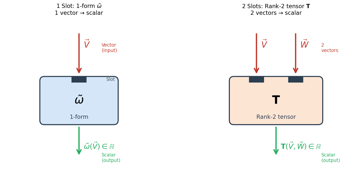
Fig. B.1: The slot machine picture of tensors. We view a tensor as "a machine with slots." Left — A 1-form (one slot) is a function that takes one vector and returns a scalar. Right — A rank-2 tensor (two slots) is a function that takes two vectors and returns a scalar. The precise meaning of "linear" is defined immediately after in the text.
Think of a tensor as "a machine with slots." Look at the left side of the figure—there's a box with one slot drawn. This is a 1-form: a linear function that takes one vector and produces a scalar. You learned this in the main text (Ch. 4). The right side of the figure shows a box with two slots—this is a rank-2 tensor that takes two vectors and produces a scalar. The key point is that it's independently linear in each argument placed in each slot—this property is called "multilinear." I'll explain the precise meaning of "independently linear" using equations shortly, but intuitively it means "if you fix one slot's content and double only the other, the output also doubles." The number of slots corresponds to the tensor's "rank."
⚪ Mei: I see, a 1-form is a machine with one slot, a rank-2 tensor is a machine with two slots... so as the rank increases, the number of slots increases?
🟡 Lina: Exactly. A rank-3 tensor has 3 slots, rank-4 has 4—rank = number of slots. Let's define this "machine with slots" mathematically. Before that, let me confirm two terms. First, "argument"—this is the value you input into a function. It corresponds to \(x\) in \(f(x)\). Next, "linear"—roughly speaking, it means "you can pull out scalar multiples and split apart sums." Here \(f\) is "a function that takes a vector as input and returns a real number (scalar)." In equation form, it means \(f(\alpha \vec{A}) = \alpha f(\vec{A})\) and \(f(\vec{A} + \vec{B}) = f(\vec{A}) + f(\vec{B})\) hold. For example, in 2 dimensions consider the function \(f(\vec{A}) = 2A^1 + 3A^2\) (twice the first component plus three times the second component). Then \(f(5\vec{A}) = 2(5A^1) + 3(5A^2) = 5(2A^1 + 3A^2) = 5f(\vec{A})\), so you can pull out the scalar multiple. "Linear in each argument" means that when there are multiple arguments, if you fix all others and vary just one, linearity holds for that one. I'll write the concrete equations shortly.
🟡 Lina: Using these two terms, the definition is: a function that takes \(N\) vectors as arguments, returns a real number, and is linear in each argument is defined to be a tensor.
⚪ Mei: By the way, "multilinear map" in the heading breaks down as "multi (multiple arguments) + linear (linear in each argument) + map," right? Does "map" mean the same as "function"?
🟡 Lina: Exactly. A "map" is "a correspondence that receives input and returns output"—it means the same as "function." The name is long, but the content is just what I explained.
🔵 Kai: Let me organize this. "A device where you put in \(N\) vectors and get out one real number, and moreover it's linear in each input"—that's the definition of a tensor? But earlier in B.7 we defined tensors as "elements of tensor product spaces." Are there two definitions?
🟡 Lina: Good question. This definition captures a tensor from a different angle than B.7—they look different, but they actually describe the same object. We'll formally show this in Section B.11. For now, think of it as "a tensor has two faces." And we write the "type" of this tensor as \((0, N)\), but—
🔵 Kai: What do the \(0\) and \(N\) in \((0, N)\) represent?
🟡 Lina: Good question. Recall the \((r, s)\) notation introduced in Section B.8—\(r\) is the number of upper (contravariant) indices, and \(s\) is the number of lower (covariant) indices. The \(T^r(V)\) defined in B.7 had \(r\) upper indices and 0 lower indices, so it's type \((r, 0)\). The current "function that eats vectors and returns a real number" has lower indices, so it becomes type \((0, N)\). Why a "function that eats vectors" has lower indices will be explained shortly. For example, a 1-form has one slot so it's type \((0, 1)\); a function with two slots like an inner product is type \((0, 2)\)—the number of slots corresponds to \(s\).
⚪ Mei: I see, so \(s\) represents the number of slots.
🟡 Lina: By the way, some textbooks use notation like \(\binom{0}{N}\), but since that's easily confused with binomial coefficients, we use \((r, s)\) in this book.
🔵 Kai: Wait, we were dealing with "contravariant tensors" with upper indices before, but now we're talking about lower indices?
🟡 Lina: Good question. Let me first organize the overall picture in a table, then explain "why lower indices."
| Type | Number of upper indices | Number of lower indices | Example |
|---|---|---|---|
| \((1, 0)\) | 1 | 0 | Vector \(A^i\) |
| \((2, 0)\) | 2 | 0 | \(S^{ij}\) from B.7 |
| \((0, 1)\) | 0 | 1 | 1-form \(f_i\) (introduced in Ch. 4 of the main text) |
| \((0, 2)\) | 0 | 2 | Metric tensor \(g_{ij}\) (formally introduced in Ch. 6 of the main text. Here we re-examine it from the multilinear map perspective. For now, understanding it as "coefficients that take two vectors and return an inner product" is OK) |
🔵 Kai: I learned about the metric tensor \(g_{ij}\) in the main text, but here it appears as "an example of a \((0,2)\) type tensor," right? I'm curious how it looks from the multilinear map perspective.
🟡 Lina: Good question. The formal definition of the metric tensor was already given in the main text (Ch. 6 and Ch. 7). The purpose here is to re-examine "the metric tensor being a representative example of a \((0,2)\) type tensor" from the multilinear map perspective. We'll revisit the \(g_{\alpha\beta}\) from Section B.6 (the coefficients for computing inner products) in the discussion that follows immediately, viewing it as "a bilinear function that takes two vectors and returns their inner product." Meanwhile, the current \((0, N)\) type tensor is "a tensor with \(N\) lower indices"—defined as a function that eats vectors and returns a real number. Tensors with lower indices are called covariant tensors.
🔵 Kai: Where does the name "covariant" come from?
🟡 Lina: Under coordinate transformations, the components transform in the same direction as the basis vectors, hence "covariant." This is the counterpart of "contravariant" meaning the opposite direction. The details are covered in Ch. 4 of the main text, but for now just remember "quantities with lower indices = covariant."
⚪ Mei: But why does a "function that eats vectors" have lower indices?
🟡 Lina: Think of it intuitively this way. In the summation convention we learned in B.6, upper and lower indices pair up for summation. Since vector components are upper \(A^i\), for a function's components to combine with them in a contraction, the function's components must be lower. Recall from Ch. 4 that the 1-form \(f_i\) had lower-index components—that was because it needed to be lower to "eat a vector \(A^i\) and return the scalar \(f_i A^i\)." For a rank-2 tensor, \(f_{ij} A^i B^j\) requires upper-lower pairs to sum. So "functions that eat vectors" naturally have lower indices.
🔵 Kai: I see, it's necessarily determined by the contraction rules. To "eat" a vector with upper-index components, the other side must be lower to form a pair—like puzzle pieces.
🟡 Lina: Yes, nice analogy. Upper and lower indices are different types of tensors, but the computational rules for tensor products and the approach to component representation are the same. The main text deals with general \((r, s)\) type tensors with mixed upper and lower indices, but here let's first grasp the idea of "multilinear maps" using covariant tensor examples.
🔵 Kai: What does "linear in each argument" mean?
🟡 Lina: Let's think about it with a function \(f(\vec{A}, \vec{B})\) that has 2 arguments. "Linear in the first argument" means that if you fix \(\vec{B}\) and vary only the first argument, it behaves like an ordinary linear function. In equations:
Linear in the first argument (fixing \(\vec{B}\)): $\(f(\alpha \vec{A} + \beta \vec{C},\; \vec{B}) = \alpha\,f(\vec{A}, \vec{B}) + \beta\,f(\vec{C}, \vec{B})\)$
Similarly, fixing \(\vec{A}\) and varying only the second argument is also linear:
Linear in the second argument (fixing \(\vec{A}\)): $\(f(\vec{A},\; \alpha \vec{B} + \beta \vec{C}) = \alpha\,f(\vec{A}, \vec{B}) + \beta\,f(\vec{A}, \vec{C})\)$
Let's verify with a concrete example. With the inner product \(f(\vec{A}, \vec{B}) = \vec{A} \cdot \vec{B}\), let \(\vec{A} = (1, 0)\), \(\vec{B} = (1, 1)\), \(\vec{C} = (0, 1)\). Setting \(\alpha = 2, \beta = 3\) and checking linearity in the second argument: the left side is \(f(\vec{A},\; 2\vec{B} + 3\vec{C}) = (1, 0) \cdot (2, 5) = 2\). The right side is \(2\,f(\vec{A}, \vec{B}) + 3\,f(\vec{A}, \vec{C}) = 2 \cdot 1 + 3 \cdot 0 = 2\). They indeed match.
A function that is linear in each argument when the other is fixed is called bilinear. In general, a function that is linear in all \(N\) arguments is called multilinear.
🔵 Kai: Wait, isn't the inner product \(\vec{A} \cdot \vec{B}\) "a function that takes two vectors and returns a real number"? That means it fits the current definition... is the inner product a type of tensor?
🟡 Lina: Good observation. Let's actually verify it. Recall the properties of the inner product from high school—\((\vec{A} + \vec{B}) \cdot \vec{C} = \vec{A} \cdot \vec{C} + \vec{B} \cdot \vec{C}\) and \((k\vec{A}) \cdot \vec{B} = k(\vec{A} \cdot \vec{B})\) hold. This is exactly "linear in the first argument." The same holds for the second argument, so the inner product is bilinear—it satisfies the conditions for a \((0, 2)\) type tensor.
🔵 Kai: Oh, the properties of the inner product from high school directly satisfy the "bilinear" conditions.
🟡 Lina: Exactly. Now let's see how it looks in component form. In the dummy index discussion of B.6, I mentioned "the coefficients \(g_{\alpha\beta}\) for computing the inner product." It's the same thing. In B.6 we used Greek letters \(\alpha, \beta\) with 4-dimensional spacetime in mind, but now since we're discussing general \(n\)-dimensional spaces, we'll write it with Latin letters \(i, j\) as \(g_{ij}\). Only the notation has changed—the content is the same. The index letters are merely indicators of "what dimension we're discussing."
⚪ Mei: Greek letters for 4-dimensional spacetime, Latin letters for general \(n\) dimensions—the same convention as the main text.
🟡 Lina: Right. Let me show why the inner product can be written as \(g_{ij} A^i B^j\)—let's check with a simple example. The inner product in ordinary 2-dimensional Euclidean space is \(\vec{A} \cdot \vec{B} = A^1 B^1 + A^2 B^2\). Fitting this into the form \(g_{ij} A^i B^j\), with \(g_{11} = 1, g_{22} = 1, g_{12} = g_{21} = 0\), we get \(g_{ij} A^i B^j = 1 \cdot A^1 B^1 + 0 \cdot A^1 B^2 + 0 \cdot A^2 B^1 + 1 \cdot A^2 B^2 = A^1 B^1 + A^2 B^2\), which matches.
🔵 Kai: I see. But in Euclidean space, \(g_{ij}\) is just the identity matrix, and you could just write \(A^1 B^1 + A^2 B^2\) without bothering with \(g_{ij}\). Why go through the trouble of using \(g_{ij}\)?
🟡 Lina: Good question. If you only consider Euclidean space, it's indeed unnecessary. But as we learned in the main text, in Minkowski spacetime \(g_{00} = -1\) puts a minus sign on the time component, and in curved spacetime \(g_{ij}\) varies from place to place. In other words, \(g_{ij}\) is needed to uniformly handle situations where "the rules for inner products differ depending on the space." For now, understand it as "a special case that becomes the identity matrix in Euclidean space."
⚪ Mei: So \(g_{ij}\) is "coefficients that specify the inner product computation rule component by component." In Euclidean space they're the same as the identity matrix components, but in general spaces that's not necessarily the case.
🟡 Lina: Exactly. In general spaces \(g_{ij}\) may not be the identity matrix, but the structure is the same. Now, I just said "the inner product satisfies the conditions for a \((0,2)\) type tensor." Let's actually verify this in the component form \(g_{ij} A^i B^j\)—that is, let's see that this expression is indeed linear in each argument. Fix \(\vec{A}\) and change the second argument to \(\alpha \vec{B} + \beta \vec{C}\). What we want to show is that \(g_{ij} A^i (\alpha B^j + \beta C^j) = \alpha\,g_{ij} A^i B^j + \beta\,g_{ij} A^i C^j\) holds—in other words, that the ordinary distributive law applies.
🔵 Kai: Isn't it obvious that the distributive law applies? You just expand normally...
🟡 Lina: Good question. The point is that the part \(g_{ij} A^i\) is "just a numerical value" that doesn't depend on \(\vec{B}\) or \(\vec{C}\). Let's verify concretely with \(n = 2\)—fixing \(j\) and computing \(g_{ij} A^i\): for \(j = 1\), \(g_{i1} A^i = g_{11} A^1 + g_{21} A^2\); for \(j = 2\), \(g_{i2} A^i = g_{12} A^1 + g_{22} A^2\)—these are numerical values determined solely by the components of \(\vec{A}\) and \(g_{ij}\), completely independent of how you choose \(\vec{B}\) or \(\vec{C}\). For example, in Euclidean space with \(\vec{A} = (3, 5)\): \(g_{i1} A^i = 1 \cdot 3 + 0 \cdot 5 = 3\), \(g_{i2} A^i = 0 \cdot 3 + 1 \cdot 5 = 5\)—these specific numerical values are fixed before you even decide on \(\vec{B}\) or \(\vec{C}\).
🔵 Kai: What does "fixing \(j\)" mean? Don't you sum over \(j\)?
🟡 Lina: Good question. In the expression \(g_{ij} A^i\), \(i\) appears as a pair in the upper (\(A^i\)) and lower (first index of \(g_{ij}\)), so it's a dummy index—you sum over \(i\). But \(j\) appears only once in \(g_{ij}\). An index that "remains without forming a pair" like this is called a free index—a term from Ch. 2 of the main text. A free index is not summed over; instead you consider it case by case—"when \(j = 1\)," "when \(j = 2\)." So \(g_{ij} A^i\) returns one numerical value for each value of \(j\)—when \(j = 1\) it's 3, when \(j = 2\) it's 5, and so on.
⚪ Mei: I see, \(g_{ij} A^i\) becomes one numerical value each time you fix \(j\). It's determined independently of \(\vec{B}\) or \(\vec{C}\).
🟡 Lina: Right. So when considering the expression \(g_{ij} A^i (\alpha B^j + \beta C^j)\), you fix \(j\) one at a time—looking at "when \(j = 1\)," "when \(j = 2\)" in sequence. For each fixed \(j\), \(g_{ij} A^i\) behaves as a fixed numerical value, so you can expand using the ordinary distributive law. Let me write it concretely for \(n = 2\). The \(j = 1\) term is \(g_{i1} A^i \cdot (\alpha B^1 + \beta C^1) = \alpha\,g_{i1} A^i B^1 + \beta\,g_{i1} A^i C^1\); similarly for \(j = 2\): \(\alpha\,g_{i2} A^i B^2 + \beta\,g_{i2} A^i C^2\).
🔵 Kai: Up to this point we were fixing \(j\) and doing case analysis. Do we sum over \(j\) at the end?
🟡 Lina: Exactly. Adding together the results for \(j = 1\) and \(j = 2\) gives \(\alpha\,g_{ij} A^i B^j + \beta\,g_{ij} A^i C^j\). In this final expression, \(j\) also appears as a pair—up in \(B^j\) and down in \(g_{ij}\)—so it's summed over as a dummy index.
⚪ Mei: So ultimately \(g(\vec{A},\; \alpha\vec{B} + \beta\vec{C}) = \alpha\,g(\vec{A}, \vec{B}) + \beta\,g(\vec{A}, \vec{C})\) holds—indeed linear in the second argument.
🟡 Lina: Exactly. Therefore the inner product \(g(\vec{A}, \vec{B}) = g_{ij} A^i B^j\) is indeed bilinear and is a representative example of a \((0, 2)\) type tensor. This is the metric tensor that appears in the main text.
⚪ Mei: I see, so the familiar operation of taking an inner product fits perfectly into the definition of a tensor.
🔵 Kai: Let me confirm. In the expression \(g_{ij} A^i B^j\), \(i\) is paired down in \(g_{ij}\) and up in \(A^i\) so you sum over it, and \(j\) is also paired down in \(g_{ij}\) and up in \(B^j\) so you sum over it... so it's a sum of \(n^2\) terms total, right?
🟡 Lina: Exactly. For \(n = 2\), it's the 4 terms \(g_{11}A^1 B^1 + g_{12}A^1 B^2 + g_{21}A^2 B^1 + g_{22}A^2 B^2\). Let me emphasize an important point here. In this discussion, to determine that "the inner product is bilinear and therefore a \((0,2)\) type tensor," we didn't use the specific values of the components \(g_{ij}\). The definition of a tensor itself is independent of components—it's determined solely by the property of "being a certain type of function." Components only appear once you choose a coordinate system. So how do you find the components? That's the topic of the next section, B.10.
🔵 Kai: ...So the tensor itself is a geometric object independent of coordinates, and the components are numerical values that only become determined once you choose a coordinate system? The same structure as with vectors. But for vectors there was the intuitive image of an "arrow"—what "shape" does a rank-2 or higher tensor have geometrically?
🟡 Lina: Good question, but it's difficult to represent rank-2 or higher tensors as a single picture. That's precisely why the abstract definition as "multilinear maps" is powerful—we characterize tensors not by their shape but by their behavior (what goes in, what comes out). And this way of thinking is key to naturally realizing the principle of general covariance—"physical laws are independent of coordinate systems"—in general relativity.
✅ Comprehension Check: When defining a tensor as a "multilinear map," what kind of function is a type \((0, 2)\) tensor? What is the advantage of this definition?
Answer
A type \((0, 2)\) tensor is a function that takes two vectors as arguments and returns a real number, and is linear in each argument (bilinear). The advantage of this definition is that no components or coordinate systems appear, allowing us to view tensors as geometric objects independent of coordinates.
B.10 Finding Tensor Components from "Multilinear Maps"
🟡 Lina: The components of a tensor viewed as a multilinear map are defined as the real numbers obtained by substituting basis vectors.
The components of a \((0, 2)\) type tensor \(f\) are
⚪ Mei: For the inner product \(g\) that appeared earlier, what does this definition give?
🟡 Lina: Good question. Let's verify with a concrete example from the main text. The Minkowski metric from Ch. 4 is exactly this kind of example. Since we're now discussing 4-dimensional spacetime, let me switch the indices to Greek letters \(\alpha, \beta\) (\(= 0, 1, 2, 3\))—the same notation as the main text. In flat spacetime, the components of the metric tensor \(g_{\alpha\beta}\) are constants, which we denote specifically as \(\eta_{\alpha\beta}\). Substituting the 4-dimensional spacetime basis \(e_0, e_1, e_2, e_3\):
Here \(g(e_\alpha, e_\beta)\) is "the inner product of basis vectors \(e_\alpha\) and \(e_\beta\) computed using the metric tensor \(g\)"—in other words, the metric tensor is the tool that defines the inner product. Under the sign convention \((-,+,+,+)\):
These are precisely the "components of the metric tensor." Once you know the components, you can calculate the value for any vectors.
🟡 Lina: Let me substitute \(\vec{A} = A^\alpha e_\alpha\) and \(\vec{B} = B^\beta e_\beta\). Note that we're using different dummy indices \(\alpha, \beta\) for expanding \(\vec{A}\) and \(\vec{B}\)—this is putting into practice the rule from Section B.6: "use different dummy indices for different sums."
First, use linearity in the first argument. Since \(\vec{A} = A^0 e_0 + A^1 e_1 + A^2 e_2 + A^3 e_3 = A^\alpha e_\alpha\), first split the sum:
Then pull out the scalar from each term:
🔵 Kai: Splitting the sum and then pulling out the scalars—you're using the linearity rules in two steps.
Next, applying linearity in the second argument in the same manner:
⚪ Mei: Just applying the same operation to the second argument as well. All the scalars come out cleanly.
Putting it together:
In this way, using multilinearity allows you to pull scalar coefficients out of the function one by one.
🔵 Kai: The spacetime indices are \(0, 1, 2, 3\), so expanding gives \(-A^0 B^0 + A^1 B^1 + A^2 B^2 + A^3 B^3\). That's exactly the inner product we saw in Ch. 5.
✅ Comprehension Check: How are the components \(f_{ij}\) of a tensor \(f\), viewed as a multilinear map, determined?
Answer
They are defined as the real numbers obtained by substituting basis vectors as arguments. That is, \(f_{ij} := f(e_i, e_j)\). Once the components are known, the value for any vectors can be computed using multilinearity as \(f(\vec{A}, \vec{B}) = A^i B^j f_{ij}\).
📝 Exercises:
- Computing components of a bilinear map → Problem M-2. Component Representation of Bilinear Maps, Evaluation of identity-type tensor → Problem M-8. Evaluation of the Identity Bilinear Form
B.11 Connecting the Two Approaches
🟡 Lina: So far, we've introduced tensors in two ways. Let me organize them in Table B.1 "Comparison of the two approaches to introducing tensors". In this section, we'll show that these two are actually the same thing.
🔵 Kai: I intuitively understand they're the same, but concretely how do you verify it? Can you "substitute" vectors into an element \(f_{ij}\,e_i \otimes e_j\) of the tensor product space?
🟡 Lina: Good question. That's actually the issue. Since \(e_i \otimes e_j\) is a product of vectors, it doesn't have a mechanism to "eat" vectors. As we learned in B.9, what can receive vectors as input and return real numbers are 1-forms. So if we prepare "partner" 1-forms corresponding to the basis vectors \(e_i\) and replace the tensor product space basis with \(\epsilon^i \otimes \epsilon^j\) (tensor products of 1-forms), then it can naturally eat vectors. These "partners" are the dual basis.
🔵 Kai: What does "dual" mean? I get the "partner" thing, but why is it called "dual"?
🟡 Lina: "Dual" means "paired." Vectors and 1-forms have an "eater/eaten" relationship—a vector gets eaten by a 1-form and returns a scalar; conversely, a 1-form gets eaten by a vector and returns a scalar. This symmetric paired relationship is called "dual." So "dual basis" means "a basis of 1-forms paired with the original basis."
Table B.1: Comparison of the two approaches to introducing tensors
| Approach | Core idea | Advantage |
|---|---|---|
| Tensor product space | Construct a space by lining up basis \(e_i \otimes e_j\) | Computational procedure is clear |
| Multilinear map | A function taking vectors as arguments and returning a real number | Definition independent of coordinates |
⚪ Mei: The two approaches feel like viewing the same object from different angles... are they actually the same thing?
🟡 Lina: Good intuition. Indeed, they can be shown to be mathematically identical. The reason we need to verify this is—if the two approaches are truly the same, then it's guaranteed that whether you "compute by arranging components" or "compute by substituting into a function," you always get the same answer. This lets you choose whichever method is more convenient for the situation. Let me state the goal first—we want to show that "substituting vectors into an element of the tensor product space gives the same result as computing via the multilinear map, \(f_{ij} A^i B^j\)." For this, we'll use the dual basis \(\epsilon^i\) that I introduced in response to Kai's question. By replacing the covariant tensor basis with \(\epsilon^i \otimes \epsilon^j\), we can naturally "eat" vectors, as we discussed.
🔵 Kai: Wait a moment. "Rebuilding the basis with 1-forms"—does that mean discarding the space we built with \(e_i \otimes e_j\)? Or are we building a new space?
🟡 Lina: Good question. We're not discarding anything. The contravariant tensor space \(T^2(V)\) remains as a space with basis \(e_i \otimes e_j\). What we want to do now is rewrite the space of covariant tensors—"functions that eat vectors"—in the language of tensor products. For that, we use the 1-form basis \(\epsilon^i\) to create the basis \(\epsilon^i \otimes \epsilon^j\). A reminder about 1-forms—they are "linear functions that take one vector and return one real number" (studied in detail in Ch. 4 of the main text).
🔵 Kai: Hmm... but why do we build the covariant one with 1-forms? Can't we use the vector basis \(e_i\)?
🟡 Lina: Covariant tensors are "functions that eat vectors," remember? So the basis elements themselves need to be able to eat vectors. \(e_1\) is just an arrow—it has no mechanism to receive \(\vec{A}\) and return a number. But 1-forms can return numbers—so we build the basis from 1-forms. Specifically, for the basis \(e_1, \ldots, e_n\) of \(V\), we define a set of 1-forms \(\epsilon^1, \ldots, \epsilon^n\). I'm using the Greek letter \(\epsilon\) (epsilon) because \(e^i\) would be confused with the exponential function \(e^x\). Some textbooks write \(\theta^i\). Pay attention to the index position—\(\epsilon^i\) has an upper index. It's opposite to the basis vectors \(e_i\) which have lower indices. As we saw in B.6, vectors have "upper-index components \(A^i\), lower-index basis \(e_i\)." 1-forms are the reverse: "lower-index components \(f_i\), upper-index basis \(\epsilon^i\)." Components and basis always have opposite index positions—this is the rule that ensures consistency with the summation convention.
⚪ Mei: I see, whether for vectors or 1-forms, there's a unified rule that "the indices of components and basis are always opposite."
🔵 Kai: So what exactly is \(\epsilon^i\) as a 1-form? What goes in and what comes out?
🟡 Lina: Good question. Earlier I said we want to "substitute vectors into elements of the tensor product space." For that, we need a tool that can extract each component of a vector one by one. We want \(\epsilon^i\) to play the role of "a device that extracts only the \(i\)-th component." Think about it concretely—if you have a vector \(\vec{A} = 3e_1 + 5e_2\), you'd want "a device that extracts just the first component, 3" and "a device that extracts just the second component, 5." \(\epsilon^1\) plays the former role, \(\epsilon^2\) the latter. "Extracting the first component" means that inputting \(e_1\) returns 1, and inputting \(e_2\) returns 0—then \(\epsilon^1(3e_1 + 5e_2) = 3 \cdot 1 + 5 \cdot 0 = 3\), leaving only the first component. In general, we want each one to "return 1 for its own number and 0 for all others." Writing this as an equation:
🔵 Kai: \(\delta^i{}_j\)... ah, that's the Kronecker delta, right? It appeared in Ch. 6. It returns 1 when \(i = j\) and 0 when \(i \neq j\).
🟡 Lina: Yes, good memory. Here we write the indices split up-down as \(\delta^i{}_j\), but the numerical value is the same.
🔵 Kai: If the numerical value is the same, why bother splitting them up and down? Isn't \(\delta_{ij}\) fine?
🟡 Lina: Good question. The reason is consistency with the summation convention. Look at the left side—in \(\epsilon^i(e_j)\), \(\epsilon^i\) has an upper index and \(e_j\) has a lower index. If the right side also has the same index arrangement, the "sum over upper-lower pairs" rule works seamlessly in later calculations. Numerically, \(\delta^i{}_j\), \(\delta_{ij}\), and \(\delta^{ij}\) are all the same (1 if \(i = j\), 0 otherwise), so at this stage think of it as "a notational convention."
⚪ Mei: Essentially it's the same value as the \((i, j)\) entry of the identity matrix, but keeping the index positions aligned prevents confusion in later calculations.
🟡 Lina: Exactly. So each \(\epsilon^i\) is a 1-form that "extracts only the \(i\)-th basis component." By the way, some textbooks write the dual basis as \(e^i\), but since that's confusable with the exponential \(e^x\), we use \(\epsilon^i\) in this book.
🔵 Kai: A 1-form is a function that eats a vector and returns a real number, right? So \(\epsilon^i\) means "returns 1 when you input \(e_i\), returns 0 when you input any other basis vector"?
🟡 Lina: Exactly. Let's verify with a concrete example. Applying \(\epsilon^1\) to \(\vec{A} = 3e_1 + 5e_2\): \(\epsilon^1(\vec{A}) = \epsilon^1(3e_1 + 5e_2) = 3\,\epsilon^1(e_1) + 5\,\epsilon^1(e_2) = 3 \cdot 1 + 5 \cdot 0 = 3\). It extracts just the first component.
⚪ Mei: I see, \(\epsilon^i\) is like "a device that reads off the \(i\)-th component."
🟡 Lina: Right. And when we build a space with the tensor products \(\epsilon^i \otimes \epsilon^j\) of these dual basis elements as the basis, we can define the operation of "substituting" vectors \(\vec{A}, \vec{B}\) into an element \(f = f_{ij}\,\epsilon^i \otimes \epsilon^j\) of that space.
🔵 Kai: "Substituting" vectors into an element of the tensor product space—concretely how do you do that?
🟡 Lina: The definition rule is natural: \((\epsilon^i \otimes \epsilon^j)(\vec{A}, \vec{B}) := \epsilon^i(\vec{A})\,\epsilon^j(\vec{B})\)—the left side of the tensor product handles the first argument, and the right side handles the second argument.
🔵 Kai: The left \(\epsilon^i\) eats \(\vec{A}\), and the right \(\epsilon^j\) eats \(\vec{B}\)... it's like inserting one into each slot of a machine with two slots.
🟡 Lina: Exactly. Generalizing the concrete example from before, \(\epsilon^i\) is a 1-form, hence a linear function. Recall the rule for linear functions—\(\epsilon^i(\alpha \vec{u} + \beta \vec{v}) = \alpha\,\epsilon^i(\vec{u}) + \beta\,\epsilon^i(\vec{v})\) holds. Let me substitute \(\vec{A} = A^k e_k\) (summation convention over \(k\)). Note that I'm using \(k\) rather than \(i\) as the dummy index because the upper index \(i\) of \(\epsilon^i\) is already in use—this is practicing the rule from Section B.6: "use different dummy indices for different sums." Expanding: \(\vec{A} = A^1 e_1 + A^2 e_2 + \cdots + A^n e_n\), so using linearity repeatedly to split into individual terms: \(\epsilon^i(\vec{A}) = \epsilon^i(A^1 e_1 + A^2 e_2 + \cdots) = A^1\,\epsilon^i(e_1) + A^2\,\epsilon^i(e_2) + \cdots = A^k\,\epsilon^i(e_k)\). The scalar \(A^k\) can be pulled out of the function by the linearity rule itself. And since \(\epsilon^i(e_k) = \delta^i{}_k\), we get \(A^k\,\delta^i{}_k\).
🔵 Kai: Ah, that's the Kronecker delta discussion from earlier. When you sum over \(k\), only the \(k = i\) term survives...
🟡 Lina: Exactly. Let me supplement the final step. Since \(\delta^i{}_k\) is 1 only when \(i = k\) and 0 otherwise, summing over \(k\) leaves only the \(k = i\) term. That is, \(A^k\,\delta^i{}_k = A^1 \cdot 0 + \cdots + A^i \cdot 1 + \cdots + A^n \cdot 0 = A^i\). This is the "index-replacing" function of the Kronecker delta.
🔵 Kai: Let me confirm. In \(A^k \delta^i{}_k\) when summing over \(k\), \(i\) is fixed, right? For example, if \(i = 2\), then \(A^1 \cdot \delta^2{}_1 + A^2 \cdot \delta^2{}_2 + \cdots = 0 + A^2 + 0 + \cdots = A^2\)?
🟡 Lina: Exactly. \(i\) is a free index so it's fixed, and only \(k\) runs as a dummy index. If \(i = 2\), only the \(k = 2\) term survives giving \(A^2\). The same mechanism gives \(A^i\) for general \(i\).
⚪ Mei: So \(\epsilon^i(\vec{A}) = A^i\). \(\epsilon^i\) simply returns the \(i\)-th component of the vector.
🟡 Lina: Correct. Similarly \(\epsilon^j(\vec{B}) = B^j\), so putting it all together:
So it behaves as "a function that takes two vectors and outputs a real number." Conversely, substituting basis vectors into a multilinear map yields the components. Mathematically, these two spaces are isomorphic.
🔵 Kai: "Isomorphic"... does that mean they have the same shape?
🟡 Lina: Roughly speaking, yes. More precisely, it means "they look different, but have exactly the same structure for addition and scalar multiplication." As a familiar example, representing points on a 2-dimensional plane by "coordinates \((x, y)\)" versus "arrows (vectors)"—they look different, but the rules for addition and scalar multiplication are the same, so either way of computing gives the same answer. The same holds for tensors: if the components \(f_{ij}\) are the same, computing via the tensor product space approach or the multilinear map approach always yields the same numerical values.
🔵 Kai: Ah, it's like the relationship between coordinates and vectors. Only the representation differs while the content is the same... but does it really always give the same answer? Isn't it possible that they just happened to agree in this example?
🟡 Lina: Good question. What guarantees it's not "just a coincidence" is the mathematical concept of "isomorphism." It means "there exists a one-to-one correspondence between the two spaces that doesn't destroy the structure of addition and scalar multiplication." "Doesn't destroy the structure" means that, for example, whether you add two elements first then apply the correspondence, or apply the correspondence to each then add, you get the same result.
🔵 Kai: Hmm, that's abstract and a bit hard to visualize. What does it mean concretely?
🟡 Lina: Let's look concretely. Adding elements \(f_{ij}\,\epsilon^i \otimes \epsilon^j\) and another \((0,2)\) type tensor \(h_{ij}\,\epsilon^i \otimes \epsilon^j\) in the tensor product space gives \((f_{ij} + h_{ij})\,\epsilon^i \otimes \epsilon^j\). On the other hand, viewing each as a multilinear map and then adding: \((f + h)(\vec{A}, \vec{B}) = f_{ij} A^i B^j + h_{ij} A^i B^j = (f_{ij} + h_{ij}) A^i B^j\)—the same components \(f_{ij} + h_{ij}\) appear. So "add first then apply the correspondence" and "apply the correspondence then add" coincide—hence the two spaces have the same structure, i.e., they're isomorphic.
⚪ Mei: I see, since the components match regardless of which approach you use to compute, the results are always the same.
🔵 Kai: Because the same components come out regardless of the order of addition, you can say they're "structurally the same." So whether you compute with components or substitute into functions, the final numerical values absolutely agree—therefore you can use whichever method... Ah, but wasn't that discussion about covariant tensors? Is there a similar perspective for contravariant tensors?
🟡 Lina: Good question. The same kind of correspondence holds for contravariant tensors. Symmetric to how covariant tensors are "functions that eat vectors," contravariant tensors can be viewed as "functions that eat 1-forms and return real numbers." Only the roles of upper and lower indices are swapped. For example, when a 1-form \(f = f_j \epsilon^j\) acts on a vector \(\vec{A} = A^i e_i\), it gives the scalar \(f(\vec{A}) = f_i A^i\). This corresponds to viewing a vector (type \((1,0)\)) as "a function that eats one 1-form and returns a real number." The details are covered in the main text, so for now just hold onto the image.
🔵 Kai: I see... covariant "eats vectors," contravariant "eats 1-forms"—only the up-down is swapped but the structure is the same.
🟡 Lina: In practice, it's best to use the tensor product space approach when computing (line up components and do addition/scalar multiplication), and use the multilinear map approach for understanding concepts (geometric objects independent of coordinates).
⚪ Mei: Computation with components, concepts with maps—using tools according to the situation.
📝 Exercises:
- Decomposition into symmetric and antisymmetric tensors → Problem A-1. Symmetric and Antisymmetric Decomposition, Dual space and tensor products → Problem A-2. Tensor Representation via Dual Spaces
Preview of Next Chapter
🟡 Lina: In the next chapter, Appendix C, we extend the action principle for particles to fields. We'll introduce the concept of Lagrangian density, derive the Euler–Lagrange equations for fields, learn how to write the action for fields in curved spacetime, and show the path toward the Einstein–Hilbert action.
Exercises
📝 Exercises:
- Expanding tensor products → Problem B-1. Basics of the Tensor Product \(S \otimes T\)
- Verifying non-commutativity → Problem B-2. Non-commutativity of the Tensor Product
- Addition and scalar multiplication in tensor product spaces → Problem B-3. Linear Combinations of Tensors
- Necessary and sufficient condition for decomposable tensors → Problem M-1. Condition for Decomposable Tensors
- Concrete example of indecomposability → Problem M-7. Non-decomposability of Antisymmetric Tensors
- Dimensions of tensor product spaces → Problem B-4. Dimensions of Tensor Spaces
- Expanding summation convention → Problem B-5. Expansion of Einstein Summation
- Convention violations in summation notation → Problem B-6. Violations of the Einstein Convention
- Reconstruction from components → Problem B-7. Reconstructing a Tensor from Components
- Tensor products of different ranks → Problem B-8. Tensor Product of Rank 1 and Rank 2 Tensors
- Proof of rank additivity → Problem M-3. Rank Addition via Tensor Product
- Rank-0 tensors and scalars → Problem M-4. \(T^0(V)\) and Scalars
- Tensor product computation practice → Problem M-5. Simple \(S \otimes T\) Expansion
- Dimensions in 3D → Problem M-6. Dimension of Tensor Spaces in 3-Dimensional Space
- Computing components of a bilinear map → Problem M-2. Component Representation of Bilinear Maps
- Evaluation of identity-type tensor → Problem M-8. Evaluation of the Identity Bilinear Form
- Decomposition into symmetric and antisymmetric tensors → Problem A-1. Symmetric and Antisymmetric Decomposition
- Dual space and tensor products → Problem A-2. Tensor Representation via Dual Spaces
References
- Toshimasa Ishii, Understanding General Relativity Step by Step with Equations, Chapters 6–7 (Fundamentals of Tensors / Tensor Fields in Rectilinear Coordinates)
- B. Schutz, A First Course in General Relativity, 3rd ed., Chapter 3 (Tensor Analysis in Special Relativity)
- T. Lancaster & S. J. Blundell, General Relativity for the Gifted Amateur, Chapter 2 (Vectors and Tensors)
Feedback on this page
Let us know if something was unclear, incorrect, or could be improved.