Chapter 6: Time Evolution of Two-State Systems — The Ammonia Maser and Quantum Oscillations
Story so far:
In Ch. 4, we learned Feynman's three laws—"the probability is the absolute square of the amplitude," "add amplitudes for each path," and "multiply amplitudes for successive processes." In Ch. 5, through the Stern-Gerlach experiment, we saw that the state of a spin-1/2 particle can be written as a superposition of two basis states, and that the coefficients (probability amplitudes) behave like complex vector components. The "skeleton" of state space is in place—but time has not yet entered the picture.
Goals of this chapter
- Write down a differential equation describing how probability amplitudes change with time for a two-state system, and by finding the eigenvalues and eigenvectors of the Hamiltonian matrix, derive stationary states and quantum oscillations (Rabi oscillations)
- As a concrete example, treat the inversion motion of the ammonia molecule NH₃ and the operating principle of the ammonia maser, gaining a visceral understanding of "why the Hamiltonian is central to quantum mechanics"
6.1 The Fundamental Equation of Time Evolution — What Rules Govern How Amplitudes Change in Time?
🟡 Lina: In the previous chapters, we learned that the state of a two-state system can be written as
Here \(C_1 = \langle 1|\psi\rangle\), \(C_2 = \langle 2|\psi\rangle\) are complex probability amplitudes satisfying \(|C_1|^2 + |C_2|^2 = 1\).
🔵 Kai: Yes. But this is just a "snapshot at a particular moment," right? How do \(C_1\) and \(C_2\) change as time passes?
🟡 Lina: Great question. That's precisely the theme of this chapter. In classical mechanics, Newton's equation of motion \(F = ma\) determined how an object's position changes in time. Quantum mechanics also has an equation that determines how amplitudes change in time.
🔵 Kai: So it's the quantum mechanics version of the "equation of motion."
🟡 Lina: Exactly. Here I'll present it as a given—that is, as a "fundamental postulate consistent with experimental facts"—but there are reasons for this form. There are three requirements.
First, the equation must be linear. This is to preserve the superposition principle.
Second, probability must be conserved. \(|C_1|^2 + |C_2|^2 = 1\) must hold at all times.
Third, the equation must be first order.
🔵 Kai: Why first order? Newton's equation of motion was second order, right?
🟡 Lina: Good comparison. Because Newton's equation is second order, you needed to specify both the position and the velocity as initial conditions. But in quantum mechanics, the state vector \(|\psi\rangle\)—that is, the set of amplitudes \(C_1(t), C_2(t)\)—contains all information about the system. For our ammonia molecule, if you know the two complex numbers \(C_1(t)\) and \(C_2(t)\), then "the probability of the nitrogen being above," "the probability of being below," and even how things will change in the future—everything is determined.
🔵 Kai: Hmm, I don't quite see why "contains all information" implies "first order is sufficient"...
🟡 Lina: Think of it this way. In classical mechanics, knowing just the ball's position \(x\) isn't enough to determine its future motion—you also need the velocity \(v\), otherwise you can't tell whether it's stationary or moving. That's why Newton's equation is second order, requiring both \(x\) and \(v\) as initial conditions.
But in quantum mechanics, the set of amplitudes \(C_1, C_2\) is the complete description of the system—meaning information equivalent to both "position" and "velocity" is all contained within them. If the equation were second order, you'd need to specify \(dC_1/dt|_0\), \(dC_2/dt|_0\) in addition to \(C_1(0)\), \(C_2(0)\) for the solution to be unique. That would mean "amplitudes alone aren't enough information," contradicting the hypothesis that "amplitudes provide a complete description." Therefore, the equation must be first order.
In other words, if you accept the hypothesis that "amplitudes are the complete description of the system," the first-order nature of the equation follows logically. And this hypothesis itself should be accepted as a fundamental principle consistent with experimental facts.
🔵 Kai: So "amplitudes alone are complete" is something we just have to accept as given for now.
🟡 Lina: Right. Whether this hypothesis is correct is judged by whether the predictions derived from it agree with experiment—and in this very chapter, predicting the oscillation frequency of ammonia molecules and comparing with experiment is precisely that verification. Now, the most general linear differential equation satisfying these three requirements takes the following form:
Why is there no constant term on the right side (a term not proportional to \(C_1\) or \(C_2\))? Because if there were a constant term, then even when \(C_1 = C_2 = 0\) (the state of nothing), amplitude would spontaneously appear—this would mean "probability springing from nothing," which is physically unreasonable.
🔵 Kai: Whoa, differential equations all of a sudden... \(\hbar\) is the reduced Planck constant we saw before, right? The \(i\) on the left side is the imaginary unit. But what are \(H_{11}\) and \(H_{12}\) on the right side? What do the subscript numbers mean?
🟡 Lina: Those are the components of the Hamiltonian matrix. The meaning of the subscripts is: the first subscript \(i\) in \(H_{ij}\) denotes the "row" (which amplitude's equation is on the left side), and the second subscript \(j\) denotes the "column" (which amplitude it multiplies on the right side). For example, \(H_{12}\) is "the coefficient of \(C_2\) (column 2) appearing in the equation for \(C_1\) (row 1)." These are quantities with dimensions of energy, and in general are complex numbers. I'll explain the physical meaning in detail in the next section, but for now just think of them as "constants related to energy." First, I want you to appreciate the "form" of the equation.
⚪ Mei: The left side is "the rate of change of \(C_1\) in time" multiplied by \(i\hbar\). The right side is a linear combination of \(C_1\) and \(C_2\). In other words, the change in one amplitude depends on the values of both amplitudes.
🟡 Lina: Exactly. \(C_1\) and \(C_2\) change in time while "influencing each other"—this is the equation of motion for a quantum two-state system.
🔵 Kai: What would equations (6.2a) and (6.2b) look like written as a matrix?
🟡 Lina: Good instinct. It can be written as:
The \(2 \times 2\) matrix on the right side is the Hamiltonian matrix \(H\).
✅ Comprehension Check: The \(i\hbar\) multiplying the left side of equation (6.3) is a constant. If \(H_{12} = H_{21} = 0\), what would happen to \(C_1\) and \(C_2\)? (Hint: the coupled equations "decouple.")
Answer
If \(H_{12} = H_{21} = 0\), equation (6.2a) becomes \(i\hbar\,dC_1/dt = H_{11}\,C_1\), independent of \(C_2\). Similarly, equation (6.2b) becomes \(i\hbar\,dC_2/dt = H_{22}\,C_2\). So \(C_1\) and \(C_2\) evolve independently in time. The off-diagonal elements \(H_{12}\), \(H_{21}\) play the role of "coupling the two states."
6.2 Introducing the Hamiltonian Matrix — A Matrix Representing Energy
🔵 Kai: So what does the Hamiltonian matrix actually represent?
🟡 Lina: In a word, it's a matrix that contains all information about the system's energy. The name comes from Hamilton, who in classical mechanics called the function representing the total energy of a system (kinetic energy + potential energy) the Hamiltonian.
🔵 Kai: So it's the "quantum version" of the classical total energy?
🟡 Lina: You can think of it that way. However, in quantum mechanics, the energy becomes not "a single number" but "a matrix." The reason is that since there are two states, you need to describe not only "the energy of state \(|1\rangle\)" and "the energy of state \(|2\rangle\)" but also "the coupling between states \(|1\rangle\) and \(|2\rangle\)."
⚪ Mei: I see—a single number isn't enough, and you need as many "slots" as there are states, so it becomes a matrix.
🟡 Lina: Right. Let me organize the meaning of each component:
Table 6.1: Physical meaning of each component of the Hamiltonian matrix
| Component | Meaning |
|---|---|
| \(H_{11}\) | The "self-energy" when in state \(\|1\rangle\) |
| \(H_{22}\) | The "self-energy" when in state \(\|2\rangle\) |
| \(H_{12}\) | The "strength of transition amplitude" from state \(\|2\rangle\) to state \(\|1\rangle\) (first subscript is "destination," second is "origin") |
| \(H_{21}\) | The "strength of transition amplitude" from state \(\|1\rangle\) to state \(\|2\rangle\) (similarly, 2 is destination, 1 is origin) |
🔵 Kai: So diagonal elements are energies, and off-diagonal elements are the "connections" between states.
🟡 Lina: Right. And the Hamiltonian matrix has one important property: Hermiticity (the Hermitian property):
This means "the matrix obtained by taking the complex conjugate of each element and then swapping rows and columns equals the original matrix." Specifically, the complex conjugate of \(H_{12}\) equals \(H_{21}\). For diagonal elements \(H_{11}\), \(H_{22}\), we have \(H_{11}^* = H_{11}\), \(H_{22}^* = H_{22}\), so diagonal elements are real.
🔵 Kai: Why must it be Hermitian?
🟡 Lina: Conservation of probability is the reason. For \(|C_1|^2 + |C_2|^2 = 1\) to hold at all times, the Hamiltonian matrix must be Hermitian. Let's take a brief look. If we require \(d(|C_1|^2 + |C_2|^2)/dt = 0\) and use equation (6.2) to compute the left side, the condition \(H_{12} = H_{21}^*\) emerges—this is precisely Hermiticity.
🔵 Kai: The complex conjugate part is a little concerning...
🟡 Lina: Just a hint for the calculation: since \(|C_1|^2 = C_1^* C_1\), when you differentiate you use the product rule: \(d|C_1|^2/dt = (dC_1^*/dt)C_1 + C_1^*(dC_1/dt)\). From equation (6.2a), \(dC_1/dt = (H_{11}C_1 + H_{12}C_2)/(i\hbar)\). To find \(dC_1^*/dt\), take the complex conjugate of both sides of equation (6.2a)—note that taking the complex conjugate changes \(i\) to \(-i\), so the left side becomes \(-i\hbar\,dC_1^*/dt\) and the right side becomes \(H_{11}^*\,C_1^* + H_{12}^*\,C_2^*\). Substituting these in and simplifying yields \(H_{12} = H_{21}^*\). Check the detailed calculation in the exercise (Problem B-1. Calculation of the Phase Factor for a Stationary State).
📝 Exercises:
- From \(d(|C_1|^2 + |C_2|^2)/dt = 0\) and equation (6.2), derive the Hermiticity condition \(H_{12} = H_{21}^*\). → Problem B-1. Calculation of the Phase Factor for a Stationary State
Intuitively, this corresponds to "energy should be real."
⚪ Mei: So the physical requirement that "energy should be real" is expressed as a mathematical property of the matrix (Hermiticity).
🟡 Lina: Good catch. The eigenvalue story is coming up very soon.
Why \(i\hbar\) Appears on the Left Side
🔵 Kai: One thing that bothers me—what's the purpose of \(i\hbar\) on the left side of equation (6.2)? Couldn't we just write \(dC_1/dt = (\text{something}) \times C_1 + \cdots\)?
🟡 Lina: Good question. If there were no \(i\), that is,
then when \(H_{11}\) is real, \(C_1\) would exponentially grow or decay while remaining real. This would violate probability conservation. The presence of \(i\) makes the solution oscillatory (the phase rotates), keeping \(|C_1|^2\) constant.
🔵 Kai: I see. So \(i\) plays the role of producing "rotation" rather than "growth or decay."
🟡 Lina: Exactly. And \(\hbar\) is there to match units. Since \(C\) is a probability amplitude and dimensionless, \(dC/dt\) has dimensions of \([\text{time}]^{-1}\). The dimensions of \(\hbar\) are \([\text{energy} \times \text{time}]\), so the left side \(i\hbar\,dC/dt\) has dimensions \([\text{energy} \times \text{time}] \times [\text{time}]^{-1} = [\text{energy}]\). On the right side, \(H_{ij} C_j\) also has dimensions of energy since \(H_{ij}\) has energy dimensions, so everything is consistent.
🔵 Kai: I see. So to summarize: \(i\) is "to conserve probability (to produce oscillations)," \(\hbar\) is "to match dimensions," and the right side being a linear combination of \(C_1\) and \(C_2\) is "to preserve the superposition principle"—the three requirements correspond to each part of the equation.
🟡 Lina: Exactly. Well summarized.
✅ Comprehension Check: What physical requirement does the Hermiticity \(H_{ij}^* = H_{ji}\) of the Hamiltonian matrix come from?
Answer
It comes from the requirement that the total probability \(|C_1|^2 + |C_2|^2 = 1\) does not change in time. Hermiticity also guarantees that the eigenvalues (energies) of the Hamiltonian are real.
6.3 The Two-State Model of the Ammonia Molecule
🟡 Lina: Now let's move on to a concrete example: the ammonia molecule NH₃.
🔵 Kai: Ammonia—the one with the pungent smell...?
🟡 Lina: That's right. It's a molecule consisting of 1 nitrogen atom (N) and 3 hydrogen atoms (H), shaped like a pyramid. The three hydrogen atoms form a triangular plane, and the nitrogen atom sits slightly above that plane (Fig. 6.1 "Structure of the ammonia molecule").
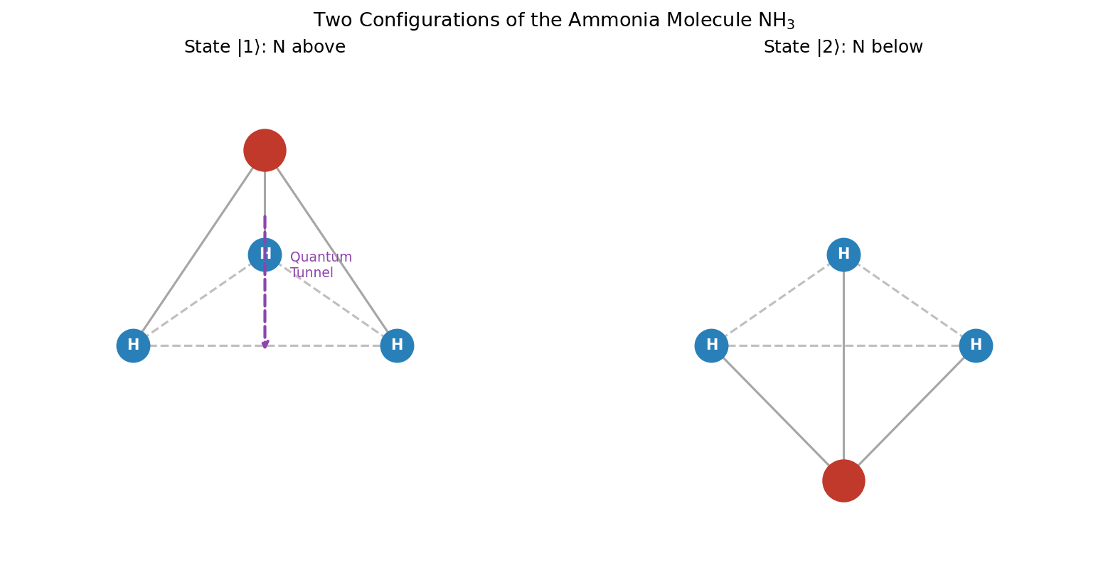
Fig. 6.1: Structure of the ammonia molecule. Structure of the ammonia molecule NH₃. The nitrogen atom (N) is located above or below the plane formed by the three hydrogen atoms (H).
🔵 Kai: A pyramid shape... so there are two possible configurations depending on whether nitrogen is "above" or "below"!
🟡 Lina: Exactly. Here we make a bold approximation. We fix all the molecule's rotation, vibration, and translational motion, so that the only remaining degree of freedom is which side of the hydrogen plane the nitrogen atom is on. This gives us a two-state system.
- State \(|1\rangle\): Configuration with nitrogen "above" the plane
- State \(|2\rangle\): Configuration with nitrogen "below" the plane
⚪ Mei: The actual molecule has many more degrees of freedom, but we "freeze" them and focus only on the nitrogen's up-down position—an approximation.
🟡 Lina: Right. This approximation is justified when the energy scale of the other degrees of freedom is much larger than the energy scale of the nitrogen inversion motion. Indeed, electronic excitation energies are several eV, molecular vibrations are around 0.1 eV, whereas the energy involved in nitrogen inversion is on the order of \(10^{-4}\) eV—orders of magnitude smaller.
Determining the Hamiltonian
🟡 Lina: Now let's determine the Hamiltonian matrix for this two-state system. The key is symmetry.
🔵 Kai: Symmetry?
🟡 Lina: Look at Fig. 6.1 "Structure of the ammonia molecule" again. Consider the operation of flipping the ammonia molecule upside down. The configuration with nitrogen "above" swaps exactly into the configuration with nitrogen "below." In other words, states \(|1\rangle\) and \(|2\rangle\) are physically completely equivalent.
⚪ Mei: That means \(H_{11} = H_{22}\). Both configurations have the same "self-energy."
🟡 Lina: Right. Let's write this common value as \(E_0\):
✅ Comprehension Check: Why is \(H_{11} = H_{22}\) in the Hamiltonian of the ammonia molecule? What is the physical reason?
Answer
When the ammonia molecule is flipped upside down, the configuration with nitrogen "above" and the one with nitrogen "below" are interchanged. Since the molecule is physically equivalent under this operation, the "self-energies" of the two configurations must have the same value \(E_0\).
Next, the off-diagonal elements. The nitrogen atom "tunnels through" the plane of hydrogen atoms to reach the other side—in classical mechanics, this would be impossible if the energy is insufficient. But in quantum mechanics, quantum tunneling occurs. In classical mechanics, if the energy is lower than the barrier height, passage is absolutely impossible, but in quantum mechanics the probability amplitude for "slipping through" to the other side is not zero.
🔵 Kai: Tunneling! In Ch. 3, with the double slit, there was discussion of "classically impossible paths" too.
🟡 Lina: Good connection. Let's write this "tunneling through" amplitude as \(-A\) (with \(A > 0\)). The minus sign is conventional—it makes the calculations neater later. By symmetry, \(H_{12} = H_{21}\):
⚪ Mei: The Hermiticity condition \(H_{12}^* = H_{21}\) is also satisfied. If \(A\) is real, then \((-A)^* = -A = H_{21}\).
🟡 Lina: In summary, the Hamiltonian matrix for the ammonia molecule is:
🔵 Kai: That's simple. But how is the value of \(A\) determined?
🟡 Lina: \(A\) is related to the probability amplitude for the nitrogen atom to quantum tunnel through the potential barrier, and in principle can be calculated from the barrier height and width, but in practice we use values measured experimentally. For the ammonia molecule, the frequency corresponding to \(2A\) is known to be about 24,000 MHz (microwave radiation with a wavelength of about 1.25 cm).
🔵 Kai: So it's in the microwave range.
📝 Exercises:
- Given \(2A = hf\) with \(f = 24{,}000\) MHz, find \(A\) in units of eV. → Problem B-2. Energy Calculation of Tunnel Splitting
6.4 Eigenvalues and Eigenvectors — Finding Stationary States
🟡 Lina: Now that the Hamiltonian matrix (6.7) is determined, let's solve equation (6.2). First, we'll look for stationary states—special states whose "character" doesn't change as time passes.
🔵 Kai: What does "character doesn't change" mean?
🟡 Lina: It means states where the ratio \(C_1 : C_2\) of the amplitudes remains constant in time. Since equation (6.2) has the form "the derivative is proportional to the original function," it's natural to try an exponential solution—the same idea as the solution \(e^{kx}\) to \(dy/dx = ky\) that you learned in high school. Specifically:
Here \(a_1\), \(a_2\) are time-independent constants, and \(E\) is a constant (with dimensions of energy).
⚪ Mei: Since both amplitudes oscillate at the same frequency \(E/\hbar\), the ratio \(C_1/C_2 = a_1/a_2\) is time-independent.
🟡 Lina: Right. Let's substitute equation (6.8) into equation (6.2). The left side is:
The right side is:
Dividing both sides by \(e^{-iEt/\hbar}\):
Similarly from equation (6.2b):
🔵 Kai: Oh, the differential equation disappeared and became just a system of algebraic equations!
🟡 Lina: Right. Writing it in matrix form:
🟡 Lina: In linear algebra, this is called an eigenvalue problem. When you multiply the matrix \(H\) by the vector \(\begin{pmatrix} a_1 \\ a_2 \end{pmatrix}\), you get a scalar multiple \(E\) times the original vector—we're looking for such special vectors and values of \(E\). \(E\) is called the eigenvalue, and \(\begin{pmatrix} a_1 \\ a_2 \end{pmatrix}\) is called the eigenvector. "Eigen" is German for "characteristic of that thing"—meaning "special values and vectors that belong uniquely to that matrix."
🔵 Kai: Why are vectors that become "scalar multiples" special? How is this different from an ordinary system of equations?
🟡 Lina: Let me answer from two perspectives. First, the difference from ordinary systems of equations. The systems you solved in high school had the form "\(2x + 3y = 5\), \(x - y = 1\)"—the right side is a fixed constant, and you find one set of values for the unknowns \(x, y\). But in an eigenvalue problem, the "right side is a scalar multiple of the unknowns themselves"—meaning the scalar \(E\) itself is also unknown, and you're looking for \(E\) and the vector simultaneously. Moreover, there are generally multiple solution sets—in our case, two.
🔵 Kai: I see, \(E\) is part of the unknowns too... So there are more unknowns to solve for than usual.
🟡 Lina: Next, the geometric picture. In general, when you multiply a matrix times a vector, both the direction and length of the vector change. But eigenvectors are special—when you multiply them by the matrix, their direction doesn't change—only the length (scalar multiple) changes. For example, \(\begin{pmatrix} 2 & 1 \\ 0 & 3 \end{pmatrix}\begin{pmatrix} 1 \\ 0 \end{pmatrix} = \begin{pmatrix} 2 \\ 0 \end{pmatrix} = 2\begin{pmatrix} 1 \\ 0 \end{pmatrix}\)—the vector \(\begin{pmatrix} 1 \\ 0 \end{pmatrix}\) keeps its direction unchanged by the matrix and only gets multiplied by 2. Finding eigenvectors means finding "directions that are stable under the matrix's action."
⚪ Mei: "Direction unchanged under the matrix's action = character unchanged as time passes"—the mathematics and physics correspond beautifully.
🟡 Lina: And the physical meaning. Remember: we were looking for states where the ratio \(C_1 : C_2\) remains constant in time. In equation (6.8), assuming the common factor \(e^{-iEt/\hbar}\) was precisely for this purpose. If we find solutions to the eigenvalue problem, they correspond to stationary states—states with definite energy. The eigenvalue \(E\) is the energy of that stationary state.
Calculating the Eigenvalues
🟡 Lina: Let's rewrite equation (6.10). First, let me introduce one symbol. \(\mathbb{1} = \begin{pmatrix} 1 & 0 \\ 0 & 1 \end{pmatrix}\) is called the identity matrix. Its diagonal elements are 1 and everything else is 0. If you try multiplying it by a vector: \(\begin{pmatrix} 1 & 0 \\ 0 & 1 \end{pmatrix}\begin{pmatrix} a_1 \\ a_2 \end{pmatrix} = \begin{pmatrix} a_1 \\ a_2 \end{pmatrix}\)—the original vector comes back unchanged. So the identity matrix is the "1" of the matrix world—just as \(1 \times x = x\) in the world of numbers, \(\mathbb{1} \times \mathbf{a} = \mathbf{a}\).
🔵 Kai: The matrix version of "do nothing."
🟡 Lina: Right. Writing \(\mathbf{a} = \begin{pmatrix} a_1 \\ a_2 \end{pmatrix}\), the right side \(E\mathbf{a}\) is the same as \(E\mathbb{1}\mathbf{a}\). This is because \(E\mathbb{1} = \begin{pmatrix} E & 0 \\ 0 & E \end{pmatrix}\), so multiplying this by the vector gives \(\begin{pmatrix} E\,a_1 \\ E\,a_2 \end{pmatrix} = E\begin{pmatrix} a_1 \\ a_2 \end{pmatrix}\)—the same result as multiplying each component by \(E\). Moving this to the left side gives \((H - E\mathbb{1})\mathbf{a} = 0\). In components: \(\begin{pmatrix} E_0 - E & -A \\ -A & E_0 - E \end{pmatrix}\begin{pmatrix} a_1 \\ a_2 \end{pmatrix} = \begin{pmatrix} 0 \\ 0 \end{pmatrix}\)—just \(E\) subtracted from the diagonal elements. This is the problem of finding a non-zero vector \(\mathbf{a}\) such that "multiplying by the matrix \((H - E\mathbb{1})\) gives the zero vector."
🔵 Kai: If \(\mathbf{a} = 0\), it trivially works, but that's meaningless, right? What's the condition for a non-zero solution to exist?
🟡 Lina: What we want is the condition for "\((H - E\mathbb{1})\mathbf{a} = 0\) to have a solution with \(\mathbf{a} \neq 0\)." In components this is the system \(ax + by = 0\), \(cx + dy = 0\) (where \(a, b, c, d\) are the entries of \((H - E\mathbb{1})\)) and we're looking for \(x \neq 0\) solutions. From the first equation \(x = -by/a\) (assuming \(a \neq 0\)), substituting into the second gives \((ad - bc)y/a = 0\). For a solution with \(y \neq 0\) to exist, we need \(ad - bc = 0\).
🔵 Kai: What if \(a = 0\)?
🟡 Lina: Good question. Tracing through all cases would take a while, but the bottom line is: even in the \(a = 0\) case, the condition "non-trivial solution exists ⟺ \(ad - bc = 0\)" doesn't change. For example, if \(a = 0\), \(b \neq 0\), then the first equation gives \(by = 0\) so \(y = 0\) only—and in this case \(ad - bc = -bc \neq 0\), consistent with "determinant not zero → no non-trivial solution." Whichever case you check, the conclusion is the same—the condition for a non-zero solution is always \(ad - bc = 0\).
🔵 Kai: I see—the two equations are essentially "saying the same thing"—there's only one equation's worth of independent information?
🟡 Lina: Exactly! This quantity \(ad - bc\) is called the determinant of the \(2 \times 2\) matrix \(\begin{pmatrix} a & b \\ c & d \end{pmatrix}\), denoted by \(\det\):
Intuitively, the determinant measures "how independent the two equations are"—if it's zero, the two equations carry only one equation's worth of information; if non-zero, they're independent and the only solution is \(x = y = 0\).
🔵 Kai: When the determinant is non-zero, \(x = y = 0\) is the only solution... conversely, only when the determinant is zero can \(x \neq 0\) solutions exist.
⚪ Mei: Conversely, a zero determinant means "the two equations carry only one equation's worth of information"—so only the ratio of unknowns is determined, and the overall scale remains free. That's what "non-zero solutions exist" means.
🟡 Lina: Exactly. Let me add a note: when the determinant is non-zero, the matrix has an inverse matrix. An inverse matrix is the matrix analog of the reciprocal of a number \(a^{-1}\) (\(a \times a^{-1} = 1\))—it's the matrix \(M^{-1}\) satisfying \(M M^{-1} = \mathbb{1}\) (the identity matrix). If an inverse exists, multiplying both sides of \((H - E\mathbb{1})\mathbf{a} = 0\) on the left by \(M^{-1}\) gives \(\mathbf{a} = M^{-1} \cdot 0 = 0\)—so "determinant non-zero → the only solution is \(\mathbf{a} = 0\)." The contrapositive is "a non-zero solution exists → determinant is zero." For now, it's sufficient to use the conclusion that "determinant is zero ⟺ non-zero solutions exist." Therefore, the condition for non-zero solutions is that the determinant is zero:
Simplifying:
🔵 Kai: Oh, \((E_0 - E)^2 - A^2 = 0\) has the form \(x^2 - a^2 = (x-a)(x+a)\)! Factoring gives \((E_0 - E - A)(E_0 - E + A) = 0\), so...
🟡 Lina: Right. If \(E_0 - E = +A\) then \(E = E_0 - A\); if \(E_0 - E = -A\) then \(E = E_0 + A\). So we obtain two eigenvalues:
🔵 Kai: Oh wait, \(E_I\) has the higher energy. I is upper and II is lower—that's a bit confusing.
🟡 Lina: True. This numbering follows Feynman's textbook, but remember that \(E_I > E_{II}\).
⚪ Mei: The single energy value \(E_0\) has been split by \(A\) above and below due to the tunneling amplitude \(A\). The energy difference is \(E_I - E_{II} = 2A\).
🟡 Lina: This is the tunnel splitting. Because the nitrogen atom has the possibility of tunneling through the plane, the energy level splits into two. If \(A = 0\) (no tunneling), then \(E_I = E_{II} = E_0\) and the two levels coincide—a state of degeneracy. We'll illustrate this later in a figure.
Calculating the Eigenvectors
🟡 Lina: Next, let's find the eigenvectors corresponding to each eigenvalue.
For eigenvalue \(E_I = E_0 + A\):
Substituting \(E = E_0 + A\) into equation (6.9a):
From the normalization condition \(|a_1|^2 + |a_2|^2 = 1\), we get \(|a_1| = |a_2| = 1/\sqrt{2}\). Since \(a_1 = -a_2\), we can choose for example \(a_1 = 1/\sqrt{2}\), \(a_2 = -1/\sqrt{2}\) (multiplying by an overall \(e^{i\theta}\) represents the same physical state, as we learned in Ch. 5—there's a freedom in the choice of phase, and here we've made the simplest real choice). Therefore:
For eigenvalue \(E_{II} = E_0 - A\):
Substituting \(E = E_0 - A\) into equation (6.9a):
From the normalization condition, \(|a_1| = |a_2| = 1/\sqrt{2}\). Therefore:
🔵 Kai: Interesting! The lower-energy state \(|II\rangle\) is the "sum" of \(|1\rangle\) and \(|2\rangle\), while the higher-energy state \(|I\rangle\) is the "difference."
🟡 Lina: Right. \(|II\rangle\) has the same sign for the nitrogen-above and nitrogen-below amplitudes—it's the symmetric state. \(|I\rangle\) has opposite signs—the antisymmetric state. The symmetric state has lower energy. This is a pattern that recurs when we treat square-well potentials in Ch. 9 and beyond.
✅ Comprehension Check: Of the eigenstates \(|I\rangle\) and \(|II\rangle\), which has lower energy? And what kind of superposition of \(|1\rangle\) and \(|2\rangle\) is it?
Answer
The one with lower energy is \(|II\rangle = \frac{1}{\sqrt{2}}(|1\rangle + |2\rangle)\), with energy \(E_{II} = E_0 - A\). This is the symmetric state that adds \(|1\rangle\) and \(|2\rangle\) with the same sign. The antisymmetric state \(|I\rangle\) has higher energy.
🟡 Lina: Let's verify that the two eigenvectors are orthogonal. \(\langle I|II\rangle = \frac{1}{2}(\langle 1| - \langle 2|)(|1\rangle + |2\rangle) = \frac{1}{2}(1 + 0 - 0 - 1) = 0\). They're orthogonal.
⚪ Mei: It's satisfying to confirm by explicit calculation. Is this a coincidence, or does it always hold?
🟡 Lina: Good question. This is actually not a coincidence. Eigenvectors belonging to different eigenvalues of a Hermitian matrix are always orthogonal—this is a general theorem of linear algebra. Physically, \(|I\rangle\) and \(|II\rangle\) are "completely distinguishable states." Let's look at the relationship between the two bases geometrically in Fig. 6.2 "Relationship between position basis and energy basis".
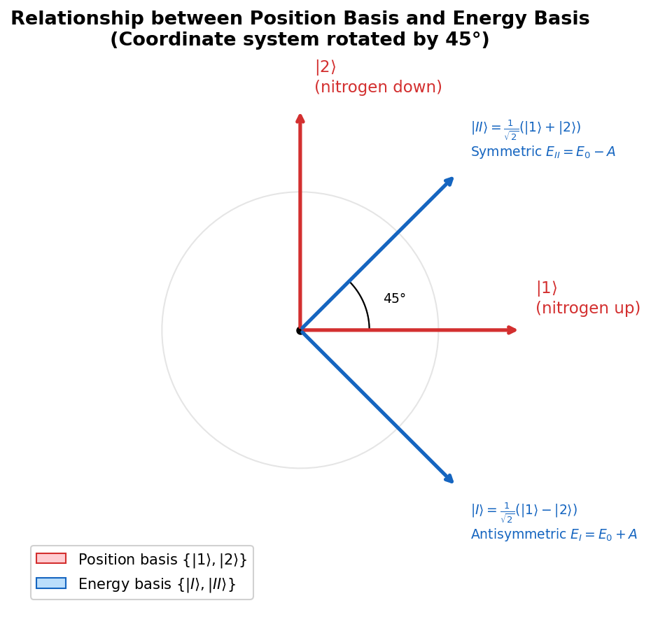
Fig. 6.2: Relationship between position basis and energy basis. The "position basis" \(\{|1\rangle, |2\rangle\}\) and the "energy basis" \(\{|I\rangle, |II\rangle\}\) are related by a 45° rotation. \(|II\rangle\) (symmetric) is an equal sum of \(|1\rangle\) and \(|2\rangle\); \(|I\rangle\) (antisymmetric) is their difference.
🟡 Lina: Let me organize the results so far in a figure. If we plot the potential energy of the ammonia molecule as a function of the nitrogen position, we get two valleys (wells) corresponding to the two stable positions "above" and "below," separated by a central barrier—this is called a double-well potential (Fig. 6.3 "Double-well potential and energy splitting").
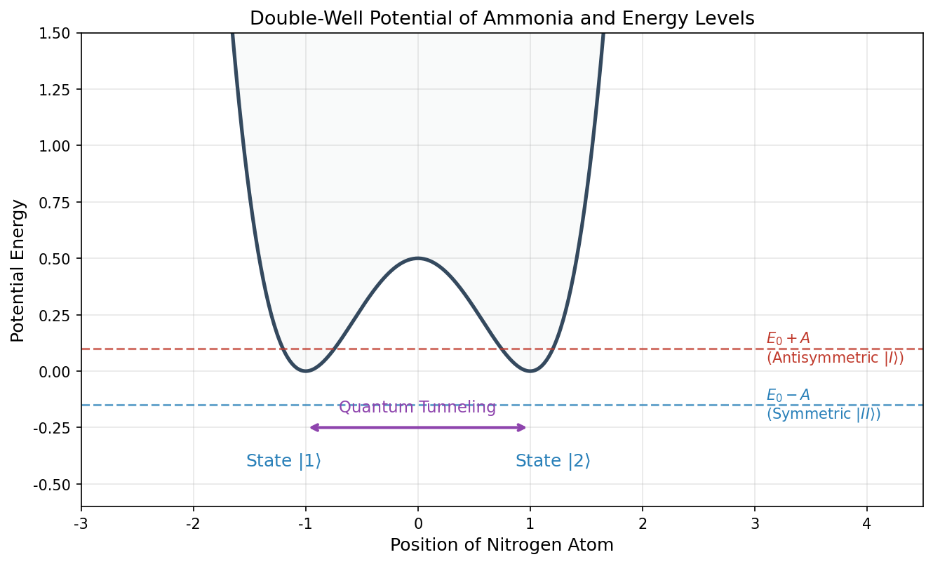
Fig. 6.3: Double-well potential and energy splitting. The double-well potential of the ammonia molecule. There are two wells for state \(|1\rangle\) (nitrogen above) and state \(|2\rangle\) (nitrogen below), with quantum tunneling between them through the barrier. The symmetric state \(|II\rangle\) has energy \(E_0 - A\) (the lower one), and the antisymmetric state \(|I\rangle\) has energy \(E_0 + A\) (the higher one).
✅ Comprehension Check: The tunnel splitting \(2A\) of the ammonia molecule corresponds to a microwave frequency of about 24,000 MHz. If there were no tunneling (\(A = 0\)), what would happen to the energy levels?
Answer
If \(A = 0\), then \(E_I = E_{II} = E_0\), and the two energy levels completely overlap (become degenerate). If nitrogen cannot penetrate the plane, the "above" and "below" configurations are independent and indistinguishable, so no energy difference arises.
📝 Exercises:
- Verify the derivation of the eigenvector corresponding to eigenvalue \(E_I = E_0 + A\), starting from equation (6.9b). → Problem B-4. Verification of Orthogonality of Eigenvectors
6.5 Time Evolution of Stationary States
🟡 Lina: Now that we know the eigenvalues and eigenvectors, we can write down the time evolution of stationary states. A system that is in eigenstate \(|I\rangle\) at initial time \(t = 0\) is at time \(t\):
Similarly for eigenstate \(|II\rangle\):
🔵 Kai: \(e^{-iEt/\hbar}\) always has absolute value 1, right? So \(|C_1|^2\) and \(|C_2|^2\) don't change with time.
🟡 Lina: Exactly. In stationary states, the probabilities of being found in \(|1\rangle\) or \(|2\rangle\) don't depend on time. That's why they're called "stationary."
✅ Comprehension Check: In stationary states, the amplitudes have time dependence \(e^{-iEt/\hbar}\). Why are they called "stationary"?
Answer
\(e^{-iEt/\hbar}\) is a phase factor with absolute value always equal to 1, so the probabilities \(|C_1|^2\) and \(|C_2|^2\) don't depend on time. Since the observable physical quantities (probabilities) don't change, they're called "stationary." What's changing is only the phase of the amplitudes.
⚪ Mei: For example, when in state \(|II\rangle\), the probability of being found in \(|1\rangle\) is \(|1/\sqrt{2}|^2 = 1/2\). The probability of being found in \(|2\rangle\) is also \(1/2\). The probabilities of nitrogen being above or below are always fifty-fifty, and this doesn't change with time.
🟡 Lina: However, the phase of the amplitudes keeps rotating. Since \(e^{-iE_I t/\hbar}\) and \(e^{-iE_{II} t/\hbar}\) rotate at different angular frequencies, if we create a superposition that is not a stationary state—something interesting happens.
6.6 Quantum Oscillations — Time Evolution of Amplitudes Depending on Initial Conditions
🟡 Lina: Here's the highlight of this chapter. Consider the initial condition where at \(t = 0\) the nitrogen is "above"—that is, \(|\psi(0)\rangle = |1\rangle\).
🔵 Kai: \(|1\rangle\) isn't an eigenstate, right? We need to write it as a superposition of \(|I\rangle\) and \(|II\rangle\).
🟡 Lina: Right. Let's add equations (6.15a) and (6.15b) to find \(|1\rangle\):
Therefore:
Similarly, computing \(|II\rangle - |I\rangle\):
Therefore:
🟡 Lina: This is a change of basis. \(\{|1\rangle, |2\rangle\}\) and \(\{|I\rangle, |II\rangle\}\) are both bases for the two-state system, but the latter consists of Hamiltonian eigenstates, so we call it the energy basis.
⚪ Mei: The same state viewed in a position-like basis versus an energy basis—we're just switching perspectives.
🟡 Lina: Right. Now, rewrite \(|\psi(0)\rangle = |1\rangle\) using equation (6.17a), and attach the time evolution phase factor to each eigenstate. Why is this allowed? Because equation (6.2) is linear. For linear equations, "a superposition of solutions is also a solution"—so if we find the time evolution of eigenstate \(|I\rangle\) and of \(|II\rangle\) separately and add them, we get the time evolution of the whole thing:
Converting \(|I\rangle\) and \(|II\rangle\) back to the original basis:
Collecting the coefficient of \(|1\rangle\): the contribution from \(|I\rangle\) is \(\frac{1}{\sqrt{2}} \cdot \frac{1}{\sqrt{2}} = \frac{1}{2}\), and from \(|II\rangle\) is also \(\frac{1}{\sqrt{2}} \cdot \frac{1}{\sqrt{2}} = \frac{1}{2}\):
Similarly, let's find the coefficient of \(|2\rangle\). Using the same method as for \(C_1\), we gather the coefficient of \(|2\rangle\) from each eigenstate. Since \(|I\rangle = \frac{1}{\sqrt{2}}(|1\rangle - |2\rangle)\), the coefficient of \(|2\rangle\) in \(|I\rangle\) is \(-1/\sqrt{2}\). In equation (6.18), \(|I\rangle\) is preceded by \(1/\sqrt{2}\), so the contribution from \(|I\rangle\) to \(|2\rangle\) is \(\frac{1}{\sqrt{2}} \times (-\frac{1}{\sqrt{2}}) = -\frac{1}{2}\). Similarly, in \(|II\rangle = \frac{1}{\sqrt{2}}(|1\rangle + |2\rangle)\), the coefficient of \(|2\rangle\) is \(+1/\sqrt{2}\), and in equation (6.18), \(|II\rangle\) is also preceded by \(1/\sqrt{2}\), so the contribution from \(|II\rangle\) is \(\frac{1}{\sqrt{2}} \times \frac{1}{\sqrt{2}} = +\frac{1}{2}\). Therefore (writing the \(|I\rangle\) contribution first, then the \(|II\rangle\) contribution):
(The last equality just swaps the order of the two terms using \(-a + b = b - a\). The reason for this rewriting is that when we soon substitute \(E_I = E_0 + A\), \(E_{II} = E_0 - A\), we get \(e^{-iE_{II} t/\hbar} - e^{-iE_I t/\hbar} = e^{-i(E_0-A)t/\hbar} - e^{-i(E_0+A)t/\hbar}\), and factoring out the common factor \(e^{-iE_0 t/\hbar}\) gives the form \(e^{+iAt/\hbar} - e^{-iAt/\hbar}\)—which by Euler's formula converts to \(\sin\).)
🔵 Kai: A sum and difference of two complex exponentials... Is this like "beats"?
🟡 Lina: Exactly! Let's factor out the common part. Substituting \(E_I = E_0 + A\), \(E_{II} = E_0 - A\) into equation (6.19a):
The expression in parentheses is \(e^{-iAt/\hbar} + e^{+iAt/\hbar}\). Similarly, organizing \(C_2\):
⚪ Mei: \(C_1\) has a "sum" form and \(C_2\) has a "difference" form—it looks like trigonometric functions will emerge.
🟡 Lina: Here we use Euler's formula. From \(e^{i\theta} = \cos\theta + i\sin\theta\) introduced in Ch. 4, two useful formulas follow:
For \(C_1\), the parentheses contain \(e^{-iAt/\hbar} + e^{+iAt/\hbar} = 2\cos(At/\hbar)\), so multiplying by \(1/2\) gives \(\cos(At/\hbar)\). For \(C_2\), the parentheses contain \(-e^{-iAt/\hbar} + e^{+iAt/\hbar}\). Swapping the order of terms gives \(e^{+iAt/\hbar} - e^{-iAt/\hbar}\)—which is exactly the second formula above with \(\theta = At/\hbar\). So \(e^{+iAt/\hbar} - e^{-iAt/\hbar} = 2i\sin(At/\hbar)\), and multiplying by \(1/2\) gives \(i\sin(At/\hbar)\).
🔵 Kai: Oh wow, they separate cleanly into \(\cos\) and \(i\sin\)!
🟡 Lina: Exactly. And since \(\cos\) and \(\sin\) are offset by \(\pi/2\), the two amplitudes alternately grow larger and smaller—this is the essence of quantum oscillation. In summary:
🟡 Lina: Now let's calculate the probabilities:
🔵 Kai: Wow! The probabilities oscillate back and forth as \(\cos^2\) and \(\sin^2\)... This means the nitrogen atom periodically moves back and forth between above and below!?
🟡 Lina: Exactly. A nitrogen atom that classically shouldn't be able to cross the barrier probabilistically oscillates back and forth in quantum mechanics—this is the essence of quantum oscillations. Let's check this concretely. At \(t = 0\), \(\cos^2(0) = 1\) so \(P_1 = 1\) and nitrogen is indeed above. As time passes, \(P_1\) decreases.
🔵 Kai: \(\cos^2\) becomes zero when... \(At/\hbar = \pi/2\), so at \(t = \pi\hbar/(2A)\), \(P_1 = 0\). Does that mean there's a moment when the nitrogen completely moves to "below"!? Even though it shouldn't be able to cross the barrier!
⚪ Mei: Yes. At that time \(P_2 = \sin^2(\pi/2) = 1\), so it's below with 100% probability. And then it comes back—periodic oscillation.
🟡 Lina: This is called quantum oscillation, or Rabi oscillation. Let's find the angular frequency. Rewriting \(P_1(t) = \cos^2(At/\hbar)\) using the half-angle formula \(\cos^2\theta = \frac{1}{2}(1 + \cos 2\theta)\) gives \(P_1(t) = \frac{1}{2}(1 + \cos(2At/\hbar))\). Looking at this expression, the probability oscillates around a constant value of \(1/2\) with \(\cos(2At/\hbar)\). Since the argument of the \(\cos\) is \(2At/\hbar\), the angular frequency of the probability oscillation is:
The period of oscillation is:
During one period \(T\), the nitrogen atom makes one complete round trip "above → below → above." The graph of this oscillation is shown in Fig. 6.4 "Time dependence of probability due to Rabi oscillation".
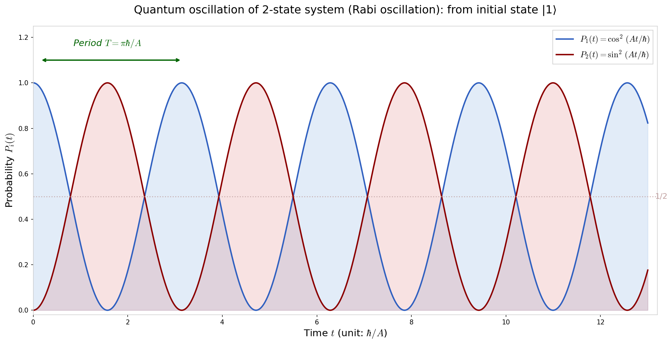
Fig. 6.4: Time dependence of probability due to Rabi oscillation. Rabi oscillation from initial state \(|\psi(0)\rangle = |1\rangle\). \(P_1(t) = \cos^2(At/\hbar)\) (blue) and \(P_2(t) = \sin^2(At/\hbar)\) (red). The probability oscillates completely back and forth, with \(P_1 + P_2 = 1\) holding at all times.
⚪ Mei: Since the probabilities oscillate as \(\cos^2\) and \(\sin^2\), \(P_1 + P_2 = \cos^2 + \sin^2 = 1\) always holds. Probability conservation is confirmed.
🔵 Kai: Wait a moment. The nitrogen atom "slips through" the hydrogen plane, but classically it shouldn't have enough energy, right? Yet the probability grows as \(\sin^2\)... But does \(A\) become smaller when the barrier gets higher? That is, in the limit of infinitely high barrier, tunneling disappears and the oscillation stops?
🟡 Lina: Good question. Exactly right. The higher and thicker the barrier, the more \(A\) decreases exponentially. Classically, the nitrogen atom is blocked by the potential barrier and cannot reach the other side. But in quantum mechanics, as long as the tunneling amplitude \(A\) is not zero, oscillation occurs. If \(A\) is small the oscillation is slow, but for a finite barrier it never truly becomes zero.
🔵 Kai: "Decreases exponentially" means that even a slightly thicker barrier causes \(A\) to plummet... So at everyday scales, barriers are astronomically thick compared to atomic scales, making the probability of passing through effectively zero?
🟡 Lina: Exactly. For macroscopic objects, barriers are enormously thick compared to atomic scales, so \(A\) becomes astronomically small. But conversely, as long as \(A\) is finite—that is, as long as the barrier has finite height and width—quantum oscillation never completely vanishes. The only limit where it "completely stops" is when the barrier is infinite. This is the essential difference from classical mechanics.
⚪ Mei: In other words, what's an "impenetrable wall" in classical mechanics becomes merely a "hard-to-penetrate wall" in quantum mechanics—it's a matter of degree, and in principle it never reaches zero.
✅ Comprehension Check: How is the angular frequency \(\omega_0\) of Rabi oscillation expressed? Also, does the oscillation become faster or slower when the tunneling amplitude \(A\) is larger?
Answer
\(\omega_0 = 2A/\hbar\). The larger \(A\) is, the larger the angular frequency, so the oscillation is faster. The stronger the tunneling effect (the easier it is to penetrate the barrier), the more frequently nitrogen oscillates between above and below.
✅ Comprehension Check: If the initial state were \(|\psi(0)\rangle = |2\rangle\) (nitrogen "below"), what would \(P_1(t)\) and \(P_2(t)\) be?
Answer
From equation (6.17b), \(|2\rangle = \frac{1}{\sqrt{2}}(-|I\rangle + |II\rangle)\). Performing a similar calculation gives \(P_1(t) = \sin^2(At/\hbar)\), \(P_2(t) = \cos^2(At/\hbar)\). In other words, only the initial condition is swapped, and the oscillation pattern is the same (\(\cos\) and \(\sin\) are exchanged).
📝 Exercises:
- When the initial state is \(|\psi(0)\rangle = |II\rangle\) (the low-energy eigenstate), calculate \(P_1(t)\) and \(P_2(t)\) and confirm that they are time-independent. → Problem B-5. Calculating the Time Dependence of Probability
6.7 Why the Hamiltonian Is Central — A Review So Far
🔵 Kai: Looking back at all this, the Hamiltonian matrix is really powerful. Just writing down one matrix gives you energy levels, stationary states, and time evolution—everything.
🟡 Lina: Right. "Solving a problem" in quantum mechanics ultimately means writing down the Hamiltonian and finding its eigenvalues and eigenvectors. Here's the procedure summarized:
- Choose a basis: Set up physically natural basis states \(\{|1\rangle, |2\rangle, \ldots\}\)
- Determine the Hamiltonian matrix: Use symmetry and physical reasoning to determine \(H_{ij}\)
- Solve the eigenvalue problem: \(H|E_n\rangle = E_n|E_n\rangle\) — obtain energy levels \(E_n\) and eigenstates \(|E_n\rangle\)
- Expand the initial condition in eigenstates: \(|\psi(0)\rangle = \sum_n c_n |E_n\rangle\)
- Write the time evolution: \(|\psi(t)\rangle = \sum_n c_n\,e^{-iE_n t/\hbar}|E_n\rangle\)
Table 6.2: Five steps for solving a quantum mechanics problem
| Step | Operation | Concrete example for ammonia |
|---|---|---|
| 1. Choose a basis | List physically natural states | \(\|1\rangle\) (N above), \(\|2\rangle\) (N below) |
| 2. Determine the Hamiltonian | Use symmetry and physical reasoning | \(H = \begin{pmatrix} E_0 & -A \\\\ -A & E_0 \end{pmatrix}\) |
| 3. Solve the eigenvalue problem | \(\det(H - E\mathbb{1}) = 0\) | \(E_I = E_0 + A\), \(E_{II} = E_0 - A\) |
| 4. Expand the initial condition | \(c_n = \langle E_n\|\psi(0)\rangle\) | \(\|1\rangle = \frac{1}{\sqrt{2}}(\|I\rangle + \|II\rangle)\) |
| 5. Write the time evolution | Attach \(e^{-iE_n t/\hbar}\) to each eigenstate | \(P_1(t) = \cos^2(At/\hbar)\) (Rabi oscillation) |
⚪ Mei: This recipe applies not just to two-state systems but has the same structure for systems with many more states.
🟡 Lina: Exactly. From Ch. 7 onward, we'll introduce the wave function and the Schrödinger equation, but the basic logical structure is the same as what we've seen here. The eigenvalues of the Hamiltonian are energies, eigenstates are stationary states, and general states evolve in time as superpositions of eigenstates—this skeleton runs through all of quantum mechanics.
🔵 Kai: Practicing with two-state systems seems like it'll make things easier later... But if there are 3 or more states, won't finding eigenvalues become really hard? Cubic equations might come up.
🟡 Lina: Good concern. Indeed, for an \(N\)-state system you need to solve an \(N\)th-degree equation. But in many cases, you can use symmetry to decompose the problem into smaller blocks. We'll see that in later chapters.
🔵 Kai: Symmetry comes up again. With ammonia, symmetry determined \(H_{11} = H_{22}\)... Conversely, for systems without symmetry, determining the Hamiltonian becomes much harder?
🟡 Lina: Exactly. The less symmetry a system has, the more experimental data or other theoretical considerations you need to determine the Hamiltonian components. But conversely, finding symmetry is your greatest weapon for solving problems—a lesson that applies not just to quantum mechanics but to all of physics.
🔵 Kai: "Finding symmetry is your weapon"... Indeed, with ammonia a single up-down symmetry determined half the matrix.
✅ Comprehension Check: Describe the basic procedure for "solving a problem" in quantum mechanics in five steps.
Answer
(1) Choose a basis, (2) determine the Hamiltonian matrix, (3) solve the eigenvalue problem to get energy levels and eigenstates, (4) expand the initial condition in eigenstates, (5) attach the phase factor \(e^{-iE_n t/\hbar}\) to each eigenstate to write the time evolution.
6.8 The Ammonia Molecule in an Electric Field — When Symmetry Is Broken
🟡 Lina: Let's now take one more step and consider what happens when an external electric field is applied to the ammonia molecule.
🔵 Kai: What changes when you apply an electric field?
🟡 Lina: The ammonia molecule possesses an electric dipole moment \(\mu\). An electric dipole moment is a quantity representing the magnitude and direction of the offset when the centers of positive and negative charge within a molecule are displaced from each other. Quantitatively, when a positive charge \(q\) and negative charge \(-q\) are separated by distance \(d\), the magnitude of the dipole moment is defined as \(\mu = qd\). Its dimensions are \([\text{charge}] \times [\text{length}]\), and the SI unit is C·m (coulomb-meter).
🔵 Kai: Positive and negative are offset... What does that mean concretely?
🟡 Lina: The nitrogen atom attracts electrons more strongly than the hydrogen atoms. So the nitrogen side becomes slightly negative (\(-\)) and the hydrogen side slightly positive (\(+\)). The direction of the dipole moment is defined as pointing from negative charge to positive charge. Remember it as "an arrow pointing from \(-\) to \(+\)." Looking at Fig. 6.1 "Structure of the ammonia molecule" again—in the configuration with nitrogen (\(-\)) above and hydrogen (\(+\)) below, the arrow points from above (\(-\)) to below (\(+\)), so the dipole is "downward." In the configuration with nitrogen "below," it's the opposite: the dipole is "upward."
Now let me discuss the energy when a dipole is placed in an electric field. The positive charge is pulled in the direction of the field, and the negative charge is pulled in the opposite direction. So when the dipole arrow is aligned with the field—that is, when the positive charge side is in the field direction—is the most stable and lowest energy. When it's opposite, it's most unstable and highest energy. We say the "dipole is aligned with the field."
🔵 Kai: Let me organize this. When nitrogen is "above," the negative charge (nitrogen side) is on top and positive charge (hydrogen side) is on the bottom... The arrow points from the \(-\) above to the \(+\) below. So the dipole is "downward." If nitrogen is "below," then negative charge is at the bottom and positive at the top, so the arrow goes from bottom to top—"upward."
⚪ Mei: "The dipole arrow points from \(-\) to \(+\)"—as long as you remember this, once the nitrogen position is determined, the arrow direction is determined too.
🟡 Lina: Exactly. You confirmed that carefully. The key point is that the "arrow direction" and "nitrogen position" are always opposite—nitrogen above means arrow down, nitrogen below means arrow up. Keep this correspondence in mind.
⚪ Mei: When the nitrogen position flips, the dipole moment direction also flips.
🟡 Lina: Right. Let's apply an external electric field \(\mathcal{E}\) pointing "upward." When a dipole is placed in an electric field, the positive charge side is pulled in the field direction and the negative charge side is pulled opposite. When the dipole is aligned with the field it's "stable" and energy is low; when opposite it's "unstable" and energy is high. Quantitatively, the interaction energy between dipole moment and electric field is \(U = -\mu\mathcal{E}\cos\theta\) (where \(\theta\) is the angle between the dipole and the field). To briefly explain the origin of this formula: the positive charge \(+q\) feels a force \(F = qE\) in the field direction, and the negative charge \(-q\) feels an equal force in the opposite direction. When the dipole makes angle \(\theta\) with the field, the "effective length" in the field direction is \(d\cos\theta\), so the work (energy) is \(-qd\mathcal{E}\cos\theta = -\mu\mathcal{E}\cos\theta\). When aligned (\(\theta = 0°\)), energy is lowest: \(U = -\mu\mathcal{E}\); when anti-aligned (\(\theta = 180°\)), energy is highest: \(U = +\mu\mathcal{E}\).
🔵 Kai: Alignment lowers energy, anti-alignment raises it... similar to how a magnet tends to align with a magnetic field.
🟡 Lina: Good analogy. Let's verify concretely. In state \(|1\rangle\) with nitrogen "above," as we just confirmed, the dipole is downward. The field is upward, so the dipole and field are anti-aligned (\(\theta = 180°\)) and \(U = +\mu\mathcal{E}\) (energy is high). In state \(|2\rangle\) with nitrogen "below," the dipole is upward, same direction as the field (\(\theta = 0°\)), so \(U = -\mu\mathcal{E}\) (energy is low).
🔵 Kai: So \(H_{11} \neq H_{22}\)! The symmetry is broken!
🟡 Lina: Exactly. The Hamiltonian in the electric field is:
Here, we're assuming the tunneling amplitude \(-A\) is hardly affected by the electric field.
🔵 Kai: I'd like to see in a figure how the energy levels move as we change the field.
🟡 Lina: Good suggestion. Look at Fig. 6.5 "Energy levels in an electric field". If \(A = 0\) (no tunneling), the two energy levels change linearly and cross at \(\mu\mathcal{E} = 0\) (dashed lines). But when \(A \neq 0\), where they would have crossed, the levels "repel each other"—this is called an avoided crossing. I'll calculate the eigenvalues shortly, but giving the result ahead of time: the level spacing becomes \(2\sqrt{A^2 + \mu^2\mathcal{E}^2}\). As long as \(A \neq 0\), this never becomes zero—the two levels never cross. The closest approach (at \(\mathcal{E} = 0\)) has spacing \(2A\).
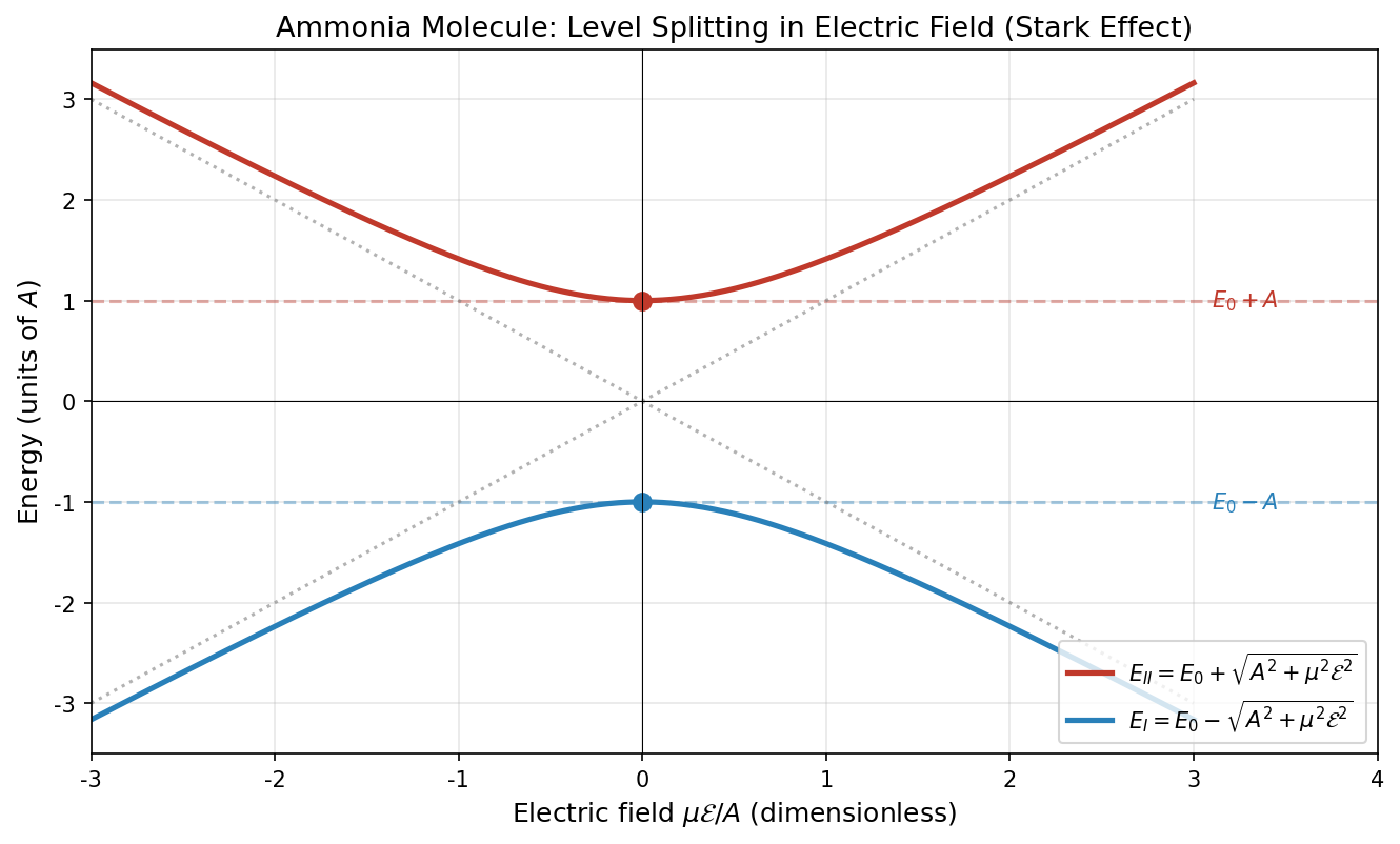
Fig. 6.5: Energy levels in an electric field. Horizontal axis is \(\mu\mathcal{E}/A\), vertical axis is energy. Dashed lines show the case \(A = 0\) (no tunneling), where two straight lines cross. Solid lines show \(A \neq 0\), where the crossing is avoided (avoided crossing), with minimum spacing \(2A\).
Eigenvalues in the Electric Field
🟡 Lina: Let's find the eigenvalues. The eigenvalues of a general two-state Hamiltonian
are:
🔵 Kai: Where does this come from?
🟡 Lina: The same procedure as the previous section. Writing \(\det(H - E\mathbb{1}) = 0\) for general components: \((H_{11} - E)(H_{22} - E) - H_{12}H_{21} = 0\)—just using the determinant definition \(ad - bc\) with \(a = H_{11} - E\), \(b = H_{12}\), \(c = H_{21}\), \(d = H_{22} - E\). Expanding this, and using Hermiticity to write \(H_{12}H_{21} = H_{12}H_{12}^* = |H_{12}|^2\):
This is a quadratic equation in \(E\), so using the quadratic formula from high school: \(E = \frac{(H_{11}+H_{22}) \pm \sqrt{(H_{11}+H_{22})^2 - 4(H_{11}H_{22} - |H_{12}|^2)}}{2}\). Simplifying the discriminant: \((H_{11}+H_{22})^2 - 4H_{11}H_{22} + 4|H_{12}|^2 = (H_{11}-H_{22})^2 + 4|H_{12}|^2\), giving equation (6.25). This is a general formula applicable to any two-state Hamiltonian, not just ammonia.
⚪ Mei: So as long as you know \(H_{11}\), \(H_{22}\), and \(H_{12}\), you can immediately find the eigenvalues.
🟡 Lina: For the ammonia molecule, substituting \(H_{11} + H_{22} = 2E_0\), \(H_{11} - H_{22} = 2\mu\mathcal{E}\), \(|H_{12}|^2 = A^2\):
🔵 Kai: When \(\mathcal{E} = 0\), \(\sqrt{A^2} = A\), so \(E_I = E_0 + A\), \(E_{II} = E_0 - A\)—back to what we had before.
🟡 Lina: Right. As the field gets stronger, the level spacing \(E_I - E_{II} = 2\sqrt{A^2 + \mu^2\mathcal{E}^2}\) increases.
Limiting Behavior
🟡 Lina: Let's look at two limits.
Weak field (\(\mu\mathcal{E} \ll A\)):
Here we used the approximation \(\sqrt{1+x} \approx 1 + x/2\) (when \(x \ll 1\)). This is the first-order Taylor expansion of \((1+x)^{1/2}\)—"when \(x\) is sufficiently small, ignore terms of \(x^2\) and higher and keep only the first-order term." Testing with \(x = 0.01\): \(\sqrt{1.01} = 1.00499\ldots \approx 1 + 0.005 = 1.005\)—a good match.
Therefore:
⚪ Mei: The energy change is proportional to \(\mathcal{E}^2\). Interesting that it's the square, not the first power.
🟡 Lina: Right. When the energy change is proportional to \(\mathcal{E}^2\), the proportionality constant is called the polarizability. Here \(\mu^2/(2A)\) plays that role. The smaller \(A\) is, the larger the polarizability—meaning greater sensitivity to the field. Intuitively, a small \(A\) means the two levels are close together. The closer the levels, the more easily an external perturbation (electric field) mixes the states, causing larger energy shifts. The ammonia molecule has a very small \(A\) (on the microwave energy scale), so its polarizability is anomalously large.
🔵 Kai: Close levels mean field sensitivity... It's like something in an unstable balance that moves a lot with just a small push.
🟡 Lina: Strong field (\(\mu\mathcal{E} \gg A\)):
🔵 Kai: Does this mean \(A\) no longer matters?
🟡 Lina: Right. When the field is very strong, the energy difference \(2\mu\mathcal{E}\) between "above" and "below" overwhelms the tunneling amplitude \(A\). The nitrogen atom gets "pinned" to the lower-energy side, and the effect of tunneling to the other side becomes barely visible.
🔵 Kai: A strong field "kills" the tunneling effect. Intuitively that makes sense—the energy slope is too steep for tunneling to matter.
🟡 Lina: Let me summarize the two limits in a table.
Table 6.3: Comparison of behavior for weak and strong fields
| Weak field (\(\mu\mathcal{E} \ll A\)) | Strong field (\(\mu\mathcal{E} \gg A\)) | |
|---|---|---|
| Field dependence of energy | Proportional to \(\mathcal{E}^2\) (quadratic) | Proportional to \(\mathcal{E}\) (linear) |
| Level spacing | \(\approx 2A\) (nearly constant) | \(\approx 2\mu\mathcal{E}\) (proportional to field) |
| Character of eigenstates | Symmetric/antisymmetric (\(\|1\rangle \pm \|2\rangle\)) | Nearly \(\|1\rangle\) and \(\|2\rangle\) (localized) |
| Effect of tunneling | Dominant (quantum oscillation occurs) | Suppressed (nitrogen pinned to one side) |
| Physical picture | Nitrogen oscillates between above and below | Nitrogen remains on the lower-energy side |
✅ Comprehension Check: In the weak-field limit (\(\mu\mathcal{E} \ll A\)), the field dependence of the energy levels is proportional to what power of \(\mathcal{E}\)? What is the proportionality constant called?
Answer
In the weak-field limit, the energy change is proportional to \(\mathcal{E}^2\) (a second-order effect). The proportionality constant \(\mu^2/(2A)\) is called the polarizability. The smaller \(A\) is, the larger the polarizability, making the system more sensitive to the field.
✅ Comprehension Check: When the electric field \(\mathcal{E}\) is gradually increased, how does the spacing between energy levels \(E_I\) and \(E_{II}\) change?
Answer
\(E_I - E_{II} = 2\sqrt{A^2 + \mu^2\mathcal{E}^2}\). At \(\mathcal{E} = 0\) it's \(2A\); it monotonically increases with \(\mathcal{E}\); and for \(\mathcal{E} \gg A/\mu\) it approaches \(2\mu\mathcal{E}\). The level spacing only widens with the field and never narrows.
📝 Exercises:
- Derive equation (6.25) from the quadratic formula. → Problem M-1. Derivation of Hermiticity from Probability Conservation
6.9 The Principle of the Ammonia Maser — Transitions Driven by an Oscillating Electric Field
🟡 Lina: Finally, let's touch on the operating principle of the ammonia maser. MASER stands for Microwave Amplification by Stimulated Emission of Radiation.
🔵 Kai: In Ch. 1, there was talk about Einstein's stimulated emission (1917). Is this related?
🟡 Lina: Exactly. The maser realizes stimulated emission, predicted by Einstein, using the two-level system of ammonia molecules. In 1954, Townes and colleagues demonstrated the first working device, which became the prototype for the later LASER.
Molecular Separation
🟡 Lina: Operating the maser requires preparation. First, we create a beam of ammonia molecules and separate molecules in state \(|I\rangle\) (high energy) from those in state \(|II\rangle\) (low energy).
🔵 Kai: How do you separate them?
🟡 Lina: Using an inhomogeneous electric field. Look at equation (6.27). In the weak-field approximation:
- The energy of state \(|I\rangle\) increases with \(\mathcal{E}^2\)
- The energy of state \(|II\rangle\) decreases with \(\mathcal{E}^2\)
In high school physics you learned that "objects experience a force toward regions of lower potential energy." That is, the force is \(F = -dU/dx\)—in the direction where energy increases, a restoring force pushes back. In an inhomogeneous field, the field strength \(\mathcal{E}\) varies with position, so the molecule's energy also varies with position. Molecules in state \(|I\rangle\) have energy that increases with \(\mathcal{E}^2\), so energy is higher where the field is stronger—therefore they experience a force toward the weaker field region. Conversely, molecules in state \(|II\rangle\) have energy that decreases with \(\mathcal{E}^2\), so energy is lower where the field is stronger—they experience a force toward the stronger field region. This splits the beam into two.
🔵 Kai: Oh, isn't this similar to the Stern-Gerlach experiment in Ch. 5? There, an inhomogeneous magnetic field separated spins.
🟡 Lina: Good connection. It's exactly the same idea. Stern-Gerlach used an inhomogeneous magnetic field and the spin's magnetic moment, whereas here we use an inhomogeneous electric field and the electric dipole moment—the physical mechanism is the same: "energy depends on field strength → force in an inhomogeneous field → separation by state." After separation, only molecules in state \(|I\rangle\) (high energy) are fed into a cavity resonator.
Time-Dependent Electric Field and Transitions
🟡 Lina: Inside the cavity resonator, there's an electric field oscillating at frequency \(\omega\): \(\mathcal{E}(t) = \mathcal{E}_0 \cos\omega t\). Since the Hamiltonian is now time-dependent, we can't solve it just by "finding eigenvalues."
🔵 Kai: A time-dependent Hamiltonian... that sounds hard.
🟡 Lina: In general it is, but when the field is weak (\(\mu\mathcal{E}_0 \ll A\)), it can be solved approximately. The trick is to separate the "fast oscillation without the field" from the "slow change due to the field."
🔵 Kai: What does "separate" mean concretely?
🟡 Lina: Without the field, the eigenstate amplitudes just rotate their phase rapidly: \(C_I(t) = (\text{constant}) \times e^{-iE_I t/\hbar}\). The idea is to remove this "known fast rotation" in advance and track only the "new change caused by the field." Specifically:
Without the field, \(\gamma_I\) and \(\gamma_{II}\) are constants that don't change. With the field, \(\gamma_I\) and \(\gamma_{II}\) change slowly. This way, the equations of motion for \(\gamma\) have the "fast oscillation" removed, leaving only the field's effect—making things much clearer.
⚪ Mei: I see—"subtract the known rotation and look at what remains"—like removing background.
🟡 Lina: Let me show the path to rewriting the equations of motion for \(\gamma_I\) and \(\gamma_{II}\). It's a bit long, but follow step by step.
First, differentiating \(C_I(t) = \gamma_I(t)\,e^{-iE_I t/\hbar}\) from equation (6.29), using the product rule:
Putting this into the left side of equation (6.2), \(i\hbar\,dC_I/dt\):
Meanwhile, the right side uses the Hamiltonian in the field \(H = H_0 + V(t)\). Here \(H_0\) is the field-free Hamiltonian (with eigenvalues \(E_I\), \(E_{II}\)), and \(V(t)\) is the perturbation due to the field. Written in the energy basis \(\{|I\rangle, |II\rangle\}\), the \(H_0\) contribution is diagonal and produces \(E_I\,\gamma_I\,e^{-iE_I t/\hbar}\) (the part corresponding to stationary rotation). The same term appears on the left side, so it cancels from both sides, leaving only the off-diagonal terms from \(V(t)\).
🔵 Kai: Wait. "\(V(t)\) is off-diagonal"—but in the position basis \(\{|1\rangle, |2\rangle\}\), \(V\) was diagonal, right? Does it become off-diagonal in the energy basis?
🟡 Lina: Good question. That's exactly the point. In the position basis, \(\langle 1|V|1\rangle = +\mu\mathcal{E}_0\cos\omega t\), \(\langle 2|V|2\rangle = -\mu\mathcal{E}_0\cos\omega t\), and \(\langle 1|V|2\rangle = \langle 2|V|1\rangle = 0\)—diagonal. But computing the off-diagonal element \(\langle I|V|II\rangle\) in the energy basis, substituting \(|I\rangle = \frac{1}{\sqrt{2}}(|1\rangle - |2\rangle)\), \(|II\rangle = \frac{1}{\sqrt{2}}(|1\rangle + |2\rangle)\):
⚪ Mei: I see. A perturbation that was diagonal in the position basis generates off-diagonal elements in the energy basis—it becomes a term coupling \(|I\rangle\) and \(|II\rangle\). It's interesting how "diagonal vs. off-diagonal" swaps depending on the choice of basis.
🟡 Lina: Exactly. Changing bases is like rotating coordinate axes—the matrix looks different but the physical content is the same. Check the detailed full derivation in the exercises.
Now, organizing: the \(\gamma_{II}\) appearing on the right side originally had \(e^{-iE_{II} t/\hbar}\) attached via \(C_{II} = \gamma_{II}\,e^{-iE_{II} t/\hbar}\), which combines with \(e^{+iE_I t/\hbar}\) from the left side to give \(e^{-i(E_{II} - E_I)t/\hbar} = e^{i\omega_0 t}\) (where \(\omega_0 = (E_I - E_{II})/\hbar = 2A/\hbar\)). Furthermore, rewriting \(\cos\omega t = \frac{1}{2}(e^{i\omega t} + e^{-i\omega t})\), two types of factors multiply \(\gamma_{II}\): \(e^{i(\omega_0 + \omega)t}\) and \(e^{i(\omega_0 - \omega)t}\). That is:
🔵 Kai: So two types of oscillating factors appear: \(\omega_0 + \omega\) and \(\omega_0 - \omega\)...
🟡 Lina: The former (oscillating at \(\omega_0 + \omega\)) rapidly alternates between positive and negative at a very high frequency. Meanwhile, how fast does \(\gamma\) change? The entire right side acts as the "driving force" changing \(\gamma\), and its magnitude is determined by the coefficient \(\mu\mathcal{E}_0/(2\hbar)\). Recall from high school that for \(dy/dt = ky\), the solution \(y = y_0 e^{kt}\)—the time for \(y\) to change significantly is on the order of \(1/k\). Our coupled equations have the form \(d\gamma_I/dt \sim (\mu\mathcal{E}_0/\hbar)\,\gamma_{II}\), so the coefficient \(\mu\mathcal{E}_0/\hbar\) on the right side determines the "speed of change." Strictly speaking, it's a coupled system so it's not a simple exponential, but the time scale of change is of order the inverse of the coefficient—roughly \(\hbar/(\mu\mathcal{E}_0)\).
🔵 Kai: So \(\gamma\) changes slowly? But why does the "rapidly oscillating term" vanish? Even if it oscillates rapidly, it's not zero...
🟡 Lina: Good question. Think of it this way. During the short time that \(\gamma\) barely changes, the rapidly oscillating term \(e^{i(\omega_0+\omega)t}\) goes through many cycles of positive and negative. The "force" changing \(\gamma\) alternates rapidly between positive and negative, so the pushes in the positive direction and pushes in the negative direction almost perfectly cancel. If you push and pull a swing at super-high speed randomly, the swing barely moves, right? Same idea. Meanwhile, the \(e^{i(\omega_0-\omega)t}\) term, when \(\omega \approx \omega_0\), barely oscillates and keeps "pushing in the same direction," so the effect accumulates.
⚪ Mei: The swing analogy is clear. A force that rapidly alternates in sign is effectively zero; only the slow force has an effect.
🟡 Lina: Right. Remember the condition \(\mu\mathcal{E}_0 \ll A\). The smaller the denominator, the larger the fraction, so \(\mu\mathcal{E}_0 \ll A\) means \(\hbar/(\mu\mathcal{E}_0) \gg \hbar/A\)—that is, the time scale of \(\gamma\)'s change, \(\hbar/(\mu\mathcal{E}_0)\), is much longer than the time scale of rapid oscillation, \(\hbar/A\) (of order \(1/(\omega_0 + \omega)\)). For concrete numbers: for ammonia, \(\omega_0 = 2A/\hbar \sim 2\pi \times 24{,}000\) MHz, so taking \(\omega_0 + \omega \sim 2\omega_0\), one period of rapid oscillation is about \(10^{-11}\) seconds. Meanwhile, with weak field where \(\mu\mathcal{E}_0\) is 1/100 of \(A\), it takes about \(10^{-9}\) seconds for \(\gamma\) to change significantly—100 times slower. So the rapidly oscillating term repeats positive and negative many times while \(\gamma\) barely changes, canceling out to effectively zero—this is called the rotating wave approximation. The name comes from \(e^{i\omega t}\) representing a "rotating wave" in the complex plane. We drop the fast-rotating component and keep only the slowly rotating one—hence "rotating wave approximation." Keeping only the latter, the equation for \(\gamma_I\) approximately becomes:
(Approximate equations under the rotating wave approximation. For the complete derivation, see Problem M-2. Derivation of Rabi Oscillations.) Let me explain why the sign in the exponential of equation (6.30b) is opposite to (6.30a). In the equation for \(\gamma_{II}\), removing \(e^{-iE_{II} t/\hbar}\) involves multiplying by \(e^{+iE_{II} t/\hbar}\), which combines with the \(e^{-iE_I t/\hbar}\) attached to \(\gamma_I\) to give \(e^{-i(E_I - E_{II})t/\hbar} = e^{-i\omega_0 t}\)—exactly the sign reversal from the \(\gamma_I\) equation. The two equations form a pair, with \(\gamma_I\) and \(\gamma_{II}\) coupled to each other.
🔵 Kai: The form of equation (6.30) looks similar to equation (6.2) from the beginning. \(\gamma_I\) and \(\gamma_{II}\) influence each other.
🟡 Lina: The key is the factor \(e^{\pm i(\omega_0 - \omega)t}\). Here \(\omega_0 = (E_I - E_{II})/\hbar = 2A/\hbar\) is the same quantity as the Rabi oscillation angular frequency we found in equation (6.22). Under the resonance condition \(\omega \approx \omega_0\), \(e^{\pm i(\omega_0 - \omega)t} \approx 1\) stays constant, the effect accumulates, and transitions occur most efficiently.
🔵 Kai: Resonance...? Why do transitions occur more easily when the frequencies match?
🟡 Lina: Imagine a swing. When you push in sync with the swing's period, the "push" accumulates each time and the swing goes higher and higher. But if the timing is off, sometimes you push forward, sometimes you hinder, and the effects cancel out.
🔵 Kai: Mathematically, why does this happen?
🟡 Lina: Look at equation (6.30). The factor \(e^{i(\omega_0 - \omega)t}\) on the right side is the key. Going back to the swing analogy, this factor represents "the timing mismatch between pushing and swinging." If \(\omega = \omega_0\), then \(e^{i \cdot 0 \cdot t} = 1\)—you're pushing at the same timing every time, so the effect accumulates in one direction. But if \(\omega \neq \omega_0\), then \(e^{i(\omega_0 - \omega)t}\) rotates around the complex plane, giving positive contributions (forward pushes) at some times and negative contributions (hindrances) at others, canceling over long times. So only when the external field frequency matches \(\omega_0 = 2A/\hbar\) does the transition probability accumulate efficiently. When the resonance condition is met, molecules transition from \(|I\rangle\) to \(|II\rangle\) and emit the energy difference \(E_I - E_{II} = 2A\) as a microwave photon.
🔵 Kai: The energy difference directly becomes the photon energy. By the relation \(E = h\nu\).
🟡 Lina: This is the stimulated emission predicted by Einstein in 1917. The external field (microwaves already in the cavity) prompts the molecule to "emit a photon." The emitted photon has the same frequency and same phase as the external field, so the microwaves are amplified.
⚪ Mei: Same frequency and same phase means coherent (phase-aligned) microwave source.
🟡 Lina: Exactly. To summarize the maser's operation:
- Molecular preparation: Select molecules in high-energy state \(|I\rangle\) using an inhomogeneous electric field
- Introduction to cavity resonator: Send molecules into a cavity containing microwaves at resonance frequency \(\omega_0 = 2A/\hbar\)
- Stimulated emission: Molecules transition \(|I\rangle \to |II\rangle\) and emit microwave photons
- Amplification: Emitted photons strengthen the microwaves in the cavity
🟡 Lina: Fig. 6.6 "Operating principle of the ammonia maser" shows these four steps schematically.
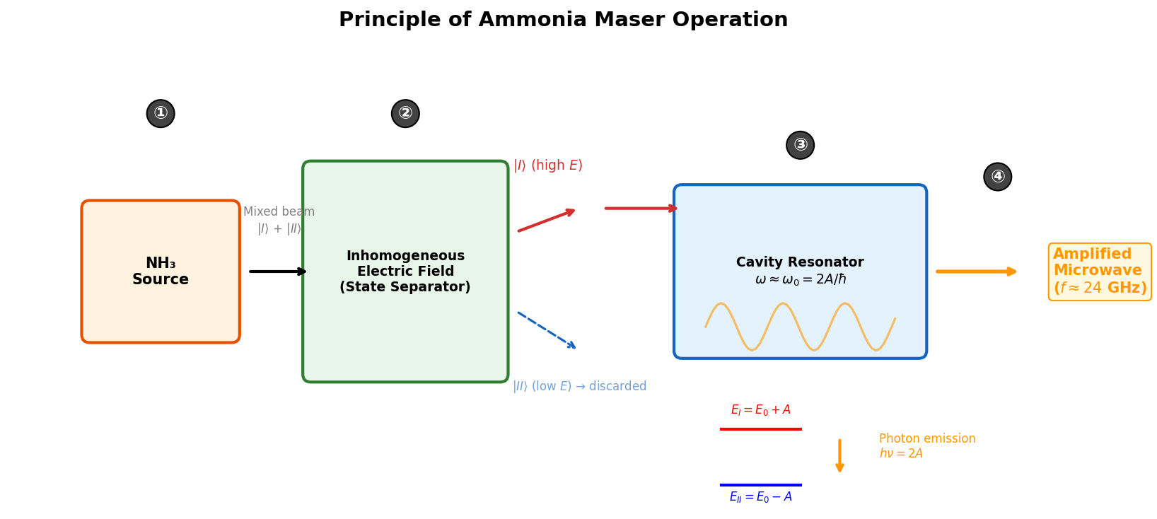
Fig. 6.6: Operating principle of the ammonia maser. ① Mixed beam emitted from NH₃ molecular source → ② High-energy state \(|I\rangle\) selected by inhomogeneous electric field → ③ Introduced into cavity resonator at resonance frequency \(\omega_0 = 2A/\hbar\) to induce stimulated emission → ④ Amplified coherent microwaves (about 24 GHz) are output.
🔵 Kai: Amazing! The theory of a quantum two-state system directly becomes the operating principle of an actual device... But I have one question. Why do you need to select only the high-energy state \(|I\rangle\) molecules? Won't the low-energy \(|II\rangle\) ones work?
🟡 Lina: Good question. Molecules in \(|II\rangle\) would absorb a photon and jump up to \(|I\rangle\)—that is, they would weaken the microwaves. For amplification, there must be more molecules that emit photons. That's why high-energy state molecules must be selected and fed in. This is called population inversion.
🔵 Kai: I understand that you need more emitting molecules. But if you just gather molecules normally, wouldn't the high-energy and low-energy molecules be about fifty-fifty? Even without separation, wouldn't emission and absorption be about equal, netting to zero?
🟡 Lina: Great observation. Actually, in normal conditions (thermal equilibrium), there are more molecules in the low-energy state \(|II\rangle\). At finite temperature, molecules preferentially populate lower-energy states—this is a basic result of statistical mechanics called the Boltzmann distribution. So without intervention, there are more molecules absorbing photons (\(|II\rangle \to |I\rangle\)) than emitting (\(|I\rangle \to |II\rangle\)), and microwaves get weaker. For amplification, you need to artificially make the high-energy state the majority—create a population inversion. This is the key to the maser.
🔵 Kai: I see... In nature the low-energy side is the majority, so you need to deliberately use an inhomogeneous field to select out the high-energy molecules.
🟡 Lina: Exactly. And extending this principle to the optical domain gives us the LASER. When we treat Einstein's A and B coefficients and stimulated emission quantitatively in Ch. 21, we'll return to this topic.
✅ Comprehension Check: Explain why the resonance condition is important in the ammonia maser.
Answer
When the external field frequency \(\omega\) matches the frequency \(\omega_0 = 2A/\hbar\) corresponding to the energy difference between the two levels, the \(|I\rangle \to |II\rangle\) transition occurs most efficiently. When the frequency is detuned, the transition probability drops sharply and microwave amplification doesn't occur.
📝 Exercises:
- Find the wavelength of a photon corresponding to the resonance frequency \(f_0 = \omega_0/(2\pi) = 24{,}000\) MHz of the ammonia molecule. What region of the electromagnetic spectrum does this belong to? → Problem M-3. Energy Levels of an Ammonia Molecule in an Electric Field
6.10 General Formulas for Two-State Systems — Summary
🟡 Lina: Let me summarize the results of this chapter for a general two-state Hamiltonian
that is time-independent. I'll write the energy eigenvalues as \(E_+\), \(E_-\).
🔵 Kai: Wait, before you were writing \(E_I\), \(E_{II}\), but now it's \(E_+\), \(E_-\). Why the change in notation?
🟡 Lina: Good catch. Since we're summarizing as general formulas not limited to ammonia, I changed the notation. \(E_I\), \(E_{II}\) are labels specific to ammonia, while \(E_+\), \(E_-\) are general symbols "usable for any two-state system." The correspondence is simple: \(+\) is the higher one, \(-\) is the lower one:
For ammonia, \(E_+ = E_0 + A\), \(E_- = E_0 - A\). Below, for general two-state systems I'll use \(E_\pm\).
Energy eigenvalues (restatement of equation (6.25), unified to \(E_\pm\) notation):
Time evolution of stationary states:
Time evolution of a general state:
where \(c_{\pm} = \langle E_{\pm}|\psi(0)\rangle\) are determined by the initial conditions.
⚪ Mei: This recipe is a general framework applicable not just to ammonia but to any two-state system.
🟡 Lina: Right. The two-state system is the most basic system in quantum mechanics, yet a surprisingly large number of physical phenomena can be understood within this framework. For example, the behavior of a spin-1/2 particle in a magnetic field is also like this. In Ch. 17, we'll describe spin-1/2 particles using Pauli matrices, but mathematically it's the same two-state Hamiltonian we've seen here.
🔵 Kai: If I summarize today's content in one sentence... "If you write down the Hamiltonian matrix and solve the eigenvalue problem, you can determine everything—energy levels and time evolution." But correctly writing down the Hamiltonian itself seems like the hardest part. For ammonia, symmetry determined \(H_{11} = H_{22}\), and tunneling let us set \(H_{12} = -A\). But what if there's no symmetry, or if there are 3 or more states—what guides you in determining the Hamiltonian?
🟡 Lina: Good insight. Indeed, constructing the Hamiltonian itself is a central problem of physics. Symmetry, experimental data, correspondence with classical mechanics—you use various clues to determine the Hamiltonian. We'll see many concrete examples of this going forward.
✅ Comprehension Check: How does the energy splitting \(E_+ - E_-\) change between the symmetric case (\(H_{11} = H_{22}\)) and the asymmetric case (\(H_{11} \neq H_{22}\)) in a two-state system?
Answer
Symmetric case: \(E_+ - E_- = 2|H_{12}|\). Asymmetric case: \(E_+ - E_- = 2\sqrt{[(H_{11} - H_{22})/2]^2 + |H_{12}|^2}\). The asymmetry \(H_{11} \neq H_{22}\) acts to increase the energy splitting. The symmetric case gives the minimum splitting.
📝 Exercises:
- Model the hydrogen molecular ion H₂⁺ as a two-state system and express the energies of the bonding state (low energy) and antibonding state (high energy) in terms of \(E_0\) and \(A\). → Problem M-4. Diagonalization of the Hamiltonian and Change of Matrix Representation
Preview of the Next Chapter
🟡 Lina: In this chapter, we experienced the flow "Hamiltonian → eigenvalue problem → time evolution" on the simplest stage of a two-state system. But nature has many systems with not just two but infinitely many states.
🔵 Kai: Infinitely many!? You mean the matrix becomes infinitely large?
🟡 Lina: Yes. For example, a particle moving on a one-dimensional line can in principle be at any position, so the number of basis states is continuously infinite. In that case, the amplitude \(C_i\) is no longer "a function of index \(i\)" but rather "a function of position \(x\)"—that is, a wave function \(\psi(x, t)\).
⚪ Mei: If the matrix becomes infinitely large, ordinary matrix calculations won't work anymore...?
🟡 Lina: Right. In fact, in the continuous case, the Hamiltonian "matrix" becomes a differential operator. In the next Ch. 7, we'll extend the matrix formalism of this chapter to the continuous case and introduce the Schrödinger equation. We'll confirm that the intuition built from two-state systems—"the Hamiltonian determines energies, eigenstates are stationary states, and general states are superpositions of eigenstates"—carries over directly.
🔵 Kai: I'm looking forward to it!
References
- R. P. Feynman, R. B. Leighton, M. Sands, The Feynman Lectures on Physics, Vol. III — Quantum Mechanics (Addison-Wesley). Chapter 8 "The Hamiltonian Matrix," Chapter 9 "The Ammonia Maser." The formulation of the two-state system and introduction of the Hamiltonian matrix in this chapter follows Feynman's pedagogical approach.
- J. J. Sakurai, J. Napolitano, Modern Quantum Mechanics, 3rd edition (Cambridge University Press). Chapter 2 "Quantum Dynamics" introduces the time evolution operator and the Schrödinger equation axiomatically, providing the mathematical foundation for the postulatory approach of this chapter.
- A. Shimizu, Foundations of Quantum Theory — Toward an Easy Understanding of Its Essence, New Edition (Science-sha). Contains careful exposition of the basic structure of quantum mechanics using two-state systems.
- K. Hiroe, Quantum Mechanics as a Hobby. Accessible explanations of two-state systems and Rabi oscillations.
Feedback on this page
Let us know if something was unclear, incorrect, or could be improved.