Chapter 1: Three Crises of Classical Physics — Black-Body Radiation, the Photoelectric Effect, and Atomic Stability¶
Story so far:
In the Prologue, we surveyed how every model in physics is merely "the best hypothesis that has not yet contradicted experiment," and how quantum mechanics is a model that continues to predict phenomena—from atoms and molecules to the entire universe—with astonishing precision. From here, we will follow this long journey one step at a time, with equations.
Goals of this chapter
- Clarify the three serious crises faced by classical physics (Newtonian mechanics + Maxwell's electromagnetism) at the end of the 19th century—the ultraviolet catastrophe of black-body radiation, the mystery of the photoelectric effect, and the problem of atomic stability—and understand the solutions: Planck's quantum hypothesis (1900), Einstein's light quantum hypothesis (1905), and Bohr's atomic model (1913)
- In particular, make explicit that "Einstein is one of the founders of quantum theory"
1.1 Physics at the End of the 19th Century — The Illusion of "Near Completion"¶
🟡 Lina: Well then, our journey into quantum mechanics begins at last. But before jumping into a new theory, let's start by confirming why a new theory was needed—by examining the "limits" of the old theory.
🔵 Kai: The old theory—that's Newton's mechanics and Maxwell's electromagnetism, right?
🟡 Lina: That's right. Physicists at the end of the 19th century believed that these two pillars could explain every phenomenon in nature. Newtonian mechanics described everything from planetary motion to pendulum oscillations, and Maxwell's electromagnetism unified electricity, magnetism, and light. Some people genuinely thought "physics is nearly complete, and all that remains is improving precision beyond the decimal point."
⚪ Mei: But in reality, that wasn't the case.
🟡 Lina: Exactly. From the late 19th century into the early 20th century, phenomena that classical physics absolutely could not explain were discovered one after another. Today, we'll look at three particularly serious crises among them.
🔵 Kai: Three crises... How serious were they?
🟡 Lina: Far beyond "errors after the decimal point." The theory predicted infinity, or predicted that atoms would collapse instantaneously—contradictions with reality at the most fundamental level. To resolve these contradictions, physicists were forced to propose entirely new hypotheses. That was the beginning of quantum theory.
✅ Comprehension Check: What are the "two pillars" of physics at the end of the 19th century? And why was a new theory needed despite the belief that they were "nearly complete"?
Answer
The two pillars are Newtonian mechanics and Maxwell's electromagnetism. Phenomena that these could not explain were discovered (such as theory predicting infinity, or predicting that atoms would collapse instantaneously), fundamentally contradicting reality, which necessitated entirely new hypotheses (quantum theory).
1.2 Crisis ①: Black-Body Radiation and the Ultraviolet Catastrophe¶
The Mystery of the Glowing Box — What Is Black-Body Radiation?¶
🟡 Lina: The first crisis is the problem of "black-body radiation." It was resolved in 1900, but let's start by looking at the problem setup.
🔵 Kai: What is black-body radiation?
🟡 Lina: When a sealed box—say, a hollow metal box—is heated to high temperature, light (electromagnetic waves) is radiated from inside the box. If you open a small hole in the box, light leaks out. The experiment measures how the energy of this light is distributed across different frequencies (a quantity corresponding to the color of light). I've drawn a conceptual diagram of the experimental setup in Fig. 1.1 "Black-body radiation experimental setup".
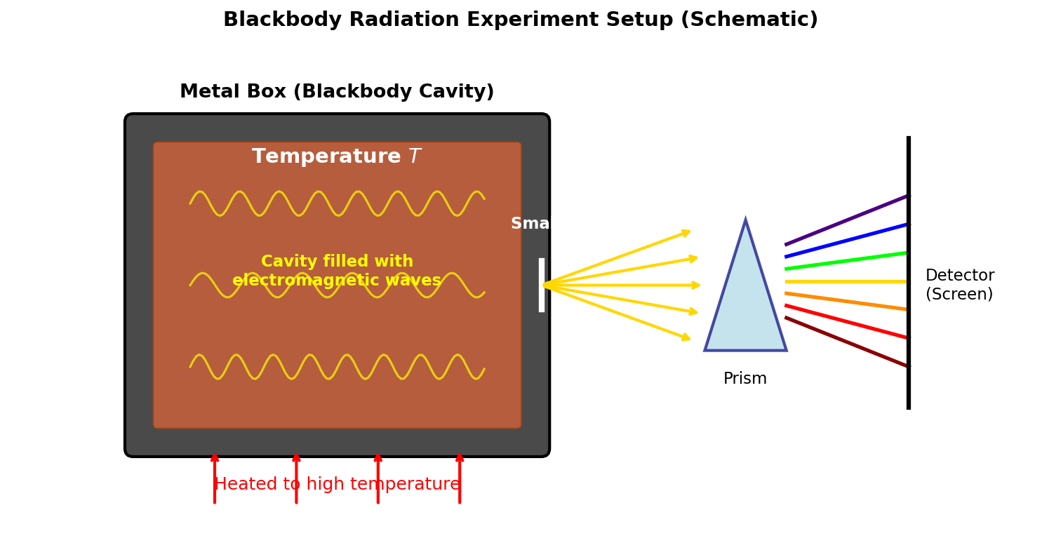
Fig. 1.1: Black-body radiation experimental setup. The interior of a metal box (black-body cavity) heated to high temperature is filled with electromagnetic waves. Light leaking through a small hole is dispersed by a prism, and the energy distribution as a function of frequency is measured.
⚪ Mei: So once you fix the temperature, the intensity of each color of light is determined.
🟡 Lina: Right. The experimental data had been precisely measured by the end of the 19th century. The problem was that calculations based on classical physics didn't match the experimental results at all.
🔵 Kai: How did they disagree?
🟡 Lina: When calculated using classical physics (Newtonian mechanics + Maxwell's electromagnetism + statistical mechanics), the radiated energy increases without bound as frequency increases. It diverges to infinity in the ultraviolet region. This is called the ultraviolet catastrophe.
🔵 Kai: Infinity!? That's clearly wrong, isn't it?
🟡 Lina: In experiments, the energy peaks at a certain frequency and then decreases properly. The theory predicts infinity while experiments show finite values. This isn't a matter of "errors after the decimal point"—it indicated a fundamental flaw in the framework of classical physics.
Planck's Quantum Hypothesis — Energy Comes in Discrete Chunks¶
🟡 Lina: The person who tackled this problem was the German physicist Max Planck. It was the year 1900.
🔵 Kai: How did he solve it?
🟡 Lina: Planck first found a mathematical formula that fit the experimental data. Then, when he tried to derive that formula theoretically, he realized he had to make a tremendous assumption.
⚪ Mei: A tremendous assumption?
🟡 Lina: Here it is:
The energy of a mode (oscillator) vibrating at frequency \(\nu\)—that is, each individual "vibration pattern" oscillating at a specific frequency—cannot take continuous values. It can only take values that are integer multiples of \(h\nu\).
In other words, the energy that a mode of frequency \(\nu\) can possess is limited to the discrete values \(0,\; h\nu,\; 2h\nu,\; 3h\nu,\; \ldots\) Intermediate values do not exist.
🔵 Kai: Wait, energy isn't continuous!?
🟡 Lina: The equation that appears here is the very first equation of quantum mechanics.
- \(E\): energy
- \(n\): a non-negative integer (\(0, 1, 2, \ldots\))
- \(h\): Planck's constant. One of the fundamental constants of nature
- \(\nu\) (the Greek letter "nu"): the frequency of light. A quantity corresponding to the color of light—higher frequency corresponds to violet or blue, lower frequency to red
⚪ Mei: The value of \(h\) is incredibly small. \(10^{-34}\)...
🟡 Lina: Yes. Because this value is so small, we don't notice that energy is "discrete" at everyday scales. Imagine a staircase. From far away it looks like a smooth ramp, but up close you can see each individual step. Planck's discovery was that the "ramp" of energy is actually a "staircase." Take a look at Fig. 1.2 "Comparison of the classical picture of energy (a continuous ramp) and the quantum picture (discrete steps)".
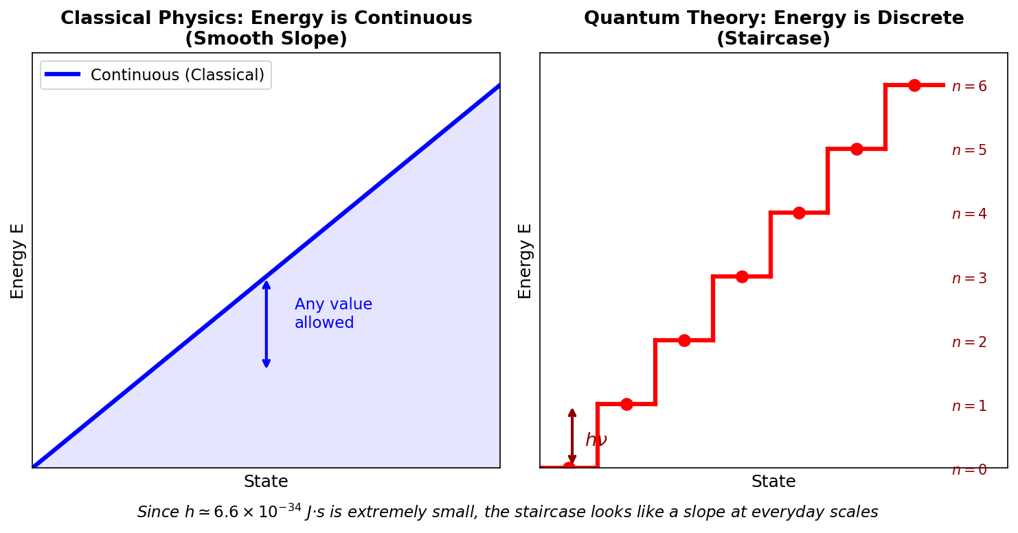
Fig. 1.2: Comparison of the classical picture of energy (a continuous ramp) and the quantum picture (discrete steps). Because \(h\) is extremely small, the step height is invisible at everyday scales, making it look like a smooth ramp.
🔵 Kai: I see... But why does making energy "discrete" resolve the ultraviolet catastrophe?
Why Discreteness Resolves the Ultraviolet Catastrophe¶
🟡 Lina: Good question. The key is the "thermal fluctuation energy" available to a system at temperature \(T\). Here we'll borrow a concept from statistical mechanics. Statistical mechanics is a field that treats the behavior of systems with many particles in thermal motion probabilistically. You don't cover it in detail in high school, but all we need now is one conclusion:
The typical energy of a single vibrational mode (a single frequency of light) in an environment at temperature \(T\) is on the order of \(k_B T\).
Here \(k_B \simeq 1.38 \times 10^{-23}\;\mathrm{J/K}\) is a natural constant called the Boltzmann constant, which serves as a bridge between "temperature" and "energy." The higher the temperature, the larger \(k_B T\) becomes, and the more energy is distributed to each mode—intuitively, "hotter means more vigorous vibration."
🔵 Kai: How large is \(k_B T\) specifically?
🟡 Lina: At room temperature (\(T \simeq 300\;\mathrm{K}\)), \(k_B T \simeq 4.1 \times 10^{-21}\;\mathrm{J} \simeq 0.026\;\mathrm{eV}\). The \(\mathrm{eV}\) (electron volt) is a unit of energy commonly used in atomic physics, where \(1\;\mathrm{eV} = 1.602 \times 10^{-19}\;\mathrm{J}\)—corresponding to the energy gained by a single electron accelerated through a potential difference of 1 V. This is "the benchmark for the thermal energy distributed to a single vibrational mode." The rigorous proof of why it's exactly \(k_B T\) is left to statistical mechanics textbooks, but intuitively, "temperature is a measure of the average kinetic energy of molecules," so the energy distributed to each mode is also proportional to temperature—that's \(k_B T\).
🔵 Kai: \(k_B T\) as the benchmark for thermal fluctuation energy... So regardless of frequency, every mode gets the same \(k_B T\)?
🟡 Lina: That is precisely the claim of classical physics. Every mode receives an equal share of approximately \(k_B T\) of energy—this is called the equipartition theorem. To be precise, it's "\(\frac{1}{2}k_BT\) per degree of freedom," and each mode of light has 2 degrees of freedom (oscillations of the electric and magnetic fields), giving a total of \(k_BT\). For now, just remember "each mode gets \(k_BT\)." In Fig. 1.3 "Comparison of equipartition and quantum theory", I've visually compared classical equipartition with quantum suppression. The left shows the classical case (equal \(k_BT\) distributed to all modes), and the right shows the quantum case (high-frequency modes become "frozen").
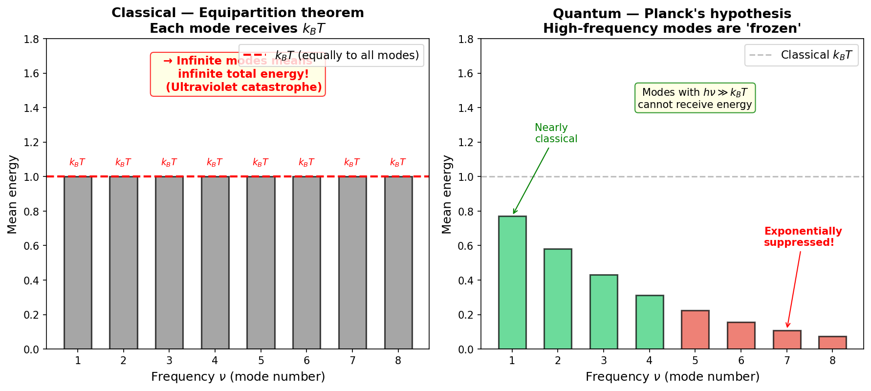
Fig. 1.3: Comparison of equipartition and quantum theory. Left: In classical equipartition, energy \(k_BT\) is uniformly distributed to all modes, and since the number of modes is infinite, the total energy diverges. Right: In Planck's quantum hypothesis, high-frequency modes with \(h\nu \gg k_BT\) cannot receive energy and are "frozen," so the total energy remains finite.
🔵 Kai: How many modes are there?
🟡 Lina: To answer that, let's first visualize "modes" concretely. Think of a guitar string. Both ends of the string are fixed, so only vibration patterns that fit exactly within the string's length can exist—half-wavelengths fitting 1, 2, 3 times... in discrete steps. These are the "modes" in one dimension.
🔵 Kai: I see, only waves that fit within the string length are allowed.
🟡 Lina: Light inside a box works the same way—only vibration patterns that fit between the walls are allowed. However, the box is three-dimensional, so there are combinations of vibration patterns in three directions: length, width, and depth. In one dimension, you just count "integer points on a number line," but in three dimensions, you count "lattice points in space." The vibration patterns in each direction are labeled by integers (1, 2, 3, ...), so each combination \((n_x, n_y, n_z)\) corresponds to one mode.
🔵 Kai: So each combination of three integers corresponds to a single vibration pattern.
🟡 Lina: Right. For a one-dimensional string, the vibration pattern number \(n\) was directly proportional to the frequency. In a three-dimensional box, the vibration pattern numbers \(n_x, n_y, n_z\) in each direction independently contribute to the frequency. In one dimension, the condition that "\(n\) half-wavelengths fit within the string length" made the frequency proportional to \(n\). In a three-dimensional box, this condition is imposed independently in each direction, so the frequency component in the \(x\) direction is \(\nu_x \propto n_x\), in the \(y\) direction \(\nu_y \propto n_y\), and in the \(z\) direction \(\nu_z \propto n_z\).
🔵 Kai: I understand the frequency in each direction. But how is the overall frequency determined? Do you simply add them?
🟡 Lina: Good question. Using \(\nu_x, \nu_y, \nu_z\) that I wrote as "\(x\)-direction frequency component \(\nu_x \propto n_x\)" and so on, the overall frequency is determined by \(\nu = \sqrt{\nu_x^2 + \nu_y^2 + \nu_z^2}\)—exactly the same structure as finding the distance from the origin to the point \((\nu_x, \nu_y, \nu_z)\) in three-dimensional space using the Pythagorean theorem. Why it's the square root of the sum of squares follows from the wave equation, which we'll cover in detail in later chapters. Intuitively, for a one-dimensional string, the frequency was determined by the condition "n half-wavelengths fit within the string length." In a three-dimensional box, this condition is imposed independently in the \(x\), \(y\), and \(z\) directions. When you solve the wave equation, the overall frequency is composed from the frequency components in each direction via the "3D Pythagorean theorem"—exactly the same structure as finding the diagonal length of a rectangular box from its three sides. For now, just accept that "this is the result." So "the number of modes with frequency \(\nu\) or less" corresponds to the number of lattice points inside a sphere of radius \(\propto \nu\), where we regard the vibration pattern numbers \((n_x, n_y, n_z)\) in each direction as coordinates.
⚪ Mei: So the frequency problem transforms into a geometry problem of "counting lattice points inside a sphere in 3D space."
🟡 Lina: Exactly. The lattice points are spaced 1 apart in each direction, so their count is approximately equal to the volume of the sphere (imagine one lattice point per small cube of side 1. Strictly speaking, there's some discrepancy near the sphere's surface, but the larger the radius, the more negligible this error becomes). However, since the vibration pattern numbers \(n_x, n_y, n_z\) take only positive integers (\(1, 2, 3, \ldots\)), we count only the "first octant"—that is, the region where \(n_x > 0,\; n_y > 0,\; n_z > 0\). This corresponds to \(1/8\) of the sphere's volume. Furthermore, light has two mutually perpendicular polarization directions, so even for the same vibration pattern there are 2 polarization choices, doubling the mode count. Since the sphere's volume is proportional to the cube of its radius, writing the proportionality constant (including the \(1/8\) and polarization factor of 2) as \(C\), the "total number of modes with frequency \(\nu\) or less" \(N(\nu)\) grows approximately as \(N(\nu) = C\nu^3\), proportional to \(\nu^3\).
🔵 Kai: \(N(\nu) \propto \nu^3\)... so if the frequency doubles, the number of modes becomes \(2^3 = 8\) times larger. That grows incredibly fast. But the ultraviolet catastrophe is about "how many modes are concentrated near a given frequency," right? It seems like we need the density per frequency, not the total count...
🟡 Lina: Exactly right. From here we find "the number of modes per unit frequency near frequency \(\nu\)"—which we call the mode density. The image of mode density is "how many new modes appear when you advance the frequency scale by a tiny bit." For example, it's like counting "how many stations are between 80 MHz and 81 MHz" on the FM radio band—mode density is the continuous version of that. Mathematically, it's the number of modes \(\Delta N\) that appear when \(\nu\) increases by \(\Delta\nu\), divided by \(\Delta\nu\): \(\Delta N / \Delta\nu\). When \(\Delta\nu\) becomes infinitesimally small, this is exactly the derivative \(dN/d\nu\) from high school math. From our earlier discussion, we can write \(N(\nu) = C\nu^3\) (\(C\) is a constant combining the box volume, the polarization factor of 2, the \(1/8\) for counting only positive integers, etc.—we don't need its specific value now). Differentiating with respect to \(\nu\) gives \(dN/d\nu = 3C\nu^2\)—so the mode density is proportional to \(\nu^2\).
⚪ Mei: Differentiating \(\nu^3\) gives \(3\nu^2\)—so the mode density grows as \(\nu^2\).
🟡 Lina: According to the equipartition theorem, each mode receives \(k_BT\) of energy, so the number of modes in the small interval from frequency \(\nu\) to \(\nu + d\nu\) is "mode density \(\times\) small width \(d\nu\)," that is, proportional to \(3C\nu^2\,d\nu\). Each receives \(k_BT\) of energy, so the energy in this interval is proportional to \(\nu^2 \cdot k_BT\,d\nu\). Summing this over all frequencies—that is, the integral \(\int_0^\infty \nu^2 \cdot k_BT\,d\nu\) proportional to the total radiation energy of the box.
🔵 Kai: Summing everything up with an integral... Does this converge?
🟡 Lina: Here, \(\int_0^R \nu^2\,d\nu\) uses the formula \(\int x^n\,dx = x^{n+1}/(n+1)\) from high school with \(n = 2\), giving \(\nu^3/3\) evaluated from \(0\) to \(R\), which is \(R^3/3\). As the upper limit \(R\) grows larger and larger, the value increases without bound, diverging to infinity as \(R \to \infty\)—this is the mathematical essence of the ultraviolet catastrophe.
⚪ Mei: So because the number of modes increases without limit with frequency, and each mode receives the same \(k_BT\), the total energy diverges.
🟡 Lina: Exactly. If you distribute \(k_B T\) to every mode, the total energy diverges—that's the ultraviolet catastrophe. In Fig. 1.4 "Mode counting and the mechanism of the ultraviolet catastrophe", I've illustrated this mechanism. The left side shows how to count modes using lattice points, and the right side shows the difference between classical and quantum energy densities.
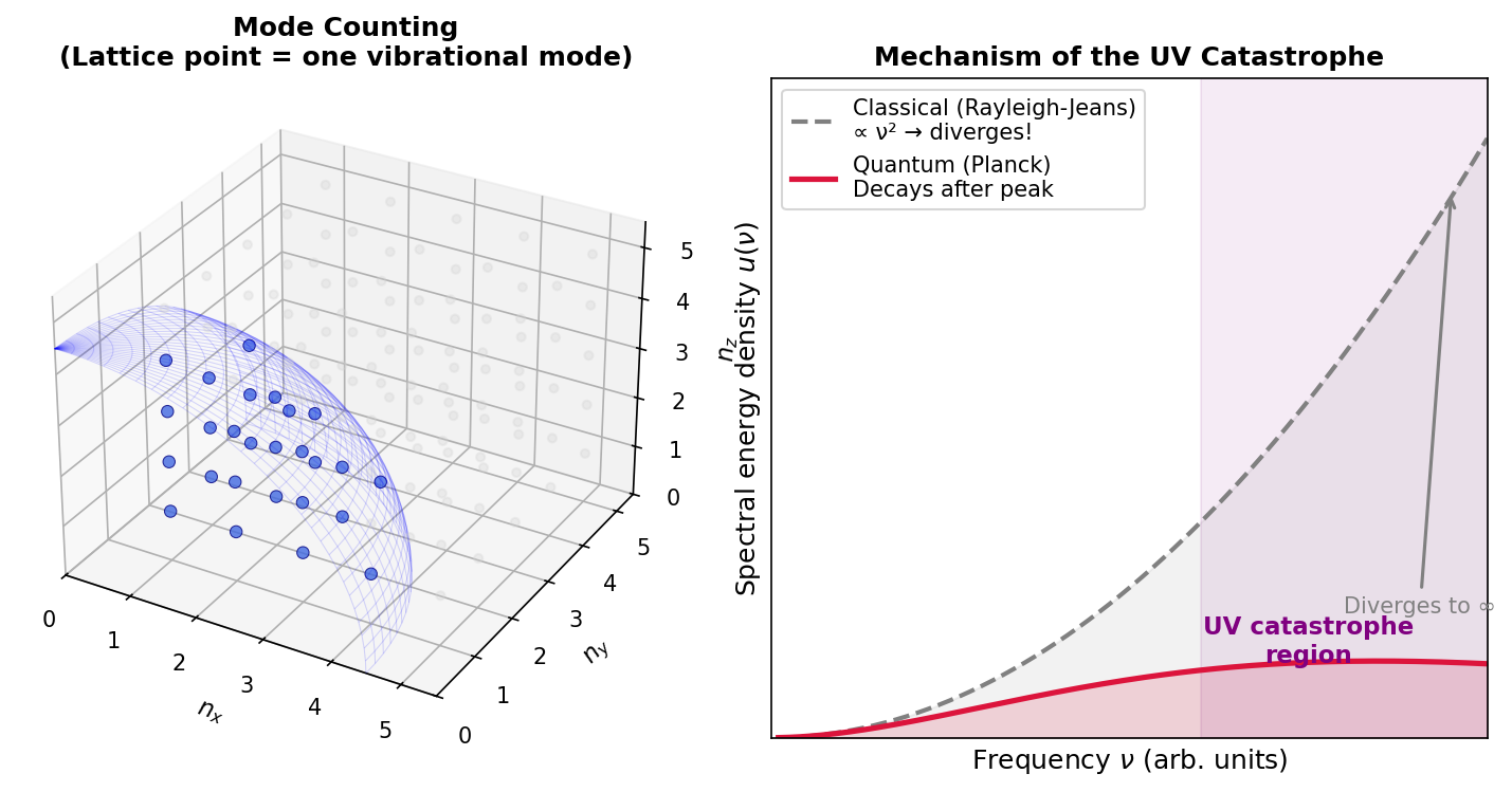
Fig. 1.4: Mode counting and the mechanism of the ultraviolet catastrophe. Left: Vibrational modes in a box are labeled by integer triples \((n_x, n_y, n_z)\), and the number of modes with frequency \(\nu\) or less corresponds to the number of lattice points inside a sphere of radius \(\propto \nu\). Right: In classical theory (gray dashed line), all modes receive \(k_BT\) uniformly and the energy diverges at high frequencies, but in Planck's quantum theory (red solid line), the high-frequency side is exponentially suppressed.
🔵 Kai: From what we discussed earlier, the number of modes grows proportional to \(\nu^3\) without limit. If you give each one \(k_B T\), it certainly diverges... How does Planck's hypothesis change things?
🟡 Lina: With Planck's quantum hypothesis, the "every mode gets \(k_B T\)" rule changes. A mode of frequency \(\nu\) needs at least one energy quantum \(h\nu\) to be excited, but the available "money" (thermal energy) is only \(k_B T\). If \(h\nu \gg k_B T\), you can't even buy a single ticket costing \(h\nu\).
In statistical mechanics there's an important law called the Boltzmann distribution. It tells us "at temperature \(T\), how likely is a state with energy \(E\) to be realized":
The symbol \(\propto\) (read "proportional to") means "is proportional to." So "probability \(\propto\) something" means "the probability is proportional to something." To give an intuitive reason for why it's an exponential function: "when you need to overcome several independent barriers, the probability of passing each one multiplies"—in high school probability you learned that "the probability of independent events occurring simultaneously is the product of their individual probabilities." For example, if the probability of passing one barrier is \(p\), then the probability of passing \(n\) barriers is \(p^n\). This decreases rapidly as \(n\) increases. Since \(p^n = e^{n \ln p}\), it decreases exponentially with the number of barriers \(n\)—this is the essence of the Boltzmann distribution's \(e^{-E/k_BT}\). The energy \(E\) corresponds to "the number of barriers to overcome," and \(k_BT\) corresponds to "the height of one barrier" (the same logic applies for continuous energy, thought of as the limit of infinitely fine steps).
🔵 Kai: Ah, the product of independent events becomes an exponential function. I didn't expect probability multiplication to show up here.
🟡 Lina: Think of it as: the higher you go on the staircase, the fewer "people" can reach there, dropping off rapidly. Thermal energy \(k_B T\) corresponds to "the stamina for one step," and the larger the required energy \(E\) is compared to that, the more drastically the probability of reaching it drops. Mathematically, "higher energy states are less likely to be realized"—and not just "less likely," but the probability drops exponentially rapidly. For example, if \(E = 3k_BT\), the probability is \(e^{-3} \approx 0.05\) (about 5%); if \(E = 10k_BT\), it's \(e^{-10} \approx 0.00005\) (essentially zero). So modes with \(h\nu \gg k_B T\) are effectively never excited at all.
🔵 Kai: Let me see... when \(h\nu\) is much larger than \(k_B T\), the exponent in \(e^{-h\nu/k_B T}\) becomes a large negative number, so it's nearly zero. So high-frequency modes "exist but effectively can't hold any energy"? But conversely, what about low-frequency modes? If \(h\nu\) is much smaller than \(k_BT\), are they excited normally?
🟡 Lina: Exactly. Low-frequency modes can hold \(k_BT\) of energy just like in the classical case. Take a look at Fig. 1.5 "Boltzmann distribution and quantum energy suppression. Left: The Boltzmann distribution \(e^{-E/k_BT}\)". The left graph shows the Boltzmann distribution itself, where you can see that the probability drops dramatically once the energy exceeds \(k_BT\). The right graph shows how the average energy of each vibrational mode changes with frequency.
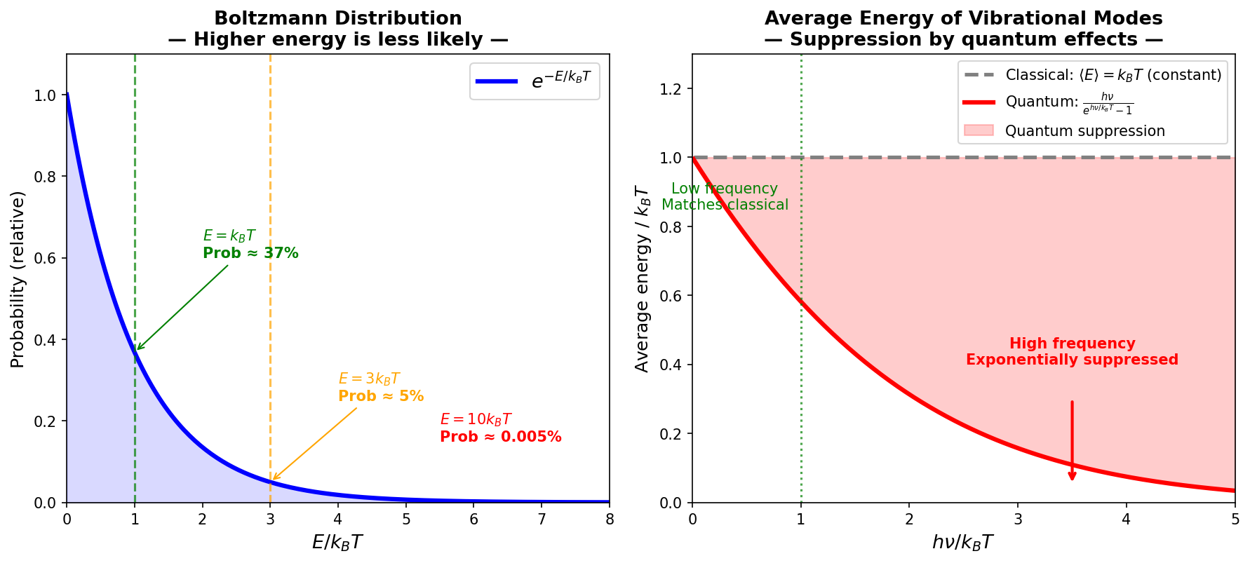
Fig. 1.5: Boltzmann distribution and quantum energy suppression. Left: The Boltzmann distribution \(e^{-E/k_BT}\) — the probability of higher energy states decreases exponentially. Right: Comparison of average energy of vibrational modes — classically all modes receive \(k_BT\) (gray dashed line), but in quantum theory the average energy is exponentially suppressed in the \(h\nu \gg k_BT\) region (red solid line).
🟡 Lina: Let's use the Boltzmann distribution to calculate "the average energy of a mode that can only take energies \(0, h\nu, 2h\nu, \ldots\)." I'll just show the approach. The probability of each energy \(nh\nu\) being realized is proportional to \(e^{-nh\nu/k_BT}\), so the average energy is "the sum of (each energy) × (its probability)" divided by "the sum of probabilities"—we write this as \(\langle E \rangle\) (the angle brackets \(\langle\;\rangle\) denote "average"). That is,
Here \(\sum_{n=0}^{\infty}\) (sigma notation) means "substitute \(n = 0, 1, 2, \ldots\) in order and add them all up"—so the denominator is \(e^{0} + e^{-h\nu/k_BT} + e^{-2h\nu/k_BT} + \cdots\).
🔵 Kai: Adding infinitely many terms? Doesn't it diverge?
🟡 Lina: Good question. Setting \(x = e^{-h\nu/k_BT}\), we have \(0 < x < 1\), so the denominator becomes a geometric series \(1 + x + x^2 + \cdots\). You've seen this sum in high school—if \(S = 1 + x + x^2 + \cdots\), multiply both sides by \(x\) to get \(xS = x + x^2 + x^3 + \cdots\). Subtracting gives \(S - xS = 1\), so \(S = 1/(1-x)\). Since \(|x| < 1\), each term gets progressively smaller and the sum converges to a finite value.
⚪ Mei: The denominator is \(1/(1-x)\). What about the numerator?
🟡 Lina: The numerator is \(\sum_{n=0}^\infty nh\nu \cdot x^n = 0 \cdot x^0 + 1 \cdot h\nu \cdot x + 2h\nu \cdot x^2 + \cdots\), but the \(n = 0\) term is zero so it vanishes, leaving \(h\nu \cdot x(1 + 2x + 3x^2 + \cdots)\). Here we use a technique. We want to find the sum of the series \(1 + 2x + 3x^2 + \cdots\). Actually, it can be found simply by differentiating the geometric series sum \(S = 1 + x + x^2 + \cdots = 1/(1-x)\) with respect to \(x\). Differentiating the left side term by term gives \(dS/dx = 0 + 1 + 2x + 3x^2 + \cdots = 1 + 2x + 3x^2 + \cdots\)—exactly the series we wanted (the constant term \(1\) differentiates to zero and vanishes). Differentiating the right side gives \(d[1/(1-x)]/dx = 1/(1-x)^2\). So we obtain \(1 + 2x + 3x^2 + \cdots = 1/(1-x)^2\). You might wonder "is it valid to differentiate an infinite sum term by term?"—when \(|x| < 1\) and each term gets progressively smaller so the sum converges to a finite value, this operation is permitted (the rigorous proof is left to university mathematics).
🔵 Kai: Can we verify this with a specific number?
🟡 Lina: Let's check with \(x = 1/2\): the right side is \(1/(1 - 1/2)^2 = 4\). The left side is \(1 + 2 \cdot (1/2) + 3 \cdot (1/4) + 4 \cdot (1/8) + \cdots = 1 + 1 + 0.75 + 0.5 + \cdots\), and adding these up, it indeed approaches 4. Using this, the numerator is \(h\nu \cdot x/(1-x)^2\). Since the denominator was \(1/(1-x)\), the average energy is
Substituting back \(x = e^{-h\nu/k_BT}\) gives \(1 - x = 1 - e^{-h\nu/k_BT}\), so
(the last equality comes from multiplying numerator and denominator by \(e^{h\nu/k_BT}\)).
⚪ Mei: That's a clean formula. So this is Planck's average energy formula.
🟡 Lina: Yes. Let's check the behavior of this formula in two limits.
- When \(h\nu \ll k_B T\) (low frequency): Setting \(\xi = h\nu/k_B T \ll 1\), we can approximate \(e^\xi \approx 1 + \xi\), so \(e^{h\nu/k_B T} - 1 \simeq h\nu / k_B T\), giving \(\langle E \rangle \simeq k_B T\) (agreeing with the classical result)
- When \(h\nu \gg k_B T\) (high frequency): \(e^{h\nu/k_BT} \gg 1\), so the \(-1\) in the denominator is negligible and \(\langle E \rangle \simeq h\nu\, e^{-h\nu / k_B T}\), which is exponentially suppressed
⚪ Mei: I see. The high-frequency side is exponentially suppressed by \(e^{-h\nu / k_B T}\), so it doesn't diverge to infinity.
🔵 Kai: Oh, I get it! The low-frequency side behaves classically at \(k_B T\), but only the high-frequency side enters the "ticket is too expensive to buy" state, so the total stays finite... But wait a moment. What happens if you raise the temperature? If \(k_BT\) gets larger, won't higher frequency modes become excited too, shifting the spectrum peak to higher frequencies?
🟡 Lina: Exactly right. When temperature increases, \(k_BT\) gets larger, so the upper limit of frequencies where "the ticket is affordable" rises, and the peak shifts to higher frequencies. But no matter how high the temperature, the region \(h\nu \gg k_BT\) always exists and is exponentially suppressed there—so the total energy always remains finite. In other words, by making energy "discrete," high-frequency modes become difficult to excite through thermal fluctuations. This resolves the ultraviolet catastrophe. The classical "equipartition theorem" breaks down, and Planck's formula matches experiments perfectly. Look at Fig. 1.6 "Comparison of black-body radiation energy density". You can see that while the classical prediction (Rayleigh-Jeans) diverges at high frequencies, Planck's formula decays exponentially beyond the peak. The figure also shows spectra at multiple temperatures—you can see that the peak shifts to higher frequencies at higher temperatures. This is an empirical rule called Wien's displacement law, which emerges naturally from Planck's formula.
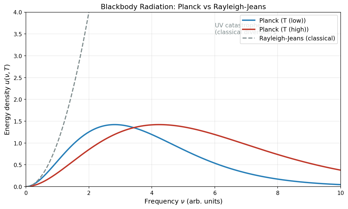
Fig. 1.6: Comparison of black-body radiation energy density. The classical Rayleigh-Jeans prediction (gray dotted line) diverges at high frequencies, while Planck's formula (solid lines) decays exponentially beyond the peak. The peak shifts to higher frequencies at higher temperatures (Wien's displacement law).
🔵 Kai: Amazing! A single assumption solves it. But... you've only assumed "it's discrete"—we still don't know why it's discrete, right?
🟡 Lina: You're hitting on a great point. In fact, Planck himself felt the same way. He thought this assumption was a "mathematical trick." A convenient device to make the calculation work—he didn't actually believe that energy was truly discrete. He later said it was "an act of desperation."
⚪ Mei: So Planck didn't realize he had started a revolution in physics.
🟡 Lina: That's right. The person who took Planck's hypothesis seriously and pushed it further was—Einstein, who appears next.
✅ Comprehension Check: How does the extremely small value of Planck's constant \(h\) relate to the fact that the "discreteness" of energy is not observed in everyday life?
Answer
Since \(h \simeq 6.626 \times 10^{-34}\;\mathrm{J \cdot s}\) is extremely small, at everyday scales the minimum energy unit \(h\nu\) becomes negligibly tiny. Therefore, the staircase-like energy appears as a smooth continuous quantity, and quantum effects go unnoticed.
✅ Comprehension Check: What is the ultraviolet catastrophe? Also, describe in one sentence each how Planck's quantum hypothesis resolves it.
Answer
Ultraviolet catastrophe: The problem that when black-body radiation is calculated using classical physics, the radiated energy diverges to infinity at high frequencies. Resolution: By assuming that energy can only take integer multiples of \(h\nu\), photons at high frequencies have too much energy per quantum to be easily radiated, naturally suppressing the high-frequency side.
📝 Exercises:
- Calculation to appreciate the smallness of Planck's constant → Problem B-1. Appreciating the Smallness of Planck's Constant
1.3 Crisis ②: The Mystery of the Photoelectric Effect¶
Light Hits Metal and Electrons Fly Out — But Something Strange Happens¶
🟡 Lina: The second crisis is the "photoelectric effect." This phenomenon was discovered by Hertz in 1887—when light is shone on the surface of a metal, electrons fly out from inside the metal.
🔵 Kai: Like knocking electrons out with light?
🟡 Lina: Yes. The phenomenon itself was known, but when examined in detail, strange properties were found that classical physics absolutely could not explain. Let me list four puzzles (Table 1.1 "Four puzzles of the photoelectric effect and contradictions with classical predictions").
Table 1.1: Four puzzles of the photoelectric effect and contradictions with classical predictions
| Puzzle | Experimental fact | Classical wave prediction |
|---|---|---|
| ① Existence of a threshold | Below a certain frequency, no electrons emerge no matter how intense the light | Intense light should eject them |
| ② Independent of intensity | Making light brighter doesn't change the energy of each ejected electron | Brighter light should give more energy |
| ③ Proportional to frequency | Higher light frequency gives electrons more energy | Should be determined by intensity |
| ④ Instantaneous response | Electrons fly out the instant light hits | Energy accumulation should take time |
🔵 Kai: Everything is the opposite of the classical prediction!
🟡 Lina: That's right. In the classical wave theory, the energy of light is determined by its amplitude (brightness). The wave gradually transfers energy to the electron, and when enough has accumulated, the electron flies out—so shining bright light should accumulate energy faster and eject electrons. But the experimental results say that color (frequency), not brightness, is what matters.
⚪ Mei: Increasing brightness doesn't change electron energy, but changing color does... The wave theory simply can't explain this.
Einstein's Light Quantum Hypothesis — Light Is Also a Particle¶
🟡 Lina: This is where Albert Einstein enters the picture. In 1905—the same year he published special relativity—he wrote another revolutionary paper.
🔵 Kai: Two in the same year!?
🟡 Lina: Einstein pushed Planck's idea of "energy packets" further. Planck had said "the energy of light takes discrete values," but Einstein made an even bolder claim:
Light itself is a collection of particles, each carrying energy \(h\nu\).
In other words, light is not a continuous wave but something like "packets (parcels) of energy" flying through space. These light particles are today called photons.
🔵 Kai: Light is a particle!? But wasn't light a wave? Interference, diffraction...
🟡 Lina: That's a perfectly valid question. 19th-century physics established that light is a wave through Young's double-slit experiment, where interference fringes were observed. And yet "it is both a wave and a particle"—this "wave-particle duality" will be covered in detail in the next chapter. For now, let's focus on how Einstein's hypothesis explains the photoelectric effect.
The Hail Analogy — Why Color Is What Matters¶
🟡 Lina: To intuitively understand Einstein's explanation, let me use the hail analogy.
What determines whether a car hood gets dented isn't the total amount of hail falling, but the size of each individual hailstone, right? Even if an enormous amount of hail falls, if each stone is as small as a grain of sand, the hood won't dent. Conversely, even with just a few hailstones, if each one is golf-ball-sized, a single hit will dent it.
🔵 Kai: Ah, I see! So light works the same way?
🟡 Lina: Exactly. No matter how intense the light (= many photons), if each photon's energy is small (= low frequency), electrons won't be knocked out of the atom. Conversely, even weak light, if the frequency is high enough, has large energy per photon and electrons will fly out. Take a look at Fig. 1.7 "Understanding the photoelectric effect through the hail analogy".
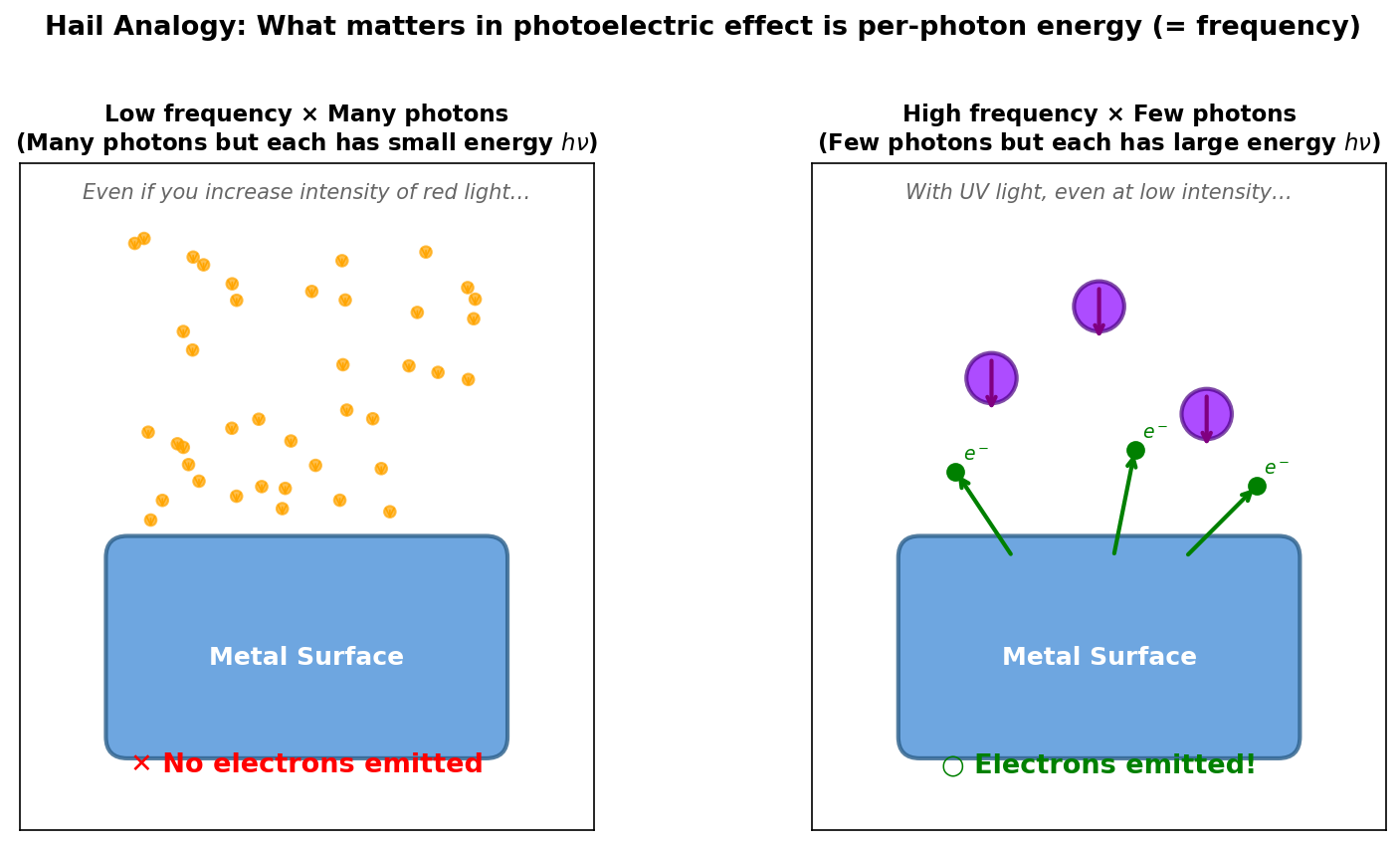
Fig. 1.7: Understanding the photoelectric effect through the hail analogy. Left: Low-frequency (red light) photons have small energy \(h\nu\), so no matter how many hit the surface, they cannot knock out electrons. Right: High-frequency (ultraviolet) photons each carry large energy, so even a small number can knock out electrons. What matters in the photoelectric effect is not the intensity of light (number of photons) but its color (frequency).
⚪ Mei: So color is what matters, not intensity. Intensity only corresponds to the number of photons.
The Photoelectric Equation¶
🟡 Lina: Let me write this quantitatively. Electrons inside a metal are bound by the positive charges of surrounding nuclei—like being inside a "room surrounded by walls." The minimum energy needed to climb over this wall and get out is written as \(W\) and called the work function. \(W\) comes from the initial letter of "Work"—meaning the minimum energy needed for the "work" of tearing an electron free. The condition for the photoelectric effect to occur is
and when this condition is met, the kinetic energy \(K\) of the ejected electron is
🔵 Kai: The energy \(h\nu\) carried by one photon minus the energy \(W\) used to tear the electron free equals the electron's kinetic energy... That's simple! But what if two photons hit simultaneously and their combined energy knocks the electron out?
🟡 Lina: Good question. With very intense laser light, a phenomenon called "multi-photon absorption" does occur. But in typical photoelectric effect experiments, the light intensity isn't that high, so the probability of two photons hitting the same electron nearly simultaneously is extremely low. The process where one photon delivers energy to one electron in a one-to-one interaction is overwhelmingly dominant, so equation (1.4) is sufficient. Now, looking at equation (1.4), all four puzzles can be explained (Table 1.2 "Einstein's light quantum hypothesis explains the photoelectric effect").
Table 1.2: Einstein's light quantum hypothesis explains the photoelectric effect
| Puzzle | Einstein's explanation |
|---|---|
| ① Threshold | If \(h\nu < W\), a single photon doesn't have enough energy to overcome the barrier, so no electron emerges |
| ② Intensity-independent | A single photon's energy is determined by \(h\nu\) and does not depend on the number of photons (= intensity) |
| ③ Proportional to frequency | From \(K = h\nu - W\), larger \(\nu\) gives larger \(K\) |
| ④ Instantaneous response | A single photon delivers energy to an electron instantaneously. No accumulation needed |
⚪ Mei: Everything explained by a single equation.
🟡 Lina: Look at Fig. 1.8 "Relationship between kinetic energy and frequency in the photoelectric effect". If you plot \(K\) against \(\nu\), you get a straight line with slope \(h\). The frequency where the line intersects \(K = 0\) is \(\nu_0 = W/h\), the threshold frequency—below this frequency, no electrons fly out no matter how intense the light. The threshold frequency (i.e., the intercept \(-W\)) varies depending on the type of metal, but the slope is always the same—this is one of the experimental methods for determining Planck's constant.
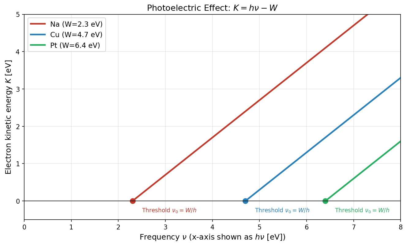
Fig. 1.8: Relationship between kinetic energy and frequency in the photoelectric effect. The linear relationship \(K = h\nu - W\) of electron kinetic energy in the photoelectric effect. The threshold \(\nu_0 = W/h\) differs by metal, but the slope is universally the same, giving Planck's constant \(h\). The point where the line crosses \(K = 0\) is the threshold frequency; below it, no electrons are ejected regardless of intensity.
🟡 Lina: Einstein received the Nobel Prize for this work. Not for relativity—for the theory of the photoelectric effect.
🔵 Kai: Wow! Not for relativity.
Einstein Is One of the Founders of Quantum Theory¶
🟡 Lina: There's something I want to emphasize here. Einstein is famous for later criticizing quantum mechanics—have you heard the phrase "God does not play dice"?
🔵 Kai: Oh, I've heard that.
🟡 Lina: But that came later. In 1905, Einstein was on the side that created quantum theory. Planck said "energy is discrete," and Einstein said "light itself is a particle." Furthermore, in 1917 he introduced the concept of "stimulated emission," which later became the principle behind lasers. Einstein is one of the founders of quantum theory—don't forget this. In later chapters, there will be a dramatic scene where this founder reappears as a critic.
⚪ Mei: Creating a theory himself, then later criticizing it... How dramatic.
✅ Comprehension Check: How does Einstein's light quantum hypothesis differ from Planck's quantum hypothesis? Describe the difference between their claims.
Answer
Planck claimed that "the energy of light at frequency \(\nu\) can only take values that are integer multiples of \(h\nu\)" (discretization of energy). Einstein, on the other hand, claimed that "light itself is a collection of particles (photons) each carrying energy \(h\nu\)." In other words, Einstein was more audacious in interpreting the discreteness not as a property of how light is emitted or absorbed, but as a property of light's very existence.
✅ Comprehension Check: In the photoelectric effect, explain using the concept of photons why the energy of ejected electrons doesn't change even when the "intensity" of light is increased.
Answer
The intensity of light corresponds to the number of photons. Each individual photon's energy is \(h\nu\) (determined by frequency), and increasing intensity doesn't change the energy per photon. Since knocking out an electron is the job of a single photon, the energy of the ejected electron \(K = h\nu - W\) does not depend on intensity.
📝 Exercises:
- Calculating work function and threshold frequency → Problem B-2. Work Function and Threshold Frequency
1.4 Crisis ③: The Problem of Atomic Stability¶
Rutherford's Atomic Model — A Solar System-like Atom¶
🟡 Lina: The third crisis is the problem of "atomic stability." You could say this was the most serious of all.
🔵 Kai: Atoms exist stably, don't they? What's the problem?
🟡 Lina: The problem is that "according to classical physics, atoms cannot exist stably." Let's first confirm the structure of the atom. In 1911, Ernest Rutherford revealed the structure of the atom through his famous gold foil experiment. The result was this—at the center of the atom is a small, heavy nucleus carrying positive charge, with negatively charged electrons orbiting around it. A solar system-like structure.
⚪ Mei: We learned that in high school too. But what's the specific scale?
🟡 Lina: According to experiments, the atomic radius is about \(10^{-10}\;\mathrm{m}\), while the nuclear radius is about \(10^{-15}\;\mathrm{m}\). The nucleus is only 1/100,000 the size of the whole atom. The electrons orbit far from the nucleus. Look at Fig. 1.9 "Rutherford's atomic model. A negatively charged electron (green) orbits in a circular path around a positively charged nucleus (red) at the center. The atomic radius is \(\sim 10^{-10}\) m while the nuclear radius is \(\sim 10^{-15}\) m".
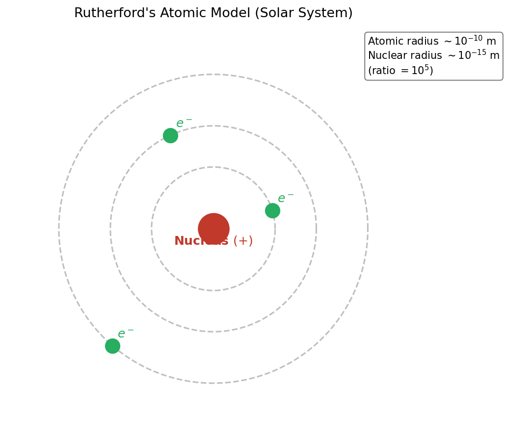
Fig. 1.9: Rutherford's atomic model. A negatively charged electron (green) orbits in a circular path around a positively charged nucleus (red) at the center. The atomic radius is \(\sim 10^{-10}\) m while the nuclear radius is \(\sim 10^{-15}\) m—overwhelmingly smaller. This model explains experimental facts but, as we'll see next, is incompatible with classical electromagnetism.
🔵 Kai: The solar system model is easy to understand. What could be the problem...
The Prediction of Classical Electromagnetism — Atoms Collapse Instantly¶
🟡 Lina: The problem lies in Maxwell's electromagnetism. According to this theory, an accelerating charge must radiate electromagnetic waves.
🔵 Kai: Circular motion is... accelerated motion, right? There's centripetal acceleration.
🟡 Lina: Exactly! An electron in circular motion always has centripetal acceleration, so according to Maxwell's theory, the electron must continuously radiate electromagnetic waves. Radiating electromagnetic waves means losing energy.
🔵 Kai: If it loses energy... what happens to the electron?
🟡 Lina: It spirals inward and falls into the nucleus. Classical electromagnetism has a formula (Larmor's formula) giving the "power radiated by an accelerating charge." Roughly speaking, when a charge \(e\) moves with acceleration \(a\), the radiated power (energy loss per unit time) is proportional to \(P \propto e^2 a^2 / c^3\). The electron in a hydrogen atom, at a distance \(r \sim 10^{-10}\;\mathrm{m}\) from the nucleus, experiences centripetal acceleration \(a \sim v^2/r\), so we can estimate the radiated power. Dividing the electron's total energy (\(\sim\) a few eV) by this power gives a collapse time of
—that is, it completes in about one hundred-billionth of a second. You can try the specific calculation in the exercises (the precise form of Larmor's formula will be given in the problem statement, so you don't need to memorize it now).
🔵 Kai: That's instantaneous! But in reality, atoms have existed stably for billions of years...
🟡 Lina: Right. According to classical physics, atoms cannot exist stably at all. Yet the atoms making up your body have existed without collapsing for billions of years. This is a clear contradiction. In Fig. 1.10 "Classical atom collapse through electromagnetic radiation", I've illustrated the electron spiraling inward.
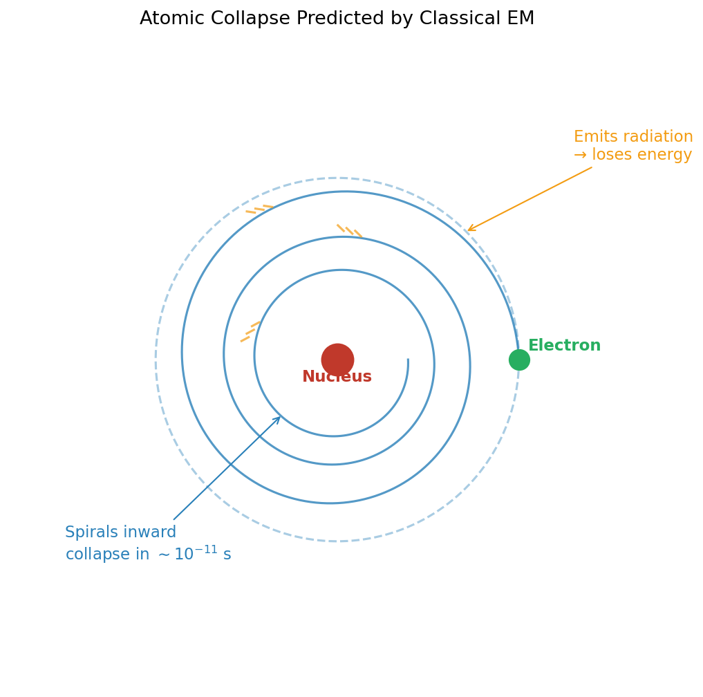
Fig. 1.10: Classical atom collapse through electromagnetic radiation. The collapse predicted by classical electromagnetism. The electron loses energy while radiating electromagnetic waves, spiraling into the nucleus. Collapse is completed in about \(10^{-11}\) seconds.
🔵 Kai: This is serious... If we accept both Newtonian mechanics and Maxwell's electromagnetism, atoms can't exist.
🟡 Lina: There's another problem. If the electron spirals inward, the frequency of electromagnetic waves radiated during the process should change continuously. This is because the orbital radius decreases continuously, so the electron's orbital frequency also changes continuously. However, when we examine light emitted by atoms experimentally, only specific frequencies of light are observed. The spectral lines are discrete.
⚪ Mei: It should change continuously, yet in reality it's discrete—another contradiction that classical physics cannot explain.
🟡 Lina: Exactly. Atomic stability and the discreteness of spectra—Bohr's model, which we'll see next, solved both mysteries simultaneously.
✅ Comprehension Check: State in 2 sentences or fewer why classical electromagnetism predicts that atoms cannot exist stably.
Answer
An electron in circular motion is undergoing accelerated motion, so according to Maxwell's electromagnetism it must continuously radiate electromagnetic waves and lose energy. As a result, the electron spirals inward and falls into the nucleus in about \(10^{-11}\) seconds.
📝 Exercises:
- Order-of-magnitude estimate of classical atomic collapse time → Problem M-3. Order-of-magnitude estimate of classical atomic collapse time
1.5 Bohr's Atomic Model and the Rydberg Formula¶
Atomic Spectra — The "Fingerprint" of Matter¶
🟡 Lina: Now, before getting into Bohr's model, let's look at the experimental facts in a bit more detail. When we disperse the light emitted by atoms with a prism, only specific frequencies of light appear as thin lines (emission lines). These are called the spectrum.
🔵 Kai: So not all colors come out like a rainbow—only specific colors?
🟡 Lina: Right. The spectrum has a pattern unique to each element, like a "fingerprint" of the substance. The hydrogen atom's spectrum is the simplest and shows a regular pattern.
In 1885, Balmer discovered that the spectral lines of hydrogen in the visible region follow a simple formula. This was later generalized into what's known as the Rydberg formula.
✅ Comprehension Check: What does it mean that an atom's spectrum is "discrete"? Also, how does this contradict the prediction of classical physics?
Answer
The light emitted by atoms does not contain all frequencies (colors) but only specific frequencies appearing as thin emission lines. In classical electromagnetism, since the orbital radius of a spiraling electron changes continuously, the frequency of radiated light should also change continuously, making discrete spectral lines inexplicable.
where - \(\lambda\): wavelength of the emitted light - \(R_\infty\): Rydberg constant. \(R_\infty \simeq 1.097 \times 10^7\;\mathrm{m^{-1}}\) - \(n, m\): positive integers (\(m > n\))
🔵 Kai: What happens when you plug in specific numbers for \(n\) and \(m\)?
🟡 Lina: Setting \(n = 1\) and \(m = 2, 3, 4, \ldots\) gives a series in the ultraviolet region. This is called the Lyman series. Setting \(n = 2\) and \(m = 3, 4, 5, \ldots\) gives a series in the visible region—the Balmer series.
⚪ Mei: The value of \(n\) determines the series, and varying \(m\) gives individual lines within that series.
🟡 Lina: Exactly. This formula reproduces the experimental data perfectly. But in 1885, nobody could explain why such a formula holds. What do the integers \(n\) and \(m\) mean? Why the form \(1/n^2\)? Bohr was the one who answered these questions.
Bohr's Three Postulates¶
🟡 Lina: In 1913, the Danish physicist Niels Bohr applied the quantum hypotheses of Planck and Einstein to the atom and proposed a bold model. It consists of three postulates.
Postulate 1: Existence of stationary states
Electrons can exist stably only when in specific orbits (stationary states), without radiating electromagnetic waves. The allowed orbits are discrete, and orbits in between do not exist.
🔵 Kai: Wait, he just declares "no radiation"? Doesn't that contradict Maxwell's theory?
🟡 Lina: It does contradict it. Bohr explicitly stated, as a postulate, that "in the atomic world, classical electromagnetism does not hold as-is." Bold, isn't it?
Postulate 2: Quantum condition
Only orbits where the electron's angular momentum \(L\) takes specific values are allowed. The reason for angular momentum is that the units of Planck's \(h\) are \(\mathrm{J \cdot s}\) (energy × time), which have the same dimensions as angular momentum. Let's verify—the dimensions of angular momentum \(L = mvr\) are \(\mathrm{kg \cdot (m/s) \cdot m} = \mathrm{kg \cdot m^2/s}\). Meanwhile, \(\mathrm{J \cdot s} = \mathrm{kg \cdot m^2/s^2 \cdot s} = \mathrm{kg \cdot m^2/s}\). They're indeed the same. So "if you're going to impose a quantum condition related to \(h\), angular momentum is the natural candidate."
🔵 Kai: Because the dimensions match, it's natural to impose the condition on angular momentum.
🟡 Lina: Angular momentum is a quantity representing the "momentum of rotation." In linear motion, momentum is expressed as \(mv\) (mass × speed)—you've seen this in high school physics. The momentum of rotational motion is represented by "momentum \(mv\) × radius of rotation \(r\)." The reason for multiplying by radius is that even at the same speed, a larger radius of rotation means it's "harder to stop the rotation"—for example, when spinning a stone on a string, the longer the string, the harder it is to stop. Even at the same speed, something rotating farther out has greater rotational momentum. Rotational momentum increases with "speed × radius." So for an object of mass \(m\) moving at speed \(v\) in a circular orbit of radius \(r\), we define \(L = mvr\). Bohr's condition is
Here \(\hbar\) (read "h-bar") \(= h / 2\pi\) is Planck's constant divided by \(2\pi\), also called the Dirac constant. You might wonder "why divide by \(2\pi\) instead of using \(h\) itself?"—this is deeply related to circular motion (one revolution \(= 2\pi\) radians, i.e., \(360°\)), and will become naturally understandable when we learn about de Broglie's matter waves in the next chapter. \(n\) is a positive integer called the quantum number. \(n = 0\) is not allowed—if the angular momentum were zero, the electron wouldn't be rotating and no orbit would exist.
🔵 Kai: I see, \(n = 0\) means "not rotating" so the electron would fall into the nucleus... But is a "non-rotating" state truly impossible in all cases? Could this get overturned later?
🟡 Lina: Good question. In the Bohr model, the premise is that "the electron travels in a circular orbit," so \(n = 0\) (no rotation) would make the orbital radius zero and the electron would overlap with the nucleus—the model wouldn't make sense. So within the framework of the Bohr model, \(n \geq 1\) is a logically correct restriction. However, as a preview, in later quantum mechanics, states with zero angular momentum are allowed—in that case the electron isn't "orbiting" but exists in a completely different way. We'll cover that in detail in later chapters. For now, let's proceed with \(n \geq 1\) within the Bohr model framework.
⚪ Mei: To summarize, the key point of Postulate 2 is "angular momentum can only take integer multiples of \(\hbar\)." Dividing the earlier value of \(h\) by \(2\pi\):
which, like \(h\), is extremely small.
Postulate 3: Frequency condition
When an electron "jumps" from an orbit with energy \(E_m\) to an orbit with energy \(E_n\) (\(E_m > E_n\)), light is emitted with a frequency corresponding to that energy difference.
⚪ Mei: Postulate 3 uses Planck's \(E = h\nu\). The energy difference becomes exactly the energy of one photon.
🔵 Kai: Planck → Einstein → Bohr—each person develops the previous person's idea. But what exactly does "jumping" look like...?
🟡 Lina: Good question. "Jumping" means moving instantaneously to another orbit without passing through intermediate states—completely different from the classical picture of "gradually moving." It's a picture unique to quantum theory. Look at Fig. 1.11 "Bohr's frequency condition". It illustrates how a photon is emitted when an electron jumps from a higher level to a lower one, with an energy corresponding to their difference. And since each combination of starting and ending points gives a different frequency of light, the spectral lines are discrete.
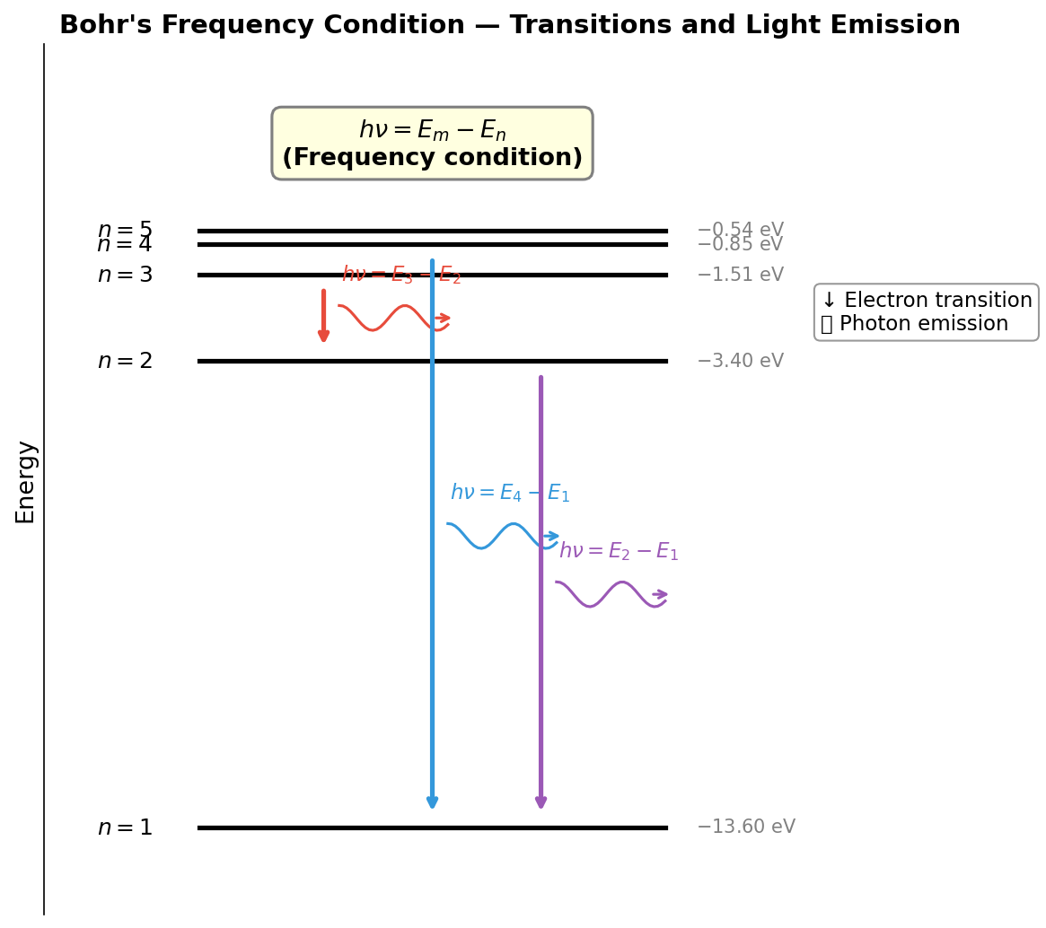
Fig. 1.11: Bohr's frequency condition. When an electron transitions from energy level \(E_m\) to \(E_n\) (\(m > n\)), a photon with energy \(h\nu\) equal to the energy difference \(E_m - E_n\) is emitted. Different combinations of starting and ending levels produce different frequencies of light, corresponding to discrete spectral lines.
🟡 Lina: For organization, let me compare the quantization ideas of the three physicists (Table 1.3 "Comparison of quantization ideas by Planck, Einstein, and Bohr").
Table 1.3: Comparison of quantization ideas by Planck, Einstein, and Bohr
| Physicist | What was quantized | Equation | Level of boldness |
|---|---|---|---|
| Planck (1900) | Energy of oscillators | \(E = nh\nu\) | Intended as a "mathematical trick" |
| Einstein (1905) | Light itself (photons) | \(E_{\text{photon}} = h\nu\) | Changed the very nature of light |
| Bohr (1913) | Electron orbits (angular momentum) | \(L = n\hbar\) | Partially abandoned classical electromagnetism |
🔵 Kai: It feels like they're getting progressively bolder. Mathematical trick → the nature of light → abandoning classical theory...
Derivation of the Hydrogen Atom Energy Levels¶
🟡 Lina: Now let's apply Bohr's postulates to the hydrogen atom and do the calculation explicitly. The hydrogen atom is the simplest atom, with a single proton (charge \(+e\)) as the nucleus, and a single electron (charge \(-e\), mass \(m_e\)) orbiting around it.
🔵 Kai: The simplest version of the solar system model.
🟡 Lina: Let's say the electron moves in a circular orbit of radius \(r\) at speed \(v\). The condition for circular motion is that the Coulomb force provides the centripetal force. In high school, you wrote Coulomb's law as \(F = kq_1q_2/r^2\). Here we'll use the standard notation in physics, rewriting the Coulomb constant \(k\) as \(k = 1/(4\pi\varepsilon_0)\). \(\varepsilon_0\) is a constant called the permittivity of free space (\(\varepsilon_0 \simeq 8.854 \times 10^{-12}\;\mathrm{F/m}\)), and writing the Coulomb constant \(k\) as \(k = 1/(4\pi\varepsilon_0)\) is just an alternative notation carrying the same information as \(k \simeq 8.99 \times 10^9\;\mathrm{N \cdot m^2/C^2}\). If you remember the value of \(k\) from high school, you can find \(\varepsilon_0 = 1/(4\pi k)\). In calculations you just substitute the numerical value of \(\varepsilon_0\), so don't worry about the meaning of the units \(\mathrm{F/m}\) for now. For the hydrogen atom, \(q_1 = +e\) (proton), \(q_2 = -e\) (electron), and the magnitude of the force is
The left side is the magnitude of the Coulomb force, the right side is the centripetal force \(m_e v^2 / r\).
⚪ Mei: The same structure as "gravitational force provides centripetal force" from high school physics. Just with Coulomb force instead of gravity.
🟡 Lina: Rearranging equation (1.10):
Next, we use the angular momentum quantum condition (Postulate 2). The angular momentum of circular motion is \(L = m_e v r\), so
Substituting \(v = n\hbar / (m_e r)\) from equation (1.12) into equation (1.11):
Multiplying both sides by \(r\) and solving:
🔵 Kai: The orbital radius is proportional to \(n^2\)! \(n = 1\) is the smallest orbit.
🟡 Lina: Right. In Fig. 1.12 "Allowed orbits in Bohr's atomic model" I've drawn the orbits for each quantum number. You can see how the orbital radius expands rapidly as \(n\) increases.
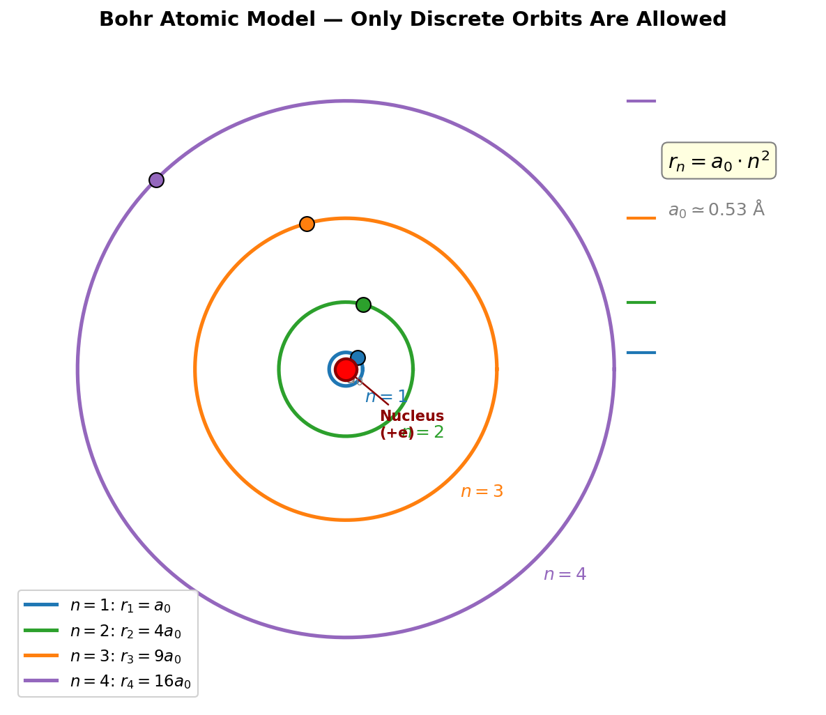
Fig. 1.12: Allowed orbits in Bohr's atomic model. From \(r_n = a_0 n^2\), the orbital radii for \(n = 1, 2, 3, 4\) are \(a_0, 4a_0, 9a_0, 16a_0\), expanding as the square. Intermediate radii are not allowed, and electrons can exist only on these discrete orbits.
🟡 Lina: The radius at \(n = 1\) is called the Bohr radius and written as \(a_0\).
⚪ Mei: About \(0.5 \times 10^{-10}\;\mathrm{m}\)... that matches the order of magnitude of atomic size!
🟡 Lina: Now let's find the energy. The total energy of the electron is the sum of kinetic energy and electrostatic potential energy (Coulomb potential energy). Let me review the concept of potential energy.
🔵 Kai: In high school, we learned potential energy as "\(mgh\) with the ground as reference," but what's the reference for an atom?
🟡 Lina: Good question. For atoms, we take "the state where the electron is infinitely far from the nucleus and no longer feels the attractive force" as the reference (zero). In outer space with no ground, we set "completely free state" as zero. Then, when two charges attracting each other approach to distance \(r\), the potential energy becomes \(-e^2/(4\pi\varepsilon_0 r)\). This is the negative of "the work done against the Coulomb attraction to separate the electron from distance \(r\) to infinity." The closer they are (attracted by the force), the lower the energy, so the sign is negative—the same structure as gravitational potential energy \(-GMm/r\).
⚪ Mei: Zero at infinity, and the more bound it is, the more negative—that's intuitively clear.
🟡 Lina: I'll leave the derivation details to the exercises, but for now remember that "when the force is proportional to \(1/r^2\), the work to separate from distance \(r\) to infinity is proportional to \(1/r\)." In high school math terms, the magnitude of the Coulomb force was \(F = e^2/(4\pi\varepsilon_0 r'^2)\). The work to pull the electron from distance \(r\) to \(R\) against the attraction is "the integral of force × displacement":
(We're pulling in the direction away from the nucleus, so force and displacement are in the same direction: \(\cos\theta = 1\)). Focusing just on the \(r\) dependence, \(1/r'^2 = r'^{-2}\), so using the formula \(\int x^n\,dx = x^{n+1}/(n+1)\) (\(n \neq -1\)) from high school. Substituting \(n = -2\): \(n + 1 = -1\), so \(\int r'^{-2}\,dr' = r'^{-1}/(-1) = -1/r'\).
🔵 Kai: Oh, \(r'^{-1}\) is \(1/r'\). With the minus sign it's \(-1/r'\).
🟡 Lina: Right. The definite integral is "value at upper limit − value at lower limit," so \([-1/r']_r^R = (-1/R) - (-1/r) = 1/r - 1/R\). As \(R\) becomes infinitely large, \(1/R\) approaches zero (\(R = 100\) gives \(0.01\), \(R = 10000\) gives \(0.0001\)...). So in the limit \(R \to \infty\), \(1/R \to 0\) and the integral converges to \(1/r\). "Setting the upper limit to infinity" goes slightly beyond high school, but essentially "if you separate far enough, \(1/R\) becomes negligibly small." Putting back the proportionality constant \(e^2/(4\pi\varepsilon_0)\), the "work to separate" is \(+e^2/(4\pi\varepsilon_0 r)\). The potential energy is "the energy that has dropped from infinity (set to zero) to the current position," so we flip the sign: \(-e^2/(4\pi\varepsilon_0 r)\).
🔵 Kai: So integrating the force over distance turns \(1/r^2\) into \(1/r\). And the negative sign of the potential energy makes sense—it means the more bound it is, the lower the energy.
🟡 Lina: So:
Dividing both sides of equation (1.11) by 2 gives \(\frac{1}{2}m_e v^2 = \frac{e^2}{8\pi\varepsilon_0 r}\), so
Substituting \(r_n = a_0 n^2\):
⚪ Mei: The kinetic energy equals half the magnitude of the potential energy, and the total is negative—the typical pattern for a bound state.
🟡 Lina: Let's find the numerical value of the constant part. When dealing with atomic and molecular energies, using joules (J) gives extremely small numbers and is inconvenient. Let's use the \(\mathrm{eV}\) (electron volt, \(1\;\mathrm{eV} = 1.602 \times 10^{-19}\;\mathrm{J}\)) introduced earlier.
Substituting \(e = 1.602 \times 10^{-19}\;\mathrm{C}\), \(\varepsilon_0 = 8.854 \times 10^{-12}\;\mathrm{F/m}\), \(a_0 = 0.529 \times 10^{-10}\;\mathrm{m}\) into the constant part of equation (1.15):
Therefore
🔵 Kai: Energy takes discrete values proportional to \(1/n^2\)! \(n = 1\) is the lowest energy state (ground state), and energy increases as \(n\) gets larger.
🟡 Lina: In Fig. 1.13 "Energy level diagram of the hydrogen atom" I've illustrated the energy levels. You can see that the spacing between levels gets narrower as \(n\) increases.
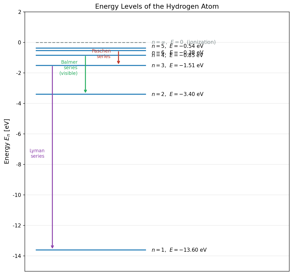
Fig. 1.13: Energy level diagram of the hydrogen atom. From \(n = 1\) (ground state) to \(n = \infty\) (ionization), energy is given by \(-13.6/n^2\) eV. Arrows represent electron transitions (light emission).
Derivation of the Rydberg Formula¶
🟡 Lina: Now let's derive the Rydberg formula. Using the frequency condition (Postulate 3), let's find the frequency of light emitted when an electron transitions from quantum number \(m\) to quantum number \(n\) (\(m > n\)).
When an electron falls from a higher energy level \(E_m\) to a lower energy level \(E_n\), since \(m > n\) we have \(1/m^2 < 1/n^2\). For example, with \(m = 3,\; n = 2\): \(E_3 = -13.6/9 \simeq -1.51\;\mathrm{eV}\), \(E_2 = -13.6/4 = -3.40\;\mathrm{eV}\). On the number line, \(-1.51\) is to the right of (greater than) \(-3.40\), so \(E_m > E_n\). In general, for negative numbers, the one with smaller absolute value is larger. Therefore
Since \(m > n\), we have \(1/n^2 - 1/m^2 > 0\), guaranteeing \(h\nu > 0\).
🔵 Kai: Great, we get positive energy. That flies out as a photon.
🟡 Lina: The relationship between light's frequency \(\nu\) and wavelength \(\lambda\) is \(c = \nu\lambda\) (\(c \simeq 3.0 \times 10^8\;\mathrm{m/s}\) is the speed of light). The wave oscillates \(\nu\) times per second, and each wavelength has length \(\lambda\), so the distance traveled in one second is \(\nu\lambda = c\). Using this:
Now let's express \(R_\infty\) in the Rydberg formula (1.6) in terms of fundamental constants. Our goal is to identify what \(R_\infty\) is in \(1/\lambda = R_\infty(1/n^2 - 1/m^2)\).
Dividing both sides of \(h\nu = 13.6\;\mathrm{eV}\,(1/n^2 - 1/m^2)\) by \(hc\) (since \(\nu/c = 1/\lambda\)):
So \(R_\infty = 13.6\;\mathrm{eV}/(hc)\). To write this in terms of fundamental constants, let's substitute \(a_0 = 4\pi\varepsilon_0\hbar^2/(m_e e^2)\) from equation (1.14) into the constant part \(e^2/(8\pi\varepsilon_0 a_0)\) of equation (1.15). Since \(1/a_0 = m_e e^2/(4\pi\varepsilon_0\hbar^2)\):
So \(13.6\;\mathrm{eV} = m_e e^4/(32\pi^2\varepsilon_0^2\hbar^2)\) (the \(32\pi^2\) comes from multiplying the denominator \(8\pi\varepsilon_0\) of \(e^2/(8\pi\varepsilon_0 a_0)\) with the denominator \(4\pi\varepsilon_0\hbar^2\) of \(1/a_0 = m_e e^2/(4\pi\varepsilon_0\hbar^2)\): \(8\pi \times 4\pi = 32\pi^2\)). Dividing by \(hc\):
Since \(\hbar = h/(2\pi)\), we have \(\hbar^2 = h^2/(4\pi^2)\). Substituting this, the numerator is \(m_e e^4\) (as found above), and looking at the denominator:
🔵 Kai: Um, substituting \(\hbar^2 = h^2/(4\pi^2)\) into the denominator, the \(\pi\)'s cancel between \(32\pi^2\) and \(4\pi^2\) giving \(32/4 = 8\), and \(h^2 \cdot h = h^3\), so it's \(8\varepsilon_0^2 h^3 c\). But earlier \(\hbar = h/(2\pi)\) appeared, yet here we write it in terms of \(h\). Is there a rule for when to use which?
🟡 Lina: Good observation. In this calculation, substituting \(\hbar^2 = h^2/(4\pi^2)\) made the \(\pi\)'s cancel cleanly, leaving an expression in \(h\) only. If instead you substituted \(h = 2\pi\hbar\) to rewrite in terms of \(\hbar\), the \(\pi\)'s would reappear and the formula would be slightly more complicated. As a general rule of thumb: pair \(h\) with frequency \(\nu\) (\(E = h\nu\)), and pair \(\hbar\) with angular frequency \(\omega\) (\(E = \hbar\omega\))—the \(2\pi\)'s cancel and things simplify. Angular frequency \(\omega\) is defined as \(\omega = 2\pi\nu\): while frequency \(\nu\) is "how many oscillations per second," \(\omega\) is "how many radians (angle) per second." One oscillation covers \(2\pi\) radians (\(360°\)), so \(\omega = 2\pi\nu\). We'll use it extensively from the next chapter onward, so for now just remember the guideline for when to use \(h\) vs. \(\hbar\).
⚪ Mei: So the practical policy is "choose whichever makes the \(\pi\)'s disappear."
🟡 Lina: Historically, the Rydberg constant is standardly written in terms of \(h\), so let's continue as is. Substituting the actual values \(m_e = 9.109 \times 10^{-31}\;\mathrm{kg}\), \(e = 1.602 \times 10^{-19}\;\mathrm{C}\), \(\varepsilon_0 = 8.854 \times 10^{-12}\;\mathrm{F/m}\), \(h = 6.626 \times 10^{-34}\;\mathrm{J \cdot s}\), \(c = 2.998 \times 10^8\;\mathrm{m/s}\) gives \(R_\infty \simeq 1.097 \times 10^7\;\mathrm{m^{-1}}\), in perfect agreement with the experimental value. In summary:
Using this:
🔵 Kai: This is exactly the Rydberg formula (1.6) from before! For 30 years nobody knew "why this formula holds," and it comes out from just Bohr's three postulates...
🟡 Lina: Yes! Bohr's model theoretically derived the Rydberg formula that had been a mystery for 30 years. Moreover, it calculated the Rydberg constant from fundamental constants alone (\(m_e\), \(e\), \(\varepsilon_0\), \(h\), \(c\)), achieving perfect agreement with experiment. In Fig. 1.14 "Wavelength distribution of the hydrogen atom spectral series (logarithmic axis)", I've summarized which wavelength regions each series appears in.
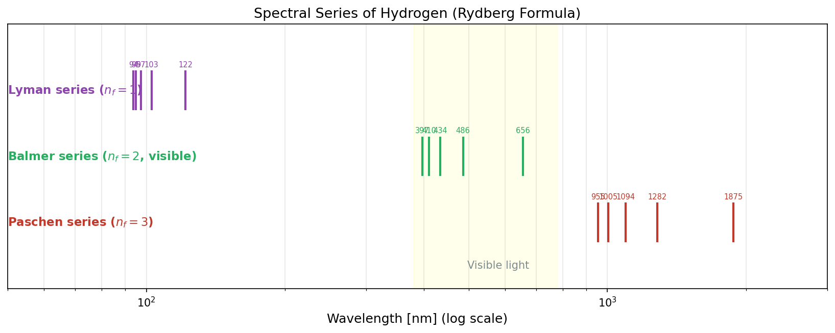
Fig. 1.14: Wavelength distribution of the hydrogen atom spectral series (logarithmic axis). The Lyman series (falling to \(n_f = 1\)) is in the ultraviolet, the Balmer series (falling to \(n_f = 2\)) is in visible light (yellow band), and the Paschen series (falling to \(n_f = 3\)) is in the infrared. The starting point of each series corresponds to the ionization energy, and lines become more densely packed at higher \(n_i\).
🟡 Lina: Let me organize what we've achieved so far. What Bohr's model solved: - Atomic stability: Electrons don't radiate electromagnetic waves when in stationary states (Postulate 1) - Discreteness of spectra: Since allowed orbits are discrete, energy differences are discrete, and the frequencies of emitted light are discrete - Derivation of the Rydberg formula: Completely reproduced from \(E_n = -13.6\;\mathrm{eV}/n^2\) and the frequency condition
⚪ Mei: It beautifully addresses all three crises.
Limitations of the Bohr Model¶
🟡 Lina: However, I must also mention that Bohr's model has limitations.
🔵 Kai: Limitations? Even though it derived the Rydberg formula so beautifully...
🟡 Lina: Bohr's model brilliantly explained the spectrum of the hydrogen atom (1 electron), but it couldn't be applied to atoms with 2 or more electrons (helium and beyond). Also, "why doesn't it radiate in stationary states?" and "why is angular momentum an integer multiple of \(\hbar\)?"—it couldn't answer these "whys." Let me organize this (Table 1.4 "Successes and limitations of the Bohr model").
Table 1.4: Successes and limitations of the Bohr model
| Successes | Limitations/Unresolved issues |
|---|---|
| Completely reproduces hydrogen atom spectrum | Cannot be applied to multi-electron atoms (helium and beyond) |
| Derives Rydberg constant from fundamental constants | No explanation for "why no radiation in stationary states" |
| Explains atomic stability | No basis for "why \(L = n\hbar\)" |
| Predicts correct order of magnitude for atomic size | Cannot predict spectral line intensities (brightness) |
🔵 Kai: "Why integer multiples of \(\hbar\)?"—come to think of it, Bohr just said "assume this" without explaining the reason. Just because an assumption gives correct results doesn't necessarily mean the assumption itself is correct...?
🟡 Lina: Exactly. This is the idea from the Prologue that "physics models are merely the best hypotheses that don't contradict experiment." Bohr's model doesn't contradict hydrogen atom experiments, but a deeper theory is needed to explain "why it's so"—that's why it's called a "provisional model."
⚪ Mei: It gives the right answer but with unclear justification—the true "why" requires a deeper theory.
🟡 Lina: That's right. The true answer—the answer to "why"—was first provided by the quantum mechanics completed by Heisenberg and Schrödinger in 1925-26. Bohr's model played an historically crucial role as a bridge from classical physics to quantum mechanics.
🔵 Kai: Classical → Bohr → full quantum mechanics—that's the flow.
🟡 Lina: Yes. And in this journey, to answer the "why" of the Bohr model, from Ch. 4 onward we'll build quantum mechanics step by step from the concept of probability amplitudes.
✅ Comprehension Check: List two main limitations of the Bohr model.
Answer
① It cannot explain the spectra of atoms with two or more electrons (helium and beyond). ② It cannot explain the fundamental reasons for "why no electromagnetic radiation in stationary states" or "why angular momentum is an integer multiple of \(\hbar\)" (these were only postulated, not derived).
✅ Comprehension Check: When Bohr's quantum condition \(L = n\hbar\) is applied to the hydrogen atom, how many times larger is the orbital radius for \(n = 2\) compared to \(n = 1\)?
Answer
From equation (1.13), \(r_n \propto n^2\), so \(r_2 / r_1 = 2^2 / 1^2 = 4\) times larger.
✅ Comprehension Check: Using the Rydberg formula, calculate the wavelength of light emitted when the electron in a hydrogen atom transitions from \(n = 3\) to \(n = 2\).
Answer
\(\displaystyle \frac{1}{\lambda} = R_\infty\left(\frac{1}{2^2} - \frac{1}{3^2}\right) = 1.097 \times 10^7 \left(\frac{1}{4} - \frac{1}{9}\right) = 1.097 \times 10^7 \times \frac{5}{36} \simeq 1.524 \times 10^6\;\mathrm{m^{-1}}\)
\(\lambda \simeq 6.56 \times 10^{-7}\;\mathrm{m} = 656\;\mathrm{nm}\) (red light—the \(H_\alpha\) line of the Balmer series).
📝 Exercises:
- Calculation of the hydrogen atom ionization energy using the Bohr model → Problem M-1. Derivation of Hydrogen Atom Energy Levels Using the Bohr Model
Summary — The Limits of Classical Physics and the Dawn of Quantum Theory¶
🟡 Lina: Let's organize what we've seen in this chapter (Table 1.5 "Three crises of classical physics and their quantum resolutions"). At the end of the 19th century, classical physics faced three serious crises.
Table 1.5: Three crises of classical physics and their quantum resolutions
| Crisis | Core of the problem | Solver and year | Key idea |
|---|---|---|---|
| Ultraviolet catastrophe of black-body radiation | Radiated energy diverges to infinity at high frequencies | Planck (1900) | Energy comes in integer multiples of \(h\nu\) (quantum hypothesis) |
| Mystery of the photoelectric effect | Color of light is decisive, intensity is irrelevant | Einstein (1905) | Light is a particle (photon) with energy \(h\nu\) |
| Atomic stability | Electron spirals in and collapses in \(\sim 10^{-11}\) s | Bohr (1913) | Only discrete orbits are allowed for electrons |
🟡 Lina: Looking at these three breakthroughs chronologically, you can see that the foundations of quantum theory were laid in just 13 years. Take a look at Fig. 1.15 "Timeline of the birth of quantum theory".
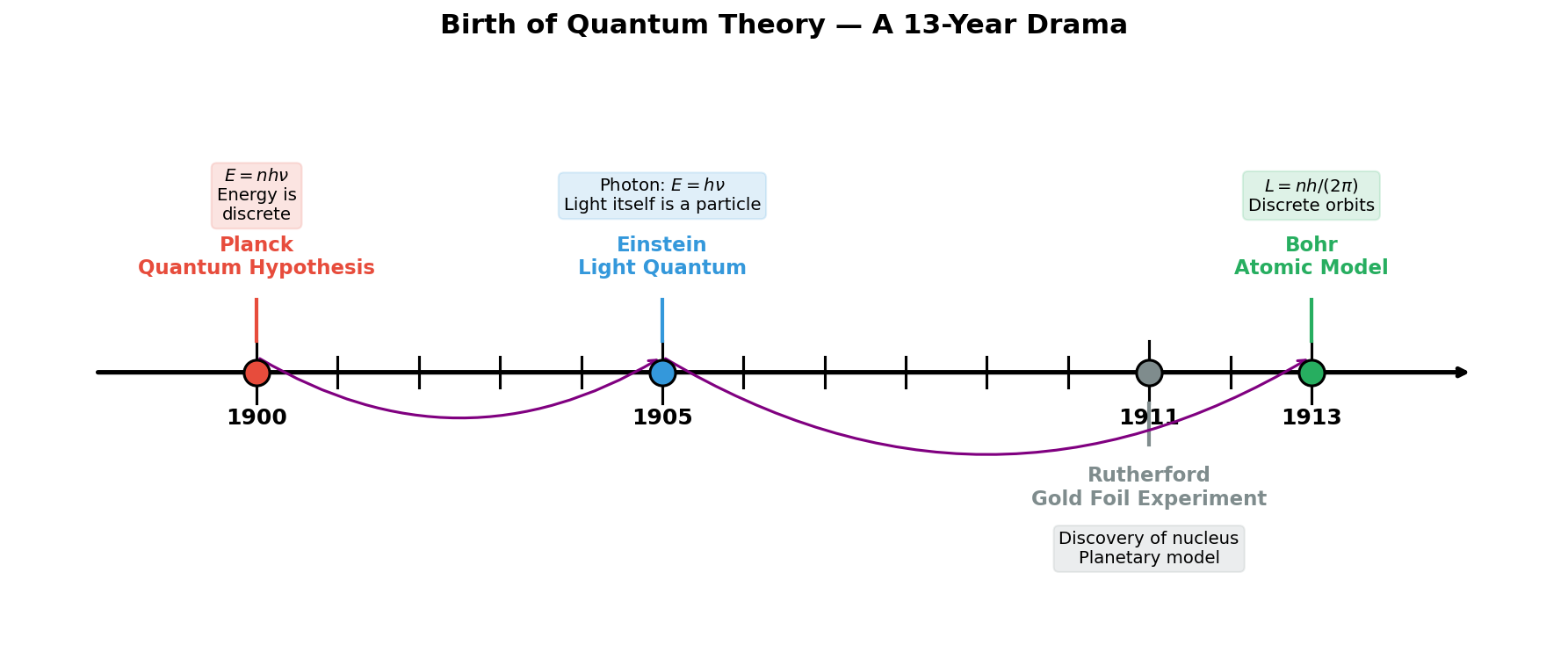
Fig. 1.15: Timeline of the birth of quantum theory. Planck's quantum hypothesis (1900) → Einstein's light quantum hypothesis (1905) → Rutherford's discovery of the nucleus (1911) → Bohr's atomic model (1913). Each discovery builds on the previous achievement, showing how quantum ideas were inherited and developed.
🔵 Kai: What they all have in common is "discreteness." Energy is discrete, light comes in chunks, orbits are discrete... But "why is nature discrete?"—that reason hasn't appeared yet, has it?
🟡 Lina: Good catch. Actually, answering that "why" is the substance of the quantum mechanics we're about to learn. Both Planck and Bohr only showed "if we assume discreteness, the results match experiment," without explaining the underlying reason. The justification will become visible from Ch. 4 onward, when we study wave functions and boundary conditions. For now, firmly grasp the starting point that "discreteness is an experimental fact."
⚪ Mei: So the three crises of this chapter only demonstrated "assuming discreteness solves the problem," while "why discrete" remains unresolved and is carried forward to the following chapters.
🟡 Lina: From "continuous" to "discrete"—this is the most fundamental paradigm shift from classical physics to quantum theory. And the constant that runs through all of this is
Planck's constant \(h\). The fact that this constant has a finite, non-zero value is what makes the world "discrete."
🔵 Kai: So what would happen if \(h\) were zero? It wouldn't be discrete anymore?
🟡 Lina: Exactly. If \(h = 0\), all quantum effects vanish and we return to classical physics. And \(h\) is very small but not zero—so at everyday scales classical physics is a good approximation, while at the atomic scale quantum effects dominate. You could rephrase it as "classical physics is the \(h \to 0\) limit."
⚪ Mei: So the smallness of \(h\) determines "the boundary between classical and quantum."
🔵 Kai: I see... Because \(h\) isn't zero the world is discrete, but because it's small we normally don't notice. Also, it was impressive that Einstein is one of the founders of quantum theory. He said "light is a particle" himself, and then later criticized quantum mechanics... What bothered him so much?
🟡 Lina: Good question. The 1905 light quantum hypothesis, the 1917 theory of stimulated emission—Einstein was on the side that created quantum theory. But when quantum mechanics was completed, he felt deep discomfort with the interpretation that "nature's behavior is fundamentally probabilistic." The famous phrase "God does not play dice" was his expression of that discomfort. We'll examine in detail what the problem was in Ch. 21 (quantification of stimulated emission) and Ch. 23 (the EPR argument and Bell's inequality). Look forward to it.
Preview of the Next Chapter¶
🟡 Lina: In this chapter, we've seen the three crises of classical physics and the "discreteness" solutions to each. But a major mystery still remains.
Einstein said "light is also a particle (photon)." But light being a wave was established fact through interference experiments. Being a wave and a particle at the same time—what does this even mean?
Furthermore, in 1924—about 10 years after Bohr's model—de Broglie made the reverse proposal. "If light is also a particle, might particles like electrons also be waves?"—and this was experimentally confirmed. Look at Fig. 1.16 "Formation of electron double-slit interference pattern". When electrons are fired one at a time through slits, at first only random dots appear, but as the number increases, a wave interference pattern emerges. This experiment is the clearest evidence that de Broglie's "matter wave" idea is correct, and it becomes the starting point for the next chapter.
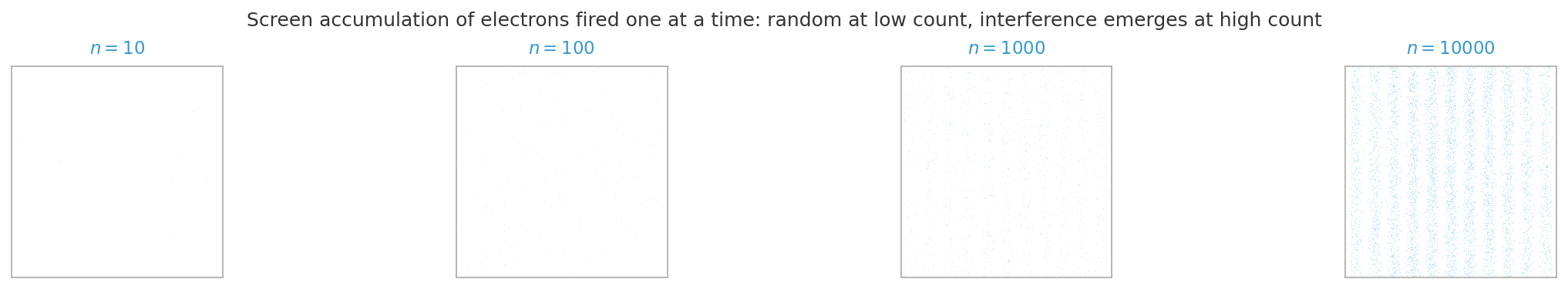
Fig. 1.16: Formation of electron double-slit interference pattern. Time evolution of the impact distribution when electrons are fired one at a time through a double slit. With few electrons, only random spots appear, but as many accumulate, a wave interference pattern emerges. This experiment clearly demonstrates that "particles possess wave properties" and serves as the starting point for de Broglie's matter waves, covered in the next chapter.
In the next chapter, we'll follow this bold hypothesis and the electron diffraction experiment that dramatically confirmed it. Let's witness the moment when the boundary between particle and wave dissolves.
Practice Problems¶
📝 Exercises:
- Calculation to appreciate the smallness of Planck's constant → Problem B-1. Appreciating the Smallness of Planck's Constant
- Calculating work function and threshold frequency → Problem B-2. Work Function and Threshold Frequency
- Order-of-magnitude estimate of classical atomic collapse time → Problem M-3. Order-of-magnitude estimate of classical atomic collapse time
- Calculation of the hydrogen atom ionization energy using the Bohr model → Problem M-1. Derivation of Hydrogen Atom Energy Levels Using the Bohr Model
References¶
- M. Planck, "Zur Theorie des Gesetzes der Energieverteilung im Normalspectrum," Verhandlungen der Deutschen Physikalischen Gesellschaft 2, 237–245 (1900).
- A. Einstein, "Über einen die Erzeugung und Verwandlung des Lichtes betreffenden heuristischen Gesichtspunkt," Annalen der Physik 17, 132–148 (1905).
- N. Bohr, "On the Constitution of Atoms and Molecules," Philosophical Magazine 26, 1–25 (1913).
- R. P. Feynman, R. B. Leighton, M. Sands, The Feynman Lectures on Physics, Vol. III (Addison-Wesley, 1965), Ch. 1.
- C. Rovelli, Reality Is Not What It Seems (Penguin, 2016), Ch. 6.
- 清水明『新版 量子論の基礎——その本質のやさしい理解のために』(サイエンス社, 2004), 第 1 章「古典物理学の破綻」.
- D. J. Griffiths, Introduction to Quantum Mechanics, 3rd ed. (Cambridge University Press, 2018), §1.1.
Feedback on this page
Let us know if something was unclear, incorrect, or could be improved.