Appendix G: Derivation of the Einstein Equations
Story so far: In Ch. 6, we presented the Einstein equation \(G_{\mu\nu} = 8\pi G\, T_{\mu\nu}\) as "spacetime curvature = matter energy" without derivation. But where does this equation come from? Just as Newton's mechanics can derive \(F = ma\) from \(L = T - V\), the Einstein equations can also be derived from an action principle.
Goals of this appendix
- Follow the variation of the Einstein-Hilbert action line by line to completely derive the Einstein equations
- As a practical example of the variational method, this also serves as a bridge to the Polyakov action in string theory (Ch. 13)
G.1: Motivation — Why Derive from an Action Principle
🟡 Lina: Looking back at the history of physics, fundamental equations have always been obtained through two routes.
Table G.1: Comparison of derivation routes for fundamental equations
| Field | Direct reasoning | Action principle |
|---|---|---|
| Mechanics | Newton's equation of motion \(F = ma\) | Variation of Lagrangian \(L = T - V\) |
| Electromagnetism | Maxwell's equations | Electromagnetic field action \(S = -\frac{1}{4}\int F_{\mu\nu}F^{\mu\nu}\sqrt{-g}\,d^4x\) |
| General relativity | Einstein's physical reasoning (1915) | Variation of Einstein-Hilbert action |
🔵 Kai: In Newton's case, \(F = ma\) came first, and later it could be re-derived from the Lagrangian. Is it the same for the Einstein equations?
🟡 Lina: Yes. Einstein arrived at the equations through the equivalence principle, general covariance, and consistency with the Newtonian limit. Almost simultaneously, Hilbert was working on a formulation using the action principle. Historically, "the equation came first, the action came after." But the action principle has decisive advantages.
🔵 Kai: What advantages?
🟡 Lina: There are three:
- Symmetries are automatically guaranteed — If the action is a scalar, the equations derived from it are automatically covariant under general coordinate transformations
- Unified framework — Both gravity and matter go into the same action \(S = S_{EH} + S_M\), and everything comes from \(\delta S = 0\)
- Path to quantization — As we saw in field theory (Quantum Field Theory Chapters 10–11), this becomes the starting point for the path integral \(\int \mathcal{D}[g]\,e^{iS/\hbar}\)
🔵 Kai: Is string theory the same spirit?
🟡 Lina: Exactly. The Polyakov action in Ch. 13 also has the same structure of "varying a scalar action on the worldsheet." So mastering the variational technique here will make the string theory derivation much smoother to read.
For the basics of variational calculus, see General Relativity General Relativity Appendix C; for variation of field Lagrangians, see Quantum Field Theory Quantum Field Theory Ch. 3.
G.2: The Einstein-Hilbert Action
G.2.1: Requirements That Determine the Form of the Action
🟡 Lina: To determine the gravitational action \(S_{EH}\), we impose the following requirements:
- General coordinate invariance — The action is a scalar (its value doesn't change under coordinate transformations)
- Constructed only from the metric tensor \(g_{\mu\nu}\) and its derivatives — The degrees of freedom of gravity are in the metric
- Equations of motion are second order — We want solutions to be determined by specifying initial position and velocity. In general, if the Lagrangian contains \(n\)-th order derivatives of the variable, the Euler-Lagrange equation becomes a \(2n\)-th order differential equation (because integration by parts is performed \(n\) times during variation). Since \(R\) contains second derivatives of the metric, one might naively expect the equations of motion to be fourth order. However, thanks to the special structure of \(R\), the terms containing \(\delta R_{\mu\nu}\) become a total derivative (boundary term) and drop out, resulting in second-order equations (we'll confirm this in G.3.3)
- Simplest possible — The lowest-order terms possible
🔵 Kai: What scalars specifically satisfy all those conditions?
🟡 Lina: The Ricci scalar \(R\) that we learned about in General Relativity General Relativity Ch. 13 is exactly that. \(R = g^{\mu\nu}R_{\mu\nu}\) is the simplest scalar containing second derivatives of the metric. Combining it with the volume element \(\sqrt{-g}\,d^4x\) in 4 dimensions:
Here we use natural units \(c = 1\) (restoring \(c\) gives \(1/(16\pi G) \to c^4/(16\pi G)\)).
🔵 Kai: Why is \(\sqrt{-g}\) necessary?
🟡 Lina: With \(d^4x\) alone, a Jacobian appears under coordinate transformations. \(\sqrt{-g}\,d^4x\) is the generally coordinate-invariant volume element. We learned this in General Relativity General Relativity Ch. 7.
⚪ Mei: So \(\sqrt{-g}\) is a correction factor to "measure volume correctly regardless of the choice of coordinates."
✅ Comprehension Check: What are the four requirements that determine the form of the Einstein-Hilbert action?
Answer
(1) General coordinate invariance (action is a scalar), (2) constructed only from the metric tensor and its derivatives, (3) up to second-order derivatives (equations of motion are second order), (4) simplest possible (lowest-order terms possible).
G.2.2: Adding the Cosmological Constant Term
🟡 Lina: There's another term that satisfies the requirements. A volume multiplied by the constant \(\Lambda\) (cosmological constant):
This is also a generally coordinate-invariant scalar, constructed from zeroth-order derivatives of the metric (no derivatives). Since it's the simplest possible term, there's no reason in principle to exclude it.
✅ Comprehension Check: Why is the cosmological constant term \(S_\Lambda\) allowed in the gravitational action?
Answer
The cosmological constant term is a generally coordinate-invariant scalar constructed from zeroth-order derivatives of the metric (containing no derivatives), making it the simplest possible term that satisfies the symmetry requirements, so there is no reason in principle to exclude it.
🟡 Lina: Combining this with the earlier \(S_{EH}\), the total gravitational action is:
The \(-2\Lambda\) coefficient is a convention, chosen so that \(\Lambda g_{\mu\nu}\) appears in the final Einstein equations.
⚪ Mei: So we've combined the \(R\) term and the constant term into a single integral.
G.2.3: The Total Action
Denoting the matter field action as \(S_M\), the total action is:
The principle of least action:
This gives the Einstein equations. Below, we carry out this variation.
✅ Comprehension Check: What is the scalar quantity contained in the integrand of the Einstein-Hilbert action?
Answer
The scalar curvature \(R\) (and the cosmological constant \(\Lambda\)).
✅ Comprehension Check: In the principle of least action, what do we vary the total action \(S\) with respect to, and set to zero?
Answer
We vary with respect to the metric tensor \(g^{\mu\nu}\) and set it to zero.
G.3: Carrying Out the Variation — Three Contributions
🟡 Lina: Since \(R = g^{\mu\nu}R_{\mu\nu}\), the variation of the integrand \(\sqrt{-g}\,R = \sqrt{-g}\,g^{\mu\nu}R_{\mu\nu}\) splits into three parts by the product rule:
We'll call these the first term, second term, and third term respectively. The overall structure is shown in Fig. G.1 "Decomposition of the variation of the Einstein–Hilbert action".
🔵 Kai: Since it's a product of three factors, the differentiation rule splits it into three parts.
🟡 Lina: Right. The diagram shows them in numerical order, but we'll proceed in order of computational difficulty: first the technically independent third term (calculating \(\delta\sqrt{-g}\)), then the trivial first term (which stays as is), and finally the crucial second term (Palatini's identity).
%%{init: {"theme": "default", "themeCSS": ".edgePath .path, .flowchart-link { stroke-width: 2px !important; }"}}%%
flowchart TD
    A["δ(√-g · g^μν R_μν)"] --> B["Term 1<br>√-g R_μν δg^μν"]
    A --> C["Term 2<br>√-g g^μν δR_μν"]
    A --> D["Term 3<br>R · δ√-g"]
    B --> E["Stays as is<br>→ R_μν δg^μν"]
    C --> F["Palatini's identity<br>∇_α V^α (total derivative)"]
    F --> G["Boundary term → 0"]
    D --> H["Formula for δ√-g<br>→ -½ R g_μν δg^μν"]
    E --> I["Combined: (R_μν - ½ g_μν R) δg^μν"]
    H --> I
Fig. G.1: Decomposition of the variation of the Einstein–Hilbert action
G.3.1: Third Term: Calculating \(\delta\sqrt{-g}\)
🟡 Lina: Let's first deal with the most technically independent third term. Writing \(g \equiv \det(g_{\mu\nu})\), we want to find the variation of \(\sqrt{-g}\).
Step 1: Variation of the determinant (Jacobi's formula)
For the determinant of a matrix \(A\), in general:
This was derived in General Relativity General Relativity Appendix C. Applying it to the metric tensor:
🔵 Kai: \(\delta g_{\mu\nu}\) and \(\delta g^{\mu\nu}\) are different things, right? What's the relationship?
🟡 Lina: Good question. Varying both sides of \(g^{\mu\alpha}g_{\alpha\nu} = \delta^\mu_\nu\):
Multiplying both sides by \(g^{\nu\beta}\) and rearranging:
Therefore:
⚪ Mei: The sign flips when raising and lowering indices. Same structure as differentiating an inverse matrix.
🟡 Lina: That's right.
Step 2: Writing \(\delta g\) in terms of \(\delta g^{\mu\nu}\)
Using the relation above:
Step 3: Finding \(\delta\sqrt{-g}\)
The variation of \(\sqrt{-g}\) by the chain rule:
Substituting \(\delta g = -g\,g_{\mu\nu}\,\delta g^{\mu\nu}\):
Since \(g < 0\), we have \(-g > 0\), and \(\sqrt{-g}\) is well-defined as a real number. From the definition of \(\sqrt{-g}\), \((\sqrt{-g})^2 = -g\), so we can write \(g = -(\sqrt{-g})^2\). Substituting this into the numerator:
The last equality is simply canceling one factor of \(\sqrt{-g}\) between numerator and denominator.
Therefore:
⚪ Mei: What a clean form! \(g_{\mu\nu}\,\delta g^{\mu\nu}\) is a contraction of indices, so it's a scalar.
🟡 Lina: Right. So the third term is:
📝 Exercises:
- Derivation of \(\delta\sqrt{-g}\) → Problem M-1. Derivation of \(\delta\sqrt{-g}\)
G.3.2: First Term: \(\sqrt{-g}\,R_{\mu\nu}\,\delta g^{\mu\nu}\)
🟡 Lina: The first term stays as is:
Nothing needs to be computed. \(R_{\mu\nu}\) behaves like a "constant" with respect to the variation of \(g^{\mu\nu}\).
G.3.3: Second Term: \(\sqrt{-g}\,g^{\mu\nu}\,\delta R_{\mu\nu}\) — Palatini's Identity
🟡 Lina: Here is the heart of the derivation. Since the Ricci tensor \(R_{\mu\nu}\) is written in terms of derivatives of the Christoffel symbols \(\Gamma^\alpha_{\mu\nu}\), changing \(g^{\mu\nu}\) changes \(\Gamma\), which in turn changes \(R_{\mu\nu}\).
Step 1: \(\delta\Gamma^\alpha_{\mu\nu}\) is a tensor
🔵 Kai: \(\Gamma^\alpha_{\mu\nu}\) itself isn't a tensor, but its variation is a tensor?
🟡 Lina: Yes. Recall that the coordinate transformation law for \(\Gamma\) has an extra term involving "second derivatives of the coordinate transformation"—that is, when performing a coordinate change \(x \to x'\), terms like \(\partial^2 x^\mu / \partial x'^\alpha \partial x'^\beta\) appear (see General Relativity General Relativity Ch. 7). "Transforming as a tensor" means that under a coordinate change, each component changes according to a regular rule (multiplying by one transformation matrix per index). \(\Gamma\) has extra terms that deviate from this rule, so it "is not a tensor."
However, these extra terms are determined solely by the choice of coordinate system and do not depend on the value of the metric. Specifically, the coordinate transformation law for \(\Gamma\) has the structure "part that transforms tensorially + extra term proportional to second derivatives of the coordinate transformation \(\partial^2 x/\partial x'^2\)." This extra term is determined by the coordinate transformation alone and does not depend at all on what value \(g_{\mu\nu}\) takes. So while \(\Gamma\) itself is not a tensor, when we slightly change the metric \(g_{\mu\nu} \to g_{\mu\nu} + \delta g_{\mu\nu}\) in the same coordinate system, and consider the difference \(\delta\Gamma = \Gamma[g + \delta g] - \Gamma[g]\) between the pre-variation connection \(\Gamma[g]\) and the post-variation connection \(\Gamma[g + \delta g]\), the extra terms appear in exactly the same form in both and cancel.
🔵 Kai: Ah, I see. The extra terms are determined only by "the choice of coordinate system," so they don't change when you change the metric. So they cancel when you take the difference—just like common terms canceling in subtraction.
🟡 Lina: Exactly. As a result, \(\delta\Gamma^\alpha_{\mu\nu}\) transforms as a tensor.
Step 2: Definition and variation of the Ricci tensor
The Ricci tensor is a contraction of the Riemann tensor (see General Relativity General Relativity Ch. 13):
We compute the variation of this. "Variation" means finding the change when we slightly modify the metric \(g_{\mu\nu} \to g_{\mu\nu} + \delta g_{\mu\nu}\), which causes \(\Gamma \to \Gamma + \delta\Gamma\). Since \(\delta\Gamma\) is infinitesimal, we ignore terms of second order and higher in \(\delta\Gamma\) (like \((\delta\Gamma)^2\)) and keep only first-order terms—this is the same operation as keeping only the first-order term in a Taylor expansion. The partial derivative terms \(\partial_\alpha\Gamma^\alpha_{\mu\nu}\) are linear (first-order) in \(\Gamma\), so they simply become \(\partial_\alpha(\delta\Gamma^\alpha_{\mu\nu})\). For the \(\Gamma\Gamma\) terms, we apply the product rule (\((fg)' = f'g + fg'\)). For example, the variation of \(\Gamma^\alpha_{\alpha\beta}\Gamma^\beta_{\mu\nu}\) gives two terms: \(\delta(\Gamma^\alpha_{\alpha\beta})\cdot\Gamma^\beta_{\mu\nu} + \Gamma^\alpha_{\alpha\beta}\cdot\delta(\Gamma^\beta_{\mu\nu})\). Similarly, the variation of \(-\Gamma^\alpha_{\nu\beta}\Gamma^\beta_{\mu\alpha}\) gives \(-\delta(\Gamma^\alpha_{\nu\beta})\cdot\Gamma^\beta_{\mu\alpha} - \Gamma^\alpha_{\nu\beta}\cdot\delta(\Gamma^\beta_{\mu\alpha})\). Combining everything:
⚪ Mei: This is incredibly complicated...
🟡 Lina: Actually, since \(\delta\Gamma\) is a tensor, we can replace the partial derivatives \(\partial_\alpha\) with covariant derivatives \(\nabla_\alpha\). Let's verify this explicitly. Expanding \(\nabla_\alpha(\delta\Gamma^\rho_{\mu\nu})\) using the definition of the covariant derivative (see General Relativity General Relativity Ch. 7):
Similarly, expanding \(\nabla_\nu(\delta\Gamma^\rho_{\mu\alpha})\):
🔵 Kai: I'm just applying the definition of the covariant derivative, but there are so many terms... Does this really match the messy expression above?
🟡 Lina: It does. Taking the difference \(\nabla_\alpha(\delta\Gamma^\rho_{\mu\nu}) - \nabla_\nu(\delta\Gamma^\rho_{\mu\alpha})\), and then contracting by setting \(\rho = \alpha\) (here \(\rho\) was a free index up to now, but we make it the same letter as \(\alpha\) and sum), the partial derivative terms give \(\partial_\alpha(\delta\Gamma^\alpha_{\mu\nu}) - \partial_\nu(\delta\Gamma^\alpha_{\mu\alpha})\). Let's look at the remaining \(\Gamma \cdot \delta\Gamma\) terms explicitly.
Expanding \(\nabla_\alpha(\delta\Gamma^\alpha_{\mu\nu})\) by the definition of the covariant derivative (after performing the contraction \(\rho = \alpha\)), in addition to the partial derivative \(\partial_\alpha(\delta\Gamma^\alpha_{\mu\nu})\), three \(\Gamma\cdot\delta\Gamma\) terms appear:
Similarly, expanding \(\nabla_\nu(\delta\Gamma^\alpha_{\mu\alpha})\):
Taking the difference, a total of 6 \(\Gamma\cdot\delta\Gamma\) terms appear. Among these, the 4th term of the first equation \(-\Gamma^\sigma_{\alpha\nu}(\delta\Gamma^\alpha_{\mu\sigma})\) and the 4th term of the second equation \(+\Gamma^\sigma_{\nu\alpha}(\delta\Gamma^\alpha_{\mu\sigma})\) cancel exactly due to the symmetry of \(\Gamma\) in its lower indices \(\Gamma^\sigma_{\alpha\nu} = \Gamma^\sigma_{\nu\alpha}\). Writing out the remaining 4 terms:
- 2nd term of the first equation: \(+\Gamma^\alpha_{\alpha\sigma}(\delta\Gamma^\sigma_{\mu\nu})\)
- 3rd term of the first equation: \(-\Gamma^\sigma_{\alpha\mu}(\delta\Gamma^\alpha_{\sigma\nu})\)
- 2nd term of the second equation: \(-\Gamma^\alpha_{\nu\sigma}(\delta\Gamma^\sigma_{\mu\alpha})\)
- 3rd term of the second equation: \(+\Gamma^\sigma_{\nu\mu}(\delta\Gamma^\alpha_{\sigma\alpha})\)
That these match the 4 \(\Gamma\cdot\delta\Gamma\) terms in \(\delta R_{\mu\nu}\) at the beginning of Step 2 can be verified by renaming dummy indices (for example, in the 3rd term of the second equation \(+\Gamma^\sigma_{\nu\mu}(\delta\Gamma^\alpha_{\sigma\alpha})\), substituting \(\sigma \to \beta\) gives \(+\Gamma^\beta_{\nu\mu}(\delta\Gamma^\alpha_{\beta\alpha})\), and using the symmetry of \(\Gamma\) in its lower indices \(\Gamma^\beta_{\nu\mu} = \Gamma^\beta_{\mu\nu}\) gives \(+\Gamma^\beta_{\mu\nu}(\delta\Gamma^\alpha_{\beta\alpha})\). This corresponds to the term \((\delta\Gamma^\alpha_{\alpha\beta})\Gamma^\beta_{\mu\nu}\) in the original expression, differing only in the order of factors). The remaining terms can be similarly verified through dummy index renaming (readers who want to trace the correspondence of all 4 terms one by one should refer to the exercises in General Relativity General Relativity Appendix C). The key point is that the connection coefficient terms contained in the definition of the covariant derivative absorb the 4 \(\Gamma\cdot\delta\Gamma\) terms of \(\delta R_{\mu\nu}\) exactly, with nothing left over. This is not a coincidence but a direct consequence of \(\delta\Gamma\) being a tensor—since the covariant derivative is the partial derivative of a tensor plus connection coefficient corrections, any expression containing partial derivatives of the tensor \(\delta\Gamma\) necessarily organizes into the covariant derivative form. The result is:
Note that the direction of differentiation (\(\alpha\) and \(\nu\)) differs between the first and second terms.
This is the Palatini identity.
🔵 Kai: The partial derivatives and the \(\Gamma\) product terms all get absorbed into the covariant derivatives.
⚪ Mei: Of the 6 terms, 2 cancel and the remaining 4 match perfectly—beautiful structure.
🔵 Kai: I understand that they get absorbed into the covariant derivatives, but what happens in the next Step 3 when we multiply by \(g^{\mu\nu}\)?
🟡 Lina: Good question. Since the covariant derivative of a tensor is a tensor, this equation is coordinate-independent. Next, let's multiply by \(g^{\mu\nu}\) and organize it into a total derivative form.
Step 3: Making \(g^{\mu\nu}\,\delta R_{\mu\nu}\) into a total derivative
Multiplying by \(g^{\mu\nu}\):
For the Levi-Civita connection, the metric compatibility condition \(\nabla_\alpha g^{\mu\nu} = 0\) (see General Relativity General Relativity Ch. 12) holds, so we can bring \(g^{\mu\nu}\) inside the covariant derivative. First, for the first term:
Next, for the second term:
⚪ Mei: Thanks to the metric compatibility condition, \(g^{\mu\nu}\) can be brought inside the derivative.
🔵 Kai: But the first term is \(\nabla_\alpha(\cdots)\) and the second term is \(\nabla_\nu(\cdots)\)—the derivative indices are different. How do we combine them?
🟡 Lina: Good observation. As they stand, we can't combine them into a single divergence. Here \(\alpha\) in the first term and \(\nu\) in the second term are both dummy indices (the same letter appears twice and is contracted). What we ultimately want to do is write both terms in the same form \(\nabla_\lambda(\text{something})\) and combine them as \(\nabla_\lambda(\text{first term's content} - \text{second term's content})\). To do this, we need to make the derivative indices the same letter \(\lambda\).
🔵 Kai: Dummy indices don't change the value when you rename them, right? Like \(\sum_i a_i = \sum_j a_j\).
🟡 Lina: Exactly. For example, in 2 dimensions, whether you write \(\sum_{\nu=0}^{1} A_\nu B^\nu = A_0 B^0 + A_1 B^1\) or \(\sum_{\alpha=0}^{1} A_\alpha B^\alpha = A_0 B^0 + A_1 B^1\), it's the same value—the letter is just a label for "the number being summed over."
So let me explain what we'll do in two steps:
Step A: Rename the dummy indices in the second term \(\nabla_\nu(g^{\mu\nu}\,\delta\Gamma^\alpha_{\mu\alpha})\). The goal is to align the derivative index to \(\lambda\). We want to change \(\nu \to \lambda\). Let's check that there's no problem leaving \(\alpha\) as is—\(\nabla_\lambda(g^{\mu\lambda}\,\delta\Gamma^\alpha_{\mu\alpha})\) has \(\lambda\) appearing once up and once down, and \(\alpha\) appearing once up and once down, so no violation of the contraction rules. OK.
🔵 Kai: Wait. What if I changed \(\nu \to \alpha\)?
🟡 Lina: That would give \(\nabla_\alpha(g^{\mu\alpha}\,\delta\Gamma^\alpha_{\mu\alpha})\), where \(\alpha\) appears in 3 places. This violates Einstein's summation convention—the same index should appear as an up-down pair only once for summation. So \(\nu\) must be changed to a new letter different from \(\alpha\).
Step B: Look at the first term \(\nabla_\alpha(g^{\mu\nu}\,\delta\Gamma^\alpha_{\mu\nu})\). Here \(\alpha\) is both the derivative index and the upper index of \(\Gamma\) (it appears in both places and is contracted). Renaming this \(\alpha\) to \(\lambda\) gives \(\nabla_\lambda(g^{\mu\nu}\,\delta\Gamma^\lambda_{\mu\nu})\).
Now both terms are in the form \(\nabla_\lambda(\cdots)\), so we can subtract the contents of the parentheses and combine them into one.
🔵 Kai: Is it okay to use \(\lambda\) in both terms? Won't they get mixed up?
🟡 Lina: It's fine. The point is that ultimately we're combining the two terms into a single covariant derivative \(\nabla_\lambda(\text{first term's content} - \text{second term's content})\). After combining, \(\lambda\) becomes one dummy index throughout the whole expression. For example, it's the same operation as combining \(\sum_i a_i - \sum_j b_j\) into \(\sum_i(a_i - b_i)\) in ordinary addition—you rename \(j\) to \(i\) and then subtract. As long as dummy indices don't overlap within each term, there's no problem.
⚪ Mei: So since the value doesn't change when you rename, we unified the derivative indices of both terms to \(\lambda\), making it possible to subtract the contents of the parentheses.
🟡 Lina: Exactly. The first term was originally \(\nabla_\alpha(g^{\mu\nu}\,\delta\Gamma^\alpha_{\mu\nu})\), but renaming \(\alpha \to \lambda\) gives \(\nabla_\lambda(g^{\mu\nu}\,\delta\Gamma^\lambda_{\mu\nu})\). The second term has already become \(\nabla_\lambda(g^{\mu\lambda}\,\delta\Gamma^\alpha_{\mu\alpha})\). Now both derivatives are \(\nabla_\lambda\), and we can subtract the contents:
Defining a vector \(V^\lambda\):
Then:
🔵 Kai: Wow, all those 6 \(\Gamma\cdot\delta\Gamma\) terms vanished, and in the end it all reduces to a single divergence \(\nabla_\lambda V^\lambda\)!
🟡 Lina: Yes. This is the power of tensor calculus.
Step 4: Integrating to get a boundary term
Multiplying by \(\sqrt{-g}\) and integrating, by the generally covariant divergence theorem (see General Relativity General Relativity Ch. 7):
The last equality uses the identity \(\sqrt{-g}\,\nabla_\alpha V^\alpha = \partial_\alpha(\sqrt{-g}\,V^\alpha)\) (see General Relativity General Relativity Ch. 7).
This can be converted to a surface integral on the boundary using the 4-dimensional divergence theorem:
⚪ Mei: The volume integral becomes a boundary surface integral—same spirit as Gauss's theorem in vector calculus.
🟡 Lina: Exactly. Now let's discuss the boundary conditions.
Boundary conditions: In the variational problem, we set \(\delta g^{\mu\nu} = 0\) on the boundary (fixing the metric on the boundary). Naively, one might want to say "if \(g\) is fixed, then \(\Gamma\) is also fixed, so \(V^\alpha = 0\)," but is that really true?
🔵 Kai: Wait. Even if \(\delta g^{\mu\nu} = 0\), \(\partial_\rho(\delta g^{\mu\nu})\) isn't necessarily zero on the boundary, right? Since \(\Gamma\) involves derivatives of \(g\)...
🟡 Lina: Sharp! That's correct. Strictly speaking, \(\delta g^{\mu\nu}|_{\partial\mathcal{M}} = 0\) alone does not guarantee \(\delta\Gamma|_{\partial\mathcal{M}} = 0\). The normal derivative of \(g\), \(\partial_n g\), is not fixed.
To completely resolve this problem, one adds the Gibbons-Hawking-York boundary term:
to the action. Here \(h\) is the determinant of the 3-dimensional metric induced on the boundary surface, and \(K\) is the trace of the extrinsic curvature of the boundary surface (formal definition omitted). The extrinsic curvature represents how much and in what direction the boundary surface is curved as embedded in the surrounding spacetime. As a familiar example, the surface of a balloon bulges outward so its extrinsic curvature is positive, the inside of a horse saddle is concave so its extrinsic curvature is negative. A flat sheet of paper has zero extrinsic curvature. The trace \(K\) summarizes "how much the boundary surface is bulging overall" in a single number. We won't go into the explicit calculation of \(K\) in this appendix, but the key point is: adding this term makes the variational problem well-posed with only \(\delta g^{\mu\nu}|_{\partial\mathcal{M}} = 0\).
⚪ Mei: But it doesn't affect the final equations of motion (Einstein equations)?
🟡 Lina: It doesn't. The variation of the GHY term \(S_{GHY}\) is designed to exactly cancel the boundary term arising from the variation of \(S_{EH}\). As a result, in the variation of the total action \(S_{EH} + S_{GHY} + S_M\), the boundary terms completely cancel, and only the integrand of the volume integral remains. So the equations of motion obtained from \(\delta S/\delta g^{\mu\nu} = 0\) are the same regardless of whether \(S_{GHY}\) is included. In black hole thermodynamics (Ch. 10) and quantum gravity path integrals, the value of the boundary term itself becomes important, but here let's conclude that "the second term vanishes" and move on. The overall picture of this process is summarized in Fig. G.2 "Process of Palatini's identity and boundary term cancellation".
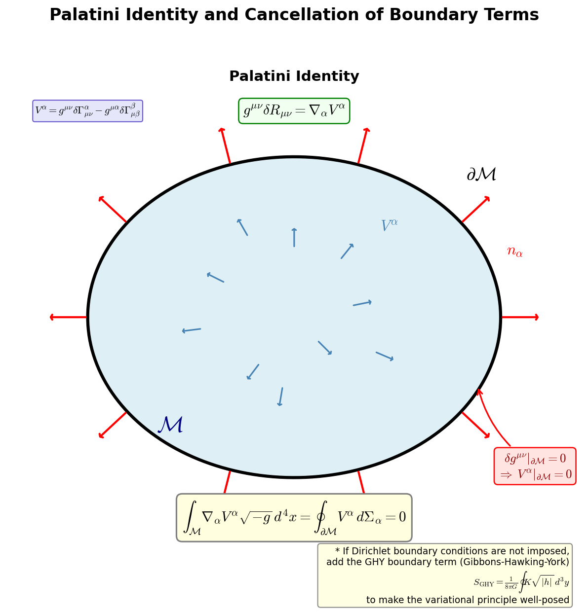
Fig. G.2: Process of Palatini's identity and boundary term cancellation. \(g^{\mu\nu}\delta R_{\mu\nu} = \nabla_\alpha V^\alpha\) becomes a boundary integral via the divergence theorem. Strictly, the addition of the Gibbons-Hawking-York boundary term is needed, but it does not affect the equations of motion
G.3.4: Combining the Three Contributions
🟡 Lina: Let's summarize. The three terms of \(\delta(\sqrt{-g}\,R)\) are:
- Term 1: \(\sqrt{-g}\,R_{\mu\nu}\,\delta g^{\mu\nu}\)
- Term 2: \(0\) (vanishes as a boundary term)
- Term 3: \(-\frac{1}{2}\sqrt{-g}\,R\,g_{\mu\nu}\,\delta g^{\mu\nu}\)
Therefore:
🔵 Kai: Because Term 2 vanishes, \(R_{\mu\nu} - \frac{1}{2}g_{\mu\nu}R\) comes together so cleanly. I can see the Einstein tensor taking shape!
🟡 Lina: Exactly. Now we just need to add the variation of the cosmological constant term:
Combining:
⚪ Mei: The variation of the gravitational part is now complete. All that's left is to add the matter action.
✅ Comprehension Check: According to the Palatini identity, in what form is \(\delta R_{\mu\nu}\) expressed?
Answer
It is expressed as a difference of covariant derivatives: \(\delta R_{\mu\nu} = \nabla_\alpha(\delta\Gamma^\alpha_{\mu\nu}) - \nabla_\nu(\delta\Gamma^\alpha_{\mu\alpha})\).
✅ Comprehension Check: Why does the \(g^{\mu\nu}\delta R_{\mu\nu}\) term ultimately not contribute?
Answer
Because it takes the form of a total derivative (\(\nabla_\alpha V^\alpha\)), which becomes a boundary term via the divergence theorem, and vanishes when \(\delta g^{\mu\nu} = 0\) on the boundary.
G.4: The Matter Action and the Energy-Momentum Tensor
G.4.1: Variational Definition of the Energy-Momentum Tensor
🟡 Lina: We vary the matter field action \(S_M[g^{\mu\nu}, \phi]\) with respect to the metric. Here \(\phi\) is a collective symbol representing matter fields (scalar fields, electromagnetic fields, etc.—all fields other than gravity). We'll see a concrete example shortly.
🟡 Lina: \(\frac{\delta S_M}{\delta g^{\mu\nu}}\) is called a functional derivative. Just as an ordinary derivative represents "the rate of change of a function when a variable is slightly changed," a functional derivative represents "the rate of change of the action (an integrated quantity) when the field \(g^{\mu\nu}(x)\) is slightly changed at each point" (see General Relativity General Relativity Appendix C).
🔵 Kai: An ordinary derivative is \(df/dx\), meaning "the rate of change of \(f\) when \(x\) is slightly moved," right? How is a functional derivative different?
🟡 Lina: In ordinary derivatives, there are finitely many variables (\(x\), \(y\), \(z\), etc.). In functional derivatives, the "variable" is the field \(g^{\mu\nu}(x)\)—meaning it has a value at each point in space. Imagine discretizing space into lattice points, treating \(g^{\mu\nu}\) at each point as an independent variable. In the discrete version, \(\delta S \approx \sum_i \frac{\partial S}{\partial g^{\mu\nu}_i}\,\delta g^{\mu\nu}_i\). As the lattice becomes infinitely fine, the sum \(\sum_i\) becomes an integral \(\int d^4x\), and the partial derivative \(\partial S/\partial g^{\mu\nu}_i\) gets replaced by the functional derivative \(\delta S_M/\delta g^{\mu\nu}(x)\).
⚪ Mei: So practically, we just need to write the variation of \(S_M\) in integral form and read off the coefficient of \(\delta g^{\mu\nu}\)?
🟡 Lina: Exactly right. The practical definition is precisely that: when we write the variation of \(S_M\) as
the coefficient multiplying \(\delta g^{\mu\nu}\) in the integrand is \(\frac{\delta S_M}{\delta g^{\mu\nu}}\)—this is the definition of the functional derivative. A note on notation: \(\delta S_M\) on the left side is "the infinitesimal change of the entire action," \(\delta g^{\mu\nu}\) on the right side is "the infinitesimal change of the metric," and \(\frac{\delta S_M}{\delta g^{\mu\nu}}\) is "the functional derivative." The same \(\delta\) is used throughout, but they are distinguished by context (same convention as writing \(df = \frac{df}{dx}\,dx\) in ordinary calculus, where \(d\) is used for both "total differential" and "differential operator"). We'll actually compute this in the scalar field example in G.4.3, so you can confirm the concrete procedure there.
🔵 Kai: Wait a moment. With an ordinary partial derivative, \(\partial f/\partial x_i\) means "move only \(x_i\) while holding everything else fixed," right? Is the functional derivative the same, meaning "change \(g^{\mu\nu}\) at only one point \(x\) while holding all other points fixed"?
🟡 Lina: Intuitively, yes. The functional derivative is the limit where lattice points become infinitely fine, and the notation uses \(\delta\) instead of \(\partial\) to distinguish it. However, in practice, rather than thinking of "moving just one point," the definition I just described—write \(\delta S_M\) in integral form and read off the coefficient of \(\delta g^{\mu\nu}\)—is easier to compute with. We'll use exactly that procedure in the scalar field example in G.4.3, so you'll get the feel for it there.
🔵 Kai: OK, let me confirm—with the definition you just gave, I write \(\delta S_M\) in integral form and read off the coefficient of \(\delta g^{\mu\nu}\), and that's \(\delta S_M/\delta g^{\mu\nu}\), right? Same structure as how in ordinary calculus, the coefficient in \(df = (\partial f/\partial x)\,dx\) is the derivative?
🟡 Lina: Perfect understanding. Exactly right. Now let me push one step further—what does it physically mean to vary the matter action "with respect to the metric"?
🔵 Kai: Hmm... "how much the matter is affected when you slightly change the shape of spacetime"? But wait, conversely, that's also an indicator of "how much the matter wants to curve spacetime," isn't it? Like action-reaction.
🟡 Lina: That's exactly the key point. How much the matter "resists" deformation of spacetime—quantifying the strength of that response gives the energy-momentum tensor. And that sits on the right side of the Einstein equations, becoming the source that determines the curvature of spacetime. Specifically, we define the energy-momentum tensor \(T_{\mu\nu}\) as follows:
Then:
🔵 Kai: Why the coefficient \(-2/\sqrt{-g}\)?
🟡 Lina: There are two reasons. First, with this coefficient, \(T_{00}\) exactly equals the energy density \(\rho\) in the Newtonian limit—we'll actually verify this in "G.5.3: Consistency with the Newtonian Limit". Second, the Einstein equations take the clean form \(G_{\mu\nu} = 8\pi G\,T_{\mu\nu}\). Also, the \(T_{\mu\nu}\) obtained with this definition is automatically a symmetric tensor (\(T_{\mu\nu} = T_{\nu\mu}\)). This generally differs from the canonical energy-momentum tensor obtained from Noether's theorem in Quantum Field Theory Quantum Field Theory Ch. 3, but this one is the physically correct one.
G.4.2: Concrete Example: Perfect Fluid
⚪ Mei: What specific \(T_{\mu\nu}\) comes out?
🟡 Lina: Let's look at two examples. First I'll just state the result for a perfect fluid—the variation of the fluid action is technically somewhat involved. After that, we'll trace through every step of the variation for a scalar field. The energy-momentum tensor for a perfect fluid is:
Here \(\rho\) is the energy density, \(p\) is the pressure, and \(u^\mu\) is the 4-velocity of the fluid.
To confirm that this comes from the variational definition, one varies the perfect fluid action \(S_M = -\int d^4x\,\sqrt{-g}\,\rho\) with respect to \(g^{\mu\nu}\) (for details, see the exercises in General Relativity General Relativity Appendix C).
G.4.3: Concrete Example: Scalar Field
🟡 Lina: The action for a scalar field \(\phi\) that we learned in Quantum Field Theory Quantum Field Theory Ch. 3:
We vary this with respect to \(g^{\mu\nu}\). Writing the integrand as \(\mathcal{L}_M\sqrt{-g}\):
🔵 Kai: The \(\delta\sqrt{-g}\) we computed in G.3.1 shows up again here.
🟡 Lina: Yes, the tools are reusable. First term: differentiating \(\mathcal{L}_M = -\frac{1}{2}g^{\alpha\beta}\partial_\alpha\phi\,\partial_\beta\phi - V(\phi)\) with respect to \(g^{\mu\nu}\):
Second term: using \(\delta\sqrt{-g} = -\frac{1}{2}\sqrt{-g}\,g_{\mu\nu}\,\delta g^{\mu\nu}\):
Combining:
Substituting into the definition \(T_{\mu\nu} = -\frac{2}{\sqrt{-g}}\frac{\delta S_M}{\delta g^{\mu\nu}}\):
🔵 Kai: This is the same form as the scalar field energy-momentum tensor we saw in Quantum Field Theory Quantum Field Theory Ch. 3!
🟡 Lina: Yes. Though in curved spacetime, \(\eta_{\mu\nu} \to g_{\mu\nu}\).
⚪ Mei: When you actually carry out the variational definition procedure—"write \(\delta S_M\) and read off the coefficient of \(\delta g^{\mu\nu}\)"—it comes out this straightforwardly.
✅ Comprehension Check: How is the energy-momentum tensor \(T_{\mu\nu}\) defined using the matter action \(S_M\)?
Answer
It is defined as \(T_{\mu\nu} \equiv -\frac{2}{\sqrt{-g}}\frac{\delta S_M}{\delta g^{\mu\nu}}\).
G.5: Completing the Einstein Equations
G.5.1: Derivation from the Variational Principle
🟡 Lina: Setting the variation of the total action \(S = S_{\text{grav}} + S_M\) to zero:
%%{init: {"theme": "default", "themeCSS": ".edgePath .path, .flowchart-link { stroke-width: 2px !important; }"}}%%
flowchart LR
    S["Total action S = S_grav + S_M"] --> SG["S_grav = 1/(16πG) ∫√-g (R-2Λ) d⁴x"]
    S --> SM["S_M[g, φ]"]
    SG -->|δ/δg^μν| LHS["(R_μν - ½g_μν R + Λg_μν) / (16πG)"]
    SM -->|δ/δg^μν| RHS["-½ T_μν"]
    LHS --> EQ["δS = 0"]
    RHS --> EQ
    EQ --> EINSTEIN["G_μν + Λg_μν = 8πG T_μν"]
Fig. G.3: Derivation from the variation of the total action to the Einstein equations
Since \(\delta g^{\mu\nu}\) is arbitrary, the integrand must vanish:
Multiplying by \(16\pi G\) and rearranging:
This is the Einstein equation with cosmological constant. Using the Einstein tensor \(G_{\mu\nu} \equiv R_{\mu\nu} - \frac{1}{2}g_{\mu\nu}R\):
🔵 Kai: We finally got it! Everything we computed by splitting into three parts in G.3 converges here and neatly becomes the Einstein equations.
⚪ Mei: It's the same form as the equation we saw in Ch. 6. Back then we accepted it without derivation, but now the same equation came out just by determining the action from four requirements and varying it—it's impressive that there was no point where we arbitrarily chose anything along the way.
G.5.2: Bianchi Identity and Energy Conservation
🟡 Lina: As a consistency check of the derivation, let's verify the Bianchi identity. As a purely geometrical identity from differential geometry (see General Relativity General Relativity Ch. 13):
This holds purely geometrically from the symmetries of the Riemann tensor. Combined with \(\nabla^\mu(\Lambda g_{\mu\nu}) = 0\) (since \(\nabla^\mu g_{\mu\nu} = 0\)):
The same condition is imposed on the right side of the Einstein equations:
🔵 Kai: Is \(\nabla^\mu T_{\mu\nu} = 0\) a generalization of \(\partial^\mu T_{\mu\nu} = 0\) (energy-momentum conservation) in flat spacetime? But in curved spacetime, the meaning of "conservation" seems to change...
🟡 Lina: Good intuition. In curved spacetime, \(\nabla^\mu T_{\mu\nu} = 0\) corresponds to a local conservation law. In flat spacetime, \(\nabla^\mu \to \partial^\mu\) and it reduces to ordinary energy-momentum conservation \(\partial^\mu T_{\mu\nu} = 0\). However, in curved spacetime, defining "the total amount of energy in the entire universe" is generally difficult—there's the problem of how to account for the energy of the gravitational field itself (see General Relativity General Relativity Ch. 15). We won't go into that here, but keep it in mind.
The important point is that this conservation law comes out automatically as a consequence of the Einstein equations. The general coordinate invariance of the action (\(S\) is invariant under coordinate transformations) guarantees \(\nabla^\mu T_{\mu\nu} = 0\) via Noether's theorem (see Quantum Field Theory Quantum Field Theory Ch. 3).
⚪ Mei: So there's no need to separately assume the conservation law—it comes out automatically from the symmetry.
🟡 Lina: Exactly. Note that the Bianchi identity \(\nabla^\mu G_{\mu\nu} = 0\) gives 4 identities for \(\nu = 0, 1, 2, 3\). The Einstein equations have 10 component equations due to the symmetry of \(g_{\mu\nu}\), but—
🔵 Kai: Wait. If 4 identities always hold, that means... 4 of the 10 components aren't independent?
🟡 Lina: Precisely. With 10 component equations and 4 Bianchi identities, there are 6 independent equations. This matches the 6 degrees of freedom obtained by subtracting 4 coordinate freedoms from the 10 components of the metric \(g_{\mu\nu}\).
🔵 Kai: Hm? What does "subtracting coordinate freedoms" mean? I remember from electromagnetism that the 4 components of \(A_\mu\) minus gauge degrees of freedom reduce the physical degrees of freedom (Quantum Field Theory Quantum Field Theory Ch. 3). Is this similar?
🟡 Lina: Exactly so. In electromagnetism, there's 1 gauge freedom \(A_\mu \to A_\mu + \partial_\mu\chi\), giving 4 components minus 1 = 3 degrees of freedom—and further, the constraint from the equations of motion physically gives 2 degrees of freedom for transverse waves. Maxwell's equations have 1 corresponding identity (\(\partial_\mu J^\mu = 0\)). For gravity, there are 4 coordinate transformation freedoms, giving 4 Bianchi identities. The structure is exactly the same. That is, both have a three-tier structure: "symmetry of the action → conservation law → consistency of the equations." In electromagnetism: gauge invariance → charge conservation → consistency of Maxwell's equations. In gravity: coordinate invariance → energy-momentum conservation → consistency of Einstein's equations.
🔵 Kai: So the larger the symmetry, the more identities there are, and the fewer independent equations. Electromagnetism has 1 identity giving \(4-1=3\), gravity has 4 identities giving \(10-4=6\)—same pattern.
🟡 Lina: Exactly. Symmetry "constrains" the theory. Summarizing quantitatively—in electromagnetism: "\(U(1)\) gauge invariance (1 parameter) → charge conservation (1 identity) → 3 independent equations out of 4 components." In gravity: "general coordinate invariance (4 parameters) → energy-momentum conservation (4 identities) → 6 independent equations out of 10 components."
⚪ Mei: To summarize: electromagnetism is "1-parameter symmetry → 1 identity → \(4-1=3\) independent equations," gravity is "4-parameter symmetry → 4 identities → \(10-4=6\) independent equations." The number of symmetry parameters directly becomes the number of identities.
🟡 Lina: That relationship is summarized in the diagram Fig. G.4 "Consistency between coordinate invariance and the Bianchi identity".
%%{init: {"theme": "default", "themeCSS": ".edgePath .path, .flowchart-link { stroke-width: 2px !important; }"}}%%
flowchart TD
    A["General coordinate invariance of action S"] -->|Noether's theorem| B["∇^μ T_μν = 0<br>(Energy-momentum conservation)"]
    A -->|Identity from differential geometry| C["∇^μ G_μν = 0<br>(Bianchi identity)"]
    C -->|LHS of Einstein equations| D["G_μν + Λg_μν = 8πG T_μν"]
    B -->|RHS of Einstein equations| D
    D --> E["Consistency of equations is guaranteed"]
Fig. G.4: Consistency between coordinate invariance and the Bianchi identity
🟡 Lina: Yes. This is the power of the action principle.
G.5.3: Consistency with the Newtonian Limit
🟡 Lina: Let's confirm that the coefficient \(8\pi G\) is correct. In a weak gravitational field:
Consider static, non-relativistic matter (\(T^{00} \approx \rho\), other components approximately zero, \(c = 1\)). Lowering the indices gives \(T_{00} = g_{0\alpha}g_{0\beta}T^{\alpha\beta}\). In the weak-field approximation, \(g_{0i} \approx 0\) and \(T^{0i} \approx 0\), \(T^{ij} \approx 0\), so the only surviving term in the sum is \(\alpha = 0\), \(\beta = 0\): \(T_{00} \approx g_{00}g_{00}T^{00} \approx (-1)(-1)\rho = \rho\).
🔵 Kai: Why is \(T^{0i} \approx 0\)? The energy density isn't zero, but the momentum density is?
🟡 Lina: "Non-relativistic" means the matter is nearly at rest. \(T^{0i}\) is the momentum density—corresponding to the speed of matter flow. If the matter isn't moving, the momentum density is zero. In the static, non-relativistic limit, the pressure is also zero, so \(T_{00} \approx \rho\) and other components are negligible.
⚪ Mei: We're checking whether we can reproduce the Newtonian limit by considering only "nearly stationary matter."
🟡 Lina: Right. Using the Einstein equation directly for the \(00\) component gives \(R_{00} - \frac{1}{2}g_{00}R = 8\pi G\,\rho\), but it's more transparent to first take the trace to eliminate \(R\).
Step 1: Taking the trace
Multiplying both sides of the Einstein equation \(G_{\mu\nu} = 8\pi G\,T_{\mu\nu}\) by \(g^{\mu\nu}\). The left side is \(g^{\mu\nu}G_{\mu\nu} = g^{\mu\nu}R_{\mu\nu} - \frac{1}{2}g^{\mu\nu}g_{\mu\nu}R = R - \frac{1}{2}\cdot 4 \cdot R = R - 2R = -R\). The right side is \(8\pi G\,g^{\mu\nu}T_{\mu\nu} = 8\pi G\,T\) (where \(T \equiv g^{\mu\nu}T_{\mu\nu}\) is the trace of the energy-momentum tensor). Therefore:
🔵 Kai: \(g^{\mu\nu}g_{\mu\nu} = 4\) because it's 4 dimensions?
🟡 Lina: Yes. \(g^{\mu\nu}g_{\mu\nu} = \delta^\mu_\mu = 4\) (in \(D\) dimensions it would be \(D\)).
Step 2: Trace-reversed form
Substituting this back into the original equation \(R_{\mu\nu} - \frac{1}{2}g_{\mu\nu}R = 8\pi G\,T_{\mu\nu}\) to eliminate \(R\):
This form is called the trace-reversed form.
Step 3: Taking the \(00\) component
For static, non-relativistic matter, \(T_{00} \approx \rho\). Setting \(p = 0\) in the perfect fluid formula gives \(T_{ij} = \rho\,u_i u_j\), but in the non-relativistic limit \(u_i \approx 0\) (same argument as before), so \(T_{ij} \approx 0\). Also, non-relativistic means \(u^i \approx 0\) (matter is nearly at rest). Substituting the weak-field approximation \(g_{00} \approx -1\), \(u^i \approx 0\) into the normalization condition for 4-velocity \(g_{\mu\nu}u^\mu u^\nu = -1\) gives \(-u^0 u^0 \approx -1\), so \(u^0 \approx 1\). Using the formula from G.4.2, \(T_{0i} = (\rho + p)u_0 u_i + p\,g_{0i}\). Since \(p = 0\), the second term vanishes. The first term contains \(u_i\), but lowering the index: \(u_i = g_{i\mu}u^\mu = g_{i0}u^0 + g_{ij}u^j\). In the weak-field approximation \(g_{i0} \approx 0\), and in the non-relativistic limit \(u^j \approx 0\), so even though \(u^0 \approx 1\), we have \(u_i \approx 0\). Therefore \(T_{0i} \approx 0\). In the weak-field approximation \(g^{\mu\nu} \approx \eta^{\mu\nu}\), so with the sign convention \((-,+,+,+)\): \(g^{00} \approx \eta^{00} = -1\), \(g^{0i} \approx \eta^{0i} = 0\), \(g^{ij} \approx \eta^{ij} = \delta^{ij}\). Therefore the trace is \(T = g^{\mu\nu}T_{\mu\nu}\). By the contraction rule, running \(\mu, \nu\) from 0 to 3: \(T = \sum_{\mu=0}^{3}\sum_{\nu=0}^{3} g^{\mu\nu}T_{\mu\nu}\). Splitting by values of \(\mu, \nu\): \(T = g^{00}T_{00} + g^{0i}T_{0i} + g^{i0}T_{i0} + g^{ij}T_{ij}\) (where \(i\) runs over 1, 2, 3). Due to symmetry \(g^{0i} = g^{i0}\), \(T_{0i} = T_{i0}\), the 2nd and 3rd terms have the same value, so \(T = g^{00}T_{00} + 2g^{0i}T_{0i} + g^{ij}T_{ij}\). With weak-field approximation \(g^{00} \approx -1\), \(g^{0i} \approx 0\), \(g^{ij} \approx \delta^{ij}\), and \(T_{00} \approx \rho\), \(T_{0i} \approx 0\), \(T_{ij} \approx 0\):
🔵 Kai: The trace being \(-\rho\) is because the sign of \(g^{00} = -1\) comes in.
🟡 Lina: Exactly. Since \(g_{00} \approx -1\) (in the weak-field approximation \(|\Phi| \ll 1\), \(-(1+2\Phi) \approx -1\)), the \(00\) component of the trace-reversed form's right side is \(8\pi G(T_{00} - \frac{1}{2}g_{00}T)\). Substituting \(T_{00} \approx \rho\), \(g_{00} \approx -1\), \(T \approx -\rho\):
Step 4: Writing the left side \(R_{00}\) in terms of the Newtonian potential
In the linear approximation, \(R_{00} \approx -\frac{1}{2}\nabla^2 h_{00}\) (see General Relativity General Relativity Ch. 8). In the weak-field approximation, \(g_{00} \approx -(1+2\Phi)\) (where \(\Phi\) is the Newtonian potential, \(|\Phi| \ll 1\)), so:
Substituting:
Step 5: Poisson's equation
Equating Steps 3 and 4:
🔵 Kai: Oh, that's Newton's Poisson equation! The Einstein equations reduce to Newtonian gravity!
🟡 Lina: This is exactly Newton's Poisson equation. The coefficient match confirms \(8\pi G\).
📝 Exercises:
- Verification of the Newtonian limit → Problem M-2. Newtonian Limit of Einstein-Hilbert
✅ Comprehension Check: Write the Einstein equation (with cosmological constant) obtained from the derivation.
Answer
\(R_{\mu\nu} - \frac{1}{2}g_{\mu\nu}R + \Lambda g_{\mu\nu} = 8\pi G\,T_{\mu\nu}\) (in natural units \(c=1\)).
✅ Comprehension Check: What condition determines the coefficient \(8\pi G\) on the right side of the Einstein equations?
Answer
It is determined by the condition that the equation reduces to Newton's Poisson equation \(\nabla^2\Phi = 4\pi G\rho\) in the weak gravitational field limit.
G.6: Meaning of the Derivation and Outlook Toward String Theory
G.6.1: The Power of the Action Principle
🟡 Lina: Let's summarize what this derivation shows.
- The Einstein equations didn't "fall from the sky" — They necessarily emerge from the variation of the simplest generally coordinate-invariant action \(\int\sqrt{-g}\,R\,d^4x\)
- Symmetry determines the equations — The requirements "generally coordinate-invariant," "constructed from the metric and its derivatives only," "up to second-order derivatives," and "simplest possible" almost uniquely determine the form of the action (up to the freedom of the cosmological constant)
- Conservation laws are automatically guaranteed — Symmetry of the action → Bianchi identity → \(\nabla^\mu T_{\mu\nu} = 0\)
- Starting point for quantization — The path integral \(\int\mathcal{D}[g]\,e^{iS_{EH}/\hbar}\) is (despite ultraviolet divergence issues) the formal starting point for quantum gravity
🔵 Kai: Point 2 is amazing. "If you determine the symmetry, the equation is determined"—conversely, if you get the symmetry wrong, everything goes wrong.
🟡 Lina: Exactly. That's why "finding the right symmetry" becomes the most important step in theory construction. Historically, Maxwell organized electromagnetism with gauge symmetry, Einstein demanded general coordinate invariance, and Yang-Mills introduced non-abelian gauge symmetry—in each case, the discovery of the symmetry was the decisive advance. And the larger the symmetry, the more the theory's freedom is reduced and the equations are constrained—if the symmetry is insufficient, there are too many candidates and nothing is uniquely determined.
⚪ Mei: So the action being almost uniquely determined by those 4 requirements was because the constraints from symmetry were so strong.
🟡 Lina: Exactly. Specifically, general coordinate invariance is a much larger symmetry than Lorentz invariance, so it strongly constrains the allowed forms of the action. For example, trying to describe gravity with only Lorentz invariance gives insufficient symmetry for a consistent theory. The Bianchi identities we saw in G.5.2 are also a concrete example of this "constraining"—symmetry generated 4 identities, reducing independent equations from 10 to 6.
G.6.2: Connection to String Theory {#string-appendix-g-connection-to-string-theory}}
🔵 Kai: What happens in string theory?
🟡 Lina: The Polyakov action we'll see in Ch. 13:
is the action of scalar fields \(X^\mu\) on the 2-dimensional worldsheet, where the worldsheet metric \(h_{ab}\) enters as an independent dynamical variable. What it shares with the Einstein-Hilbert action is the structure of "varying an action containing a metric with respect to that metric." \(h_{ab}\) is the worldsheet metric, and \(X^\mu\) are the embedding coordinates (functions telling where each point on the string is located in spacetime—introduced in detail in Ch. 13).
🔵 Kai: Varying with respect to \(g^{\mu\nu}\) to get \(T_{\mu\nu}\) in G.4, and varying with respect to \(h^{ab}\), is exactly the same spirit.
🟡 Lina: Exactly.
%%{init: {"theme": "default", "themeCSS": ".edgePath .path, .flowchart-link { stroke-width: 2px !important; }"}}%%
flowchart TD
    subgraph GR["General Relativity (4D spacetime)"]
        A1["Dynamical variable: g_μν"] --> A2["Action: S_EH = ∫d⁴x √-g R"]
        A2 -->|δ/δg^μν = 0| A3["Einstein equations"]
    end
    subgraph ST["String Theory (2D worldsheet)"]
        B1["Dynamical variables: h_ab, X^μ"] --> B2["Action: S_P = -T/2 ∫d²σ √-h h^ab ∂_a X^μ ∂_b X_μ"]
        B2 -->|δ/δh^ab = 0| B3["Constraint T_ab = 0"]
        B2 -->|δ/δX^μ = 0| B4["Wave equation"]
    end
    GR -.->|"Same spirit of variational principle<br>Dimension: 4→2"| ST
Fig. G.5: Structural similarity between the gravitational action and the string action
The spirit of variation is exactly the same: - Varying with respect to \(h^{ab}\) → Energy-momentum tensor on the worldsheet \(= 0\) (constraint) - Varying with respect to \(X^\mu\) → Equation of motion for the string (wave equation)
🔵 Kai: So varying the worldsheet metric \(h_{ab}\) corresponds to varying \(g_{\mu\nu}\) in the Einstein equations (Fig. G.5 "Structural similarity between the gravitational action and the string action").
⚪ Mei: Just changing the dimension from 4 to 2, but the procedure is the same.
🟡 Lina: Yes. Furthermore, the low-energy effective action of string theory yields the Einstein equations in higher dimensions (+ higher-order corrections). In other words, string theory "contains" Einstein's gravity. This is one of the reasons string theory is considered a candidate for quantum gravity.
G.6.3: A Note on Philosophy of Science
🟡 Lina: One final point. This derivation is beautiful, but there's something we must not forget.
The Einstein equations are a model. Choosing "the simplest action" was a human aesthetic judgment, and there's no guarantee that nature follows it. In fact:
- At high energies, \(R^2\) terms or \(R_{\mu\nu}R^{\mu\nu}\) terms might become important (higher-derivative gravity models)
- Quantum effects might modify the action itself
- String theory predicts infinitely many higher-order corrections in an expansion in \(\alpha'\) (the inverse of string tension)
🔵 Kai: So the Einstein equations aren't "correct"—they're "the simplest model that currently agrees with experiment"?
🟡 Lina: Exactly. Choosing the action as "the simplest" is justified because it's correct within the range verifiable by current experimental precision. But it's not an eternal truth—there's always the possibility of modification by more precise experiments.
🔵 Kai: If in the future, more precise observations found an \(R^2\) term, would we just need to rewrite the action?
🟡 Lina: Precisely. We keep the framework of the action principle and modify the contents of the action. This is another advantage of the action principle—theoretical extensions can be done systematically. The variational procedure itself doesn't change; only the contents are replaced. In other words, the action principle provides not "the answer" but "a way of framing the question"—the contents are determined by experiment. The strength of physics is that it always maintains "falsifiability" in the philosophy of science sense—the possibility of being refuted by experiment. Never forget the attitude of judging for yourself.
⚪ Mei: I see—the framework is fixed while the contents are swapped—so even when adding an \(R^2\) term, you still do the same thing: "vary and set to zero."
📝 Exercises:
- Variation with the cosmological constant term added → Problem M-3. Variation of the Cosmological Constant Term
✅ Comprehension Check: Why is \(R\) (scalar curvature) chosen as the action?
Answer
Because \(R\) is the simplest generally coordinate-invariant scalar containing second-order derivatives of the metric tensor. However, this is a choice based on the aesthetic judgment of "simplest possible," and it may be modified at high energies.
G.7: Practice Problems
Here we re-list the practice problems that appeared in this appendix.
📝 Exercises:
- Derivation of \(\delta\sqrt{-g}\) → Problem M-1. Derivation of \(\delta\sqrt{-g}\)
- Verification of the Newtonian limit → Problem M-2. Newtonian Limit of Einstein-Hilbert
- Variation with the cosmological constant term added → Problem M-3. Variation of the Cosmological Constant Term
Preview of Next Chapter
In this appendix, we completed the variational derivation of the Einstein equations. In Ch. 13, we apply the same spirit of the variational principle to strings, deriving the equations of motion and constraint conditions from the Polyakov action.
References
- Sean Carroll, Spacetime and Geometry, Ch.4 "Derivation of the Einstein Equations" — Detailed discussion of Palatini's identity and boundary terms
- David Tong, Lectures on General Relativity, Ch.4: "The Einstein Equations" — Clear exposition of the variational calculation
- Robert Wald, General Relativity, Ch.E "Variational Principles" — Rigorous treatment of the Gibbons-Hawking-York boundary term
- Barton Zwiebach, A First Course in String Theory, Ch.12: "Relativistic quantum open strings" — Analogy between the string action and variation
- General Relativity Chapter 14 — Derivation of the Einstein equations (detailed version of equivalent content; readers who have already covered it may skip this appendix)
- General Relativity Appendix C — Variational calculus and the principle of least action
- Quantum Field Theory Chapter 3 — Classical field theory, Lagrangians, and Noether's theorem
Feedback on this page
Let us know if something was unclear, incorrect, or could be improved.