Appendix H: BRST Quantization and the bc Ghost System¶
Story so far: In Ch. 16 16.7 "CFT Re-derivation of the Critical Dimension", we derived the critical dimension \(D = 26\) of the bosonic string from the condition that "the sum of the matter field central charge \(c_{\text{matter}} = D\) and the ghost field central charge \(c_{\text{ghost}} = -26\) equals zero." However, in the main text \(c_{\text{ghost}} = -26\) was simply stated as a result with the note that "the calculation is technical." This appendix fills that gap.
Goals of this appendix
- Starting from the Faddeev-Popov procedure, derive why ghost fields \(b, c\) are necessary for quantizing string theory, how their energy-momentum tensor is determined, and why the \((z-w)^{-4}\) coefficient of the \(T_{\text{ghost}}\, T_{\text{ghost}}\) OPE gives \(c_{\text{ghost}} = -26\), at a level where every step of the algebra can be followed
On difficulty: This appendix is the most technical section in The Quest for Quantum Gravity. Several new concepts appear, including anticommuting fields (Grassmann fields), the Faddeev-Popov prescription, and Wick's theorem for anticommuting fields. On a first reading, we recommend "simply accepting the result \(c_{\text{ghost}} = -26\) and continuing with Ch. 16 16.7 "CFT Re-derivation of the Critical Dimension"." Come back when your curiosity draws you here.
Fig. H.1 "Logical flow of BRST quantization and the ghost central charge" shows the logical flow of this entire appendix. Follow along while checking which section corresponds to each step.
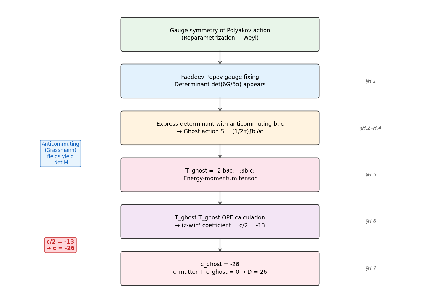
Fig. H.1: Logical flow of BRST quantization and the ghost central charge. Starting from the gauge symmetry of the Polyakov action, we proceed through the Faddeev-Popov procedure → introduction of bc ghost fields → energy-momentum tensor → TT OPE calculation → determination of c_ghost = -26.
H.1 The Need for Gauge Fixing — Motivation for Faddeev-Popov¶
🟡 Lina: The Polyakov action of string theory (Ch. 13) had three gauge symmetries—reparametrization invariance (two) and Weyl invariance (one). These represent "apparent differences in the same state" rather than "physically distinct states."
🔵 Kai: What's the problem with having gauge symmetry?
🟡 Lina: In the path integral \(Z = \int \mathcal{D}g\, \mathcal{D}X\, e^{iS}\), when we sum over all metrics \(g_{ab}\), we end up counting configurations related by gauge transformations—families of metrics that look different but are physically identical—infinitely many times over. Such "collections of physically identical configurations connected by gauge transformations" are called gauge orbits. To avoid this, we need the operation of "choosing exactly one representative from each gauge orbit"—gauge fixing.
Gauge Fixing and the Jacobian Factor¶
🟡 Lina: The standard prescription for gauge fixing is the Faddeev-Popov method. In essence, it's a generalization of the change-of-variables Jacobian from high school mathematics.
For example, when you want to integrate a two-variable function \(F(x, y)\) along the \(y\)-axis (\(x = 0\)):
The delta function "selects the representative \(x = 0\)." This is the prototype of gauge fixing.
🔵 Kai: Ah, so the delta function "picks out only the points satisfying the condition."
🟡 Lina: Right. In general, when we want to impose a gauge-fixing condition \(G(g) = 0\), we insert a delta function \(\delta[G(g)]\). However, to ensure we select exactly one representative from every gauge orbit, we need to attach the correct Jacobian factor.
Let's think by analogy with finite dimensions. Consider the one-variable case. Under the change of variables \(u = f(x)\), we have \(du = f'(x)\, dx\) so \(dx = du/|f'(x)|\). Using the delta function property \(\int du\, \delta(u) = 1\):
(when \(f(x) = 0\) has a single solution). That is, \(|f'(x)|\) is the Jacobian (the "stretch factor" of the variable change), and multiplying by it ensures that \(\delta(f(x))\) correctly "selects exactly one representative at \(f = 0\)."
⚪ Mei: It's the idea of substitution \(dx = du/f'(x)\) from high school, combined with the delta function.
🟡 Lina: Extending to multiple variables, for \(n\) conditions \(f_i(x_1, \ldots, x_n) = 0\) (\(i = 1, \ldots, n\)):
The Jacobian generalizes from \(|f'|\) to the determinant \(|\det(\partial f_i/\partial x_j)|\). Formally extending this to infinite dimensions (variables \(x_j\) → gauge parameter fields \(\alpha(\sigma)\), conditions \(f_i\) → gauge-fixing condition \(G\)):
Here \(g^\alpha\) denotes the gauge transformation by parameter \(\alpha\). In finite dimensions we had the absolute value \(|\det|\), but here we write \(\det\) without absolute value. The reason: as we'll see in the next subsection, this determinant is represented as a Gaussian integral over anticommuting fields (ghost fields). The Gaussian integral over anticommuting fields automatically gives \(\det M\) itself (including sign), so there's no need to take the absolute value separately—the sign information is correctly incorporated within the ghost field path integral. Inserting this "1" into the path integral, the Faddeev-Popov determinant \(\det(\delta G/\delta\alpha)\) appears.
Rewriting the Determinant as Ghost Fields¶
🟡 Lina: The core idea of Faddeev-Popov is to rewrite this determinant as a path integral over new integration variables.
🔵 Kai: Rewriting a determinant as an integral...? How does that work?
🟡 Lina: We use the properties of Grassmann (anticommuting) variables. Grassmann variables are special mathematical objects where "swapping two of them flips the sign," introduced to describe fermions (particles with half-integer spin like electrons). (The basic computational rules for anticommuting fields are summarized in Section H.3. For details on the definition and derivation of Grassmann integration, see Quantum Field Theory Quantum Field Theory Ch. 12.) The Gaussian integral of anticommuting variables \(\theta_i\) (\(\theta_i \theta_j = -\theta_j \theta_i\)) gives:
(In contrast to the ordinary real Gaussian integral which gives \((\det M)^{-1/2}\), anticommuting variables give \(\det M\) itself. Why? An anticommuting variable \(\theta\) satisfies \(\theta^2 = 0\), so any function of \(\theta\) is exhausted by \(f(\theta) = a + b\theta\) (second order and above vanish). Grassmann integration is defined as "the operation of extracting the coefficient of \(\theta\)": \(\int d\theta\, \theta = 1\), \(\int d\theta\, 1 = 0\). While ordinary integration "sums areas," Grassmann integration behaves like "differentiation," lowering powers. For this reason, the \(\det M\) that appears in the denominator for ordinary Gaussian integrals appears in the numerator for anticommuting variables. See Quantum Field Theory Quantum Field Theory Ch. 12 for details.)
⚪ Mei: With ordinary integration you get \((\det M)^{-1/2}\), but with anticommuting variables you get \(\det M\)—it's the inverse.
🟡 Lina: Therefore, the Faddeev-Popov determinant can be expressed as a path integral over anticommuting fields (ghost fields):
⚪ Mei: So ghost fields are not "physical particles" but "auxiliary fields for expressing the determinant as a path integral."
🟡 Lina: Exactly. That's why they're called "ghosts"—they don't physically exist but are necessary for the calculation.
✅ Comprehension Check: The Faddeev-Popov determinant can be expressed as a path integral over ghost fields because the integration variables possess what property?
Answer
Because the integration variables are anticommuting (Grassmann) variables. The Gaussian integral over anticommuting variables gives \(\det M\) (compared to \((\det M)^{-1/2}\) for ordinary real variables), which allows the Faddeev-Popov determinant to be expressed as a path integral over anticommuting fields \(b, c\).
H.2 Application to String Theory — The Emergence of the \(bc\) System¶
🟡 Lina: In the Polyakov action of string theory, the three gauge symmetries (two reparametrizations + Weyl) are used to fix the conformal gauge \(h_{ab} = \eta_{ab}\) (or \(h_{ab} = \delta_{ab}\) in the Euclidean version). The ghost fields that appear to handle the required Faddeev-Popov determinant are the \(b\) ghost and \(c\) ghost.
Omitting details, they are arranged as follows:
- \(c^a(z)\): anticommuting field (worldsheet vector) replacing the infinitesimal reparametrization parameter \(\delta\sigma^a\)
- \(b_{ab}(z)\): anticommuting field (symmetric traceless worldsheet tensor) appearing as the Lagrange multiplier for the Faddeev-Popov condition
In complex coordinates \(z, \bar{z}\), the independent components are:
- \(c(z)\) (holomorphic component), \(\bar{c}(\bar{z})\) (antiholomorphic component)
- \(b(z)\) (holomorphic component), \(\bar{b}(\bar{z})\) (antiholomorphic component)
In this appendix we treat only the holomorphic sector \((b, c)\). The antiholomorphic sector is treated in a completely parallel manner.
Determining the Conformal Weights¶
🟡 Lina: The conformal weights of the ghost fields are determined by the objects they originate from:
-
\(c^a\): The coordinate transformation parameter \(\delta\sigma^a\) is a vector (E.3 "Complex Coordinates \(z, \bar{z}\) and Differentiation"). In complex coordinates, let's see how \(\epsilon(z)\) transforms under \(z \to w = f(z)\).
First, consider a concrete example. For \(w = 2z\) (stretching the coordinate by a factor of 2), \(df/dz = 2\). The vector field \(v = \epsilon(z)\, \partial_z\) is a coordinate-independent geometric object—for example, the fact that "you're walking north at 5 km/h" doesn't change when you change the map's scale (coordinate system). Similarly, \(v\) is a quantity with "direction and magnitude" independent of the choice of coordinates—so in the new coordinate \(w\), the same \(v\) can be written as \(v = \tilde\epsilon(w)\, \partial_w\). Here \(\partial_z\) is a coordinate basis vector (see Ch. 6 6.2 "Summary of Key Points in General Relativity (What We Need for String Theory)"), and from the chain rule \(\partial_z = (df/dz)\, \partial_w\) holds. Intuitively, "moving \(z\) by 1 moves \(w\) by \(df/dz\)."
🔵 Kai: "Moving \(z\) by 1 moves \(w\) by 2," so even for the same vector, the component in \(w\) coordinates changes... right?
🟡 Lina: Exactly. Suppose at some point there's a vector \(v = 3\, \partial_z\) ("speed 3 in \(z\) coordinates"). In \(w\) coordinates the same vector is written \(v = \tilde\epsilon\, \partial_w\). Since \(\partial_z = (df/dz)\, \partial_w = 2\, \partial_w\), we get \(v = 3 \cdot 2\, \partial_w = 6\, \partial_w\), so \(\tilde\epsilon = 6 = 2 \cdot 3 = (df/dz) \cdot \epsilon\). In general, substituting the chain rule \(\partial_z = (df/dz)\, \partial_w\) gives \(\epsilon(z)\, (df/dz)\, \partial_w = \tilde\epsilon(w)\, \partial_w\), and comparing coefficients of \(\partial_w\): \(\tilde\epsilon(w) = (df/dz)\, \epsilon(z)\). Solving for \(\epsilon(z)\): \(\epsilon(z) = (df/dz)^{-1}\, \tilde\epsilon(f(z))\).
On the other hand, the transformation law for a primary field of conformal weight $h$ introduced in [Ch. 16](../../content_string/chapters/ch16.md) [16.4 "Operator Product Expansion (OPE)"](ch16.md#string-ch16-s4) was $\phi(z) = (df/dz)^h\, \tilde\phi(f(z))$. The meaning of this formula: it relates the field value $\phi(z)$ in coordinate $z$ to the field value $\tilde\phi(w)$ in the new coordinate $w = f(z)$. If $h > 0$, stretching the coordinate ($df/dz > 1$) makes the field value larger; if $h < 0$, smaller. The expression $\epsilon(z) = (df/dz)^{-1}\, \tilde\epsilon(f(z))$ obtained above is precisely this form with $h = -1$. Therefore the conformal weight of $c(z)$ is $h_c = -1$.
⚪ Mei: The exponent is \(-1\) so the conformal weight is \(-1\)—the form of the transformation law directly tells us the answer.
🟡 Lina: Now let's look at the \(b\) side.
- \(b_{ab}\): The \(b_{zz}(z) \equiv b(z)\) component of the symmetric traceless tensor \(b_{ab}\) is a tensor of weight \(h_b = +2\). Let's see why. In the action, \(b_{zz}\) appears as the Lagrange multiplier for the gauge-fixing condition \(\delta g_{zz} = 0\) in the form \(\int d^2z\, b_{zz}\, \delta g_{zz}\). For this integral to be invariant under coordinate transformations, \(b_{zz}\) and \(\delta g_{zz}\) must have the same conformal weight. The weight of \(\delta g_{zz}\) is determined from the transformation of the \(zz\) component of the metric tensor: under \(z \to w = f(z)\), \(g_{zz} = (df/dz)^2\, \tilde g_{ww}\) (the index \(z\) appears twice, so \((df/dz)\) is multiplied twice). This is precisely the transformation law for conformal weight \(h = 2\). Therefore \(h_b = 2\).
🔵 Kai: Weight \(h_b = 2\), \(h_c = -1\), so their sum is \(h_b + h_c = 1\).
🟡 Lina: That "1" will matter later—written as a differential form, the action has the form \(b\, dc \cdot dz\, d\bar{z}\), so integrability requires the sum of weights to be 1.
✅ Comprehension Check: In the \(bc\) ghost system of string theory, what are the conformal weights of \(b(z)\) and \(c(z)\) respectively? And what physical objects do they originate from?
Answer
The conformal weight of \(b(z)\) is \(h_b = 2\) (originating from the Lagrange multiplier for the symmetric traceless metric variation \(\delta g_{zz}\)), and the conformal weight of \(c(z)\) is \(h_c = -1\) (originating from the coordinate transformation parameter \(\delta z = \epsilon(z)\)). Their sum is \(h_b + h_c = 1\).
H.3 Basics of Anticommuting Fields (Grassmann Fields)¶
🟡 Lina: Ghost fields are anticommuting fields, handled with different rules from bosonic fields. Let's summarize the basics here. For details, see Quantum Field Theory Chapters 5 and 12.
Anticommutation Relations¶
🟡 Lina: Anticommuting fields \(\psi(z), \chi(w)\) satisfy:
In particular, the square of the same field vanishes: \(\psi(z)^2 = 0\).
Normal Ordering and Contractions¶
🟡 Lina: In normal ordering \(:bc:\) for anticommuting fields, a minus sign appears when exchanging operators:
The fundamental contraction values (derived in the next section):
Here \(\langle \cdots \rangle\) denotes the expectation value under radial ordering. Radial ordering is a convention for defining products of fields in two-dimensional conformal field theory: "place the field with larger distance \(|z|\) from the origin on the left" (see Ch. 16 16.4 "Operator Product Expansion (OPE)"). When \(|z| > |w|\), both \(b(z)c(w)\) and \(c(z)b(w)\) already satisfy the radial ordering condition "larger \(|z|\) on the left," so they are evaluated in their given order.
The reason both contraction values equal \(1/(z-w)\): \(\langle b(z) c(w)\rangle\) is the propagator \(G_{bc}(z,w) = 1/(z-w)\) determined from the action. Meanwhile \(\langle c(z) b(w)\rangle\) is \(G_{cb}(z,w)\), and when independently derived in Section H.4, it also gives \(1/(z-w)\). You might think "shouldn't there be a minus sign since they anticommute?" but the radially ordered expectation value does not involve reordering the fields—it's simply the result of the path integral under the condition \(|z| > |w|\). The contraction values themselves are c-numbers (ordinary numbers) and are unaffected by anticommutation relations.
Wick's Theorem for Anticommuting Fields¶
🟡 Lina: Wick's theorem for anticommuting fields has an additional rule compared to the bosonic case: "a minus sign for each crossing of contraction lines." Specifically, the sign is determined by the parity of "how many fields you had to pass through to bring the two contracted fields next to each other."
Let me give an example. Suppose four anticommuting fields \(A\, B\, C\, D\) are lined up, and you want to contract \(A\) with \(C\), and \(B\) with \(D\). The sign is determined by "the number of crossings of contraction lines": if you draw arcs above the original ordering for the \(A\)-\(C\) contraction and the \(B\)-\(D\) contraction, the two arcs cross once. The total crossing count is 1 (odd), so the sign is \((-1)^1 = -1\).
An alternative way to see it: to bring \(A\) and \(C\) next to each other, you hop over the intervening \(B\) once (anticommutation gives sign \(-1\)). After that, \(B\) and \(D\) are already adjacent, so no additional sign. Either method gives the same result.
🔵 Kai: Drawing arcs and counting crossings seems more visual than rearranging fields in your head.
🟡 Lina: Another example: for \(A\, B\, C\, D\), contract \(A\) with \(D\) and \(B\) with \(C\). Drawing the \(A\)-\(D\) arc and the \(B\)-\(C\) arc, the \(B\)-\(C\) arc fits inside the \(A\)-\(D\) arc without crossing. Crossing count 0 (even), so the sign is \((-1)^0 = +1\). In Section H.6, the pattern \((1,4)(2,3)\) appearing in term (I) is precisely this "\(A\) with \(D\), \(B\) with \(C\)" form—drawing arcs, the \((2,3)\) arc fits inside the \((1,4)\) arc without crossing. Crossing count 0, sign \((-1)^0 = +1\).
However, from Section H.5 onward we deal with contractions of normal-ordered products \(:\!b\partial c\!:(z)\) with external fields \(c(w)\), and in Section H.6 with contractions between \(:\!b\partial c\!:(z)\, :\!b\partial c\!:(w)\). For contractions between normal-ordered products, the number of hops needed to "extract a field from the normal-ordered product" also affects the sign. The specific prescriptions are demonstrated with examples in Sections H.5 and H.6.
For the calculations in this appendix, it suffices to remember only the frequently used rules:
-
Sign rule for contractions between normal-ordered products: In \(:\!A\, B\!:\, :\!C\, D\!:\), to contract \(A\) with \(D\), you need to "extract" \(D\) from the right normal-ordered product by hopping over \(C\) (1 hop → sign \(-1\)). In general, count the number of anticommuting fields hopped over to move the contracted field to the edge of the normal-ordered product, and the sign is \((-1)^{\text{number of hops}}\).
Approach in this appendix: Section H.5 deals with the \(T\)-\(c\) OPE (partial contractions), where the above "core rule" alone is sufficient to completely track signs. However, in Section H.6's \(TT\) OPE (full contractions between normal-ordered products), additional sign rules are needed that go beyond this appendix's scope (see Polchinski Vol.1 §2.5, §3.3). Therefore in Section H.6 we focus on tracking the absolute values of each term's contribution, and determine the overall sign to be \(-13\) from the physical argument that "fermion loops produce a \((-1)\)" (details in Section H.6). 2. Contraction of \(b\) inside \(:bc:\) with external \(c\): A special case of the above rule. If \(b\) is at the left edge of the normal-ordered product, 0 hops means \(+\). 3. Square-like terms of the same field: Often vanish using \(\psi(z)^2 = 0\).
🔵 Kai: So in the H.6 calculation, when four fields are lined up, "which field you contract with which" changes the hop count, and that affects the sign.
🟡 Lina: Exactly.
H.4 The Action and Fundamental OPE of the \(bc\) System¶
Derivation of the Action¶
🟡 Lina: Following the Faddeev-Popov procedure carefully, the ghost action in conformal gauge for string theory takes the form:
Extracting the holomorphic sector alone: \(S^+ = \frac{1}{2\pi}\int d^2z\, b\, \bar\partial c\).
🔵 Kai: Since \(\bar\partial c\) appears in the action, the equation of motion must be \(\bar\partial c = 0\).
🟡 Lina: Right. Varying with respect to \(c(z)\) gives the equation of motion for \(b\), and varying with respect to \(b(z)\) gives that for \(c\):
So both \(c\) and \(b\) are holomorphic functions. This fits naturally within the framework of conformal field theory.
Derivation of the Fundamental OPE¶
🟡 Lina: Let's find the correlation function (propagator, also called the Green's function) between the two fields. In the action \(S = \frac{1}{2\pi}\int d^2z\, b\, \bar\partial c\), the equation of motion for \(c\) obtained by varying \(b\) is \(\bar\partial c = 0\) (similarly, varying \(c\) gives \(\bar\partial b = 0\)).
The propagator \(G(z,w) = \langle c(z)\, b(w)\rangle\) is defined as the solution of "the equation of motion with a point source." In path integral language, \(\langle c(z)\, b(w)\rangle\) represents "how \(c\) responds when \(b\) is inserted at \(w\)." Specifically, under the action \(S = \frac{1}{2\pi}\int d^2z\, b\, \bar\partial c\), using a path integral identity (Schwinger-Dyson equation), \(G(z,w)\) satisfies the differential equation:
Let's see where this equation comes from. In the path integral \(\langle c(z)\, b(w)\rangle = \int \mathcal{D}b\, \mathcal{D}c\; c(z)\, b(w)\, e^{-S}\), taking the functional derivative with respect to \(b(z)\) (using \(\delta S/\delta b(z) = 0\) inside the path integral—this is the quantum version of the classical equation of motion, called the Schwinger-Dyson equation) extracts the operator \(\frac{1}{2\pi}\bar\partial_z\) acting on \(c(z)\), with a delta function appearing on the right-hand side. That is, the \(1/(2\pi)\) is the coefficient of the kinetic term in the action inherited directly by the differential equation.
🔵 Kai: This has the same structure as solving \(\nabla^2 \phi = -\rho\) for Coulomb's law in electromagnetism. A delta function appears at the point charge, and the solution gives the potential.
🟡 Lina: Good analogy. We use the relation derived in E.8 "Green's Function for the 2D Free Field". For the normalization \(\int dx\, dy\, \delta_{xy}^{(2)}(z-w) = 1\) in real coordinates \((x,y)\), we have \(\partial_{\bar{z}}(1/(z-w)) = \pi\delta_{xy}^{(2)}(z-w)\) (E.8 "Green's Function for the 2D Free Field").
The action in this appendix is written as \(\frac{1}{2\pi}\int d^2z\, (\cdots)\). In the standard string theory convention, \(d^2z \equiv 2\, dx\, dy\) (Polchinski Vol.1 (2.1.6)), and using the delta function \(\delta^{(2)}\) normalized with respect to this measure (\(\int d^2z\, \delta^{(2)} = 1\)), the result from E.8 "Green's Function for the 2D Free Field" can be rewritten as:
(Derivation: Since \(d^2z = 2\,dx\,dy\), \(\int d^2z\, \delta^{(2)} = 1\) means \(\int 2\,dx\,dy\, \delta^{(2)} = 1\). Since \(\int dx\,dy\, \delta_{xy}^{(2)} = 1\), we get \(\delta^{(2)} = \frac{1}{2}\delta_{xy}^{(2)}\). Substituting E.8 "Green's Function for the 2D Free Field"'s \(\partial_{\bar{z}}(1/(z-w)) = \pi\delta_{xy}^{(2)} = 2\pi\delta^{(2)}\) gives the above.) Therefore:
Substituting into the left-hand side gives \(\frac{1}{2\pi}\cdot 2\pi\delta^{(2)}(z-w) = \delta^{(2)}(z-w)\), which indeed holds.
⚪ Mei: When you match the measure conventions correctly, the \(2\pi\) cancels cleanly.
🟡 Lina: Although these are anticommuting fields, under radial ordering:
(\(\sim\) denotes equality of the singular part of the OPE. The remainder is regular.)
🔵 Kai: The OPE for the bosonic field \(\partial X \partial X\) was \(1/(z-w)^2\), but for \(bc\) it's \(1/(z-w)\)—one degree less singular. What creates the difference?
🟡 Lina: The structure of the action is different. The \(bc\) system action is \(b\, \bar\partial c\), with only one derivative between \(b\) and \(c\). So the propagator is \(1/(z-w)\). On the other hand, the bosonic field action is \(\partial X\, \bar\partial X\) with two derivatives, so the \(X(z)X(w)\) propagator is \(\ln|z-w|^2\), and the \(\partial X\, \partial X\) OPE becomes \(1/(z-w)^2\) after differentiating twice.
✅ Comprehension Check: The fundamental OPE \(b(z)c(w) \sim 1/(z-w)\) of the \(bc\) system is derived from what structure in the action?
Answer
From the action \(S = \frac{1}{2\pi}\int d^2z\, b\, \bar\partial c\), the propagator equation \(\frac{1}{2\pi}\bar\partial_z G(z,w) = \delta^{(2)}(z-w)\) is obtained, and using the relation \(\bar\partial_z(1/(z-w)) = 2\pi\delta^{(2)}(z-w)\), we derive \(G(z,w) = \langle c(z)b(w)\rangle = 1/(z-w)\).
H.5 The Energy-Momentum Tensor of the \(bc\) System¶
Determining the Energy-Momentum Tensor¶
🟡 Lina: The energy-momentum tensor of the \(bc\) system with action \(S = \frac{1}{2\pi}\int d^2z\, b\, \bar\partial c\) can be derived from Noether's theorem (translational symmetry). However, since the Noether procedure for anticommuting fields is technical, here we'll understand the result through a different approach—the consistency condition that "the OPE of \(T\) with each field reproduces the correct conformal weight."
The result, with \(\lambda\) denoting the conformal weight of \(b\) (so \(c\) has weight \(1-\lambda\)), is:
We write this for general \(\lambda\) because in Section H.7 we'll use it to obtain the central charge for various systems (free fermions, superstring ghosts, etc.) at once by varying \(\lambda\).
🔵 Kai: So the content of \(T\) changes when the weight \(\lambda\) changes. What does it look like specifically for string theory where \(\lambda = 2\)?
🟡 Lina: Correspondence with literature sign conventions: In Polchinski Vol.1 (2.5.11), it's written as \(T = -:(\partial b)c: + \lambda\, \partial(:bc:)\) (Polchinski's \(\lambda\) is the weight of \(c\), corresponding to \(1-\lambda\) in this appendix). Replacing Polchinski's \(\lambda\) with \(1-\lambda\) to match our convention \(\lambda = h_b\) gives \(T = -:(\partial b)c: + (1-\lambda)\, \partial(:bc:)\), and substituting \(\partial(:bc:) = :(\partial b)c: + :b(\partial c):\) and expanding: \(T = -:(\partial b)c: + (1-\lambda):(\partial b)c: + (1-\lambda):b(\partial c): = -\lambda:(\partial b)c: + (1-\lambda):b(\partial c):\). Noting that within normal-ordered products \(:b(\partial c): = -:(\partial c)b:\), this agrees with our \(T_{\text{ghost}} = -\lambda :b\,\partial c: + (1-\lambda) :\partial b\, c:\) (since \(:(\partial b)c: = :\partial b\, c:\)). Below we verify that the OPE reproduces the correct conformal weights under this definition.
For string theory, \(\lambda = 2\) (the weight of \(b\)), so \(-\lambda = -2\) and \((1-\lambda) = 1-2 = -1\). Substituting into the general formula:
🔵 Kai: Why does it take this form?
🟡 Lina: It's determined by the condition that the OPE of \(T_\text{ghost}(z)\) with \(b(w)\) and \(c(w)\) makes "\(b\) behave as a primary field of weight \(\lambda\)" and "\(c\) behave as a primary field of weight \(1-\lambda\)." That is, we assume the form of \(T\), compute the OPE, and verify that the correct conformal weights are reproduced—this agrees with the result from Noether's theorem.
We'll now do one verification calculation. The OPEs that the correct \(T_{\text{ghost}}\) must satisfy are:
The simplest quadratic expression satisfying these conditions is the above \(T_{\text{ghost}}\). Let's verify one of them. We compute the OPE \(T_{\text{ghost}}(z)\, c(w)\). In the OPE of the first term \(-\lambda\, :\!b\partial c\!:(z)\) with \(c(w)\), only the contraction \(\langle b(z)c(w)\rangle = 1/(z-w)\) contributes (the contraction \(\langle cc\rangle = 0\) vanishes), leaving \(\partial c(z)\). Expanding \(\partial c(z) = \partial c(w) + (z-w)\partial^2 c(w) + \cdots\), the first term gives \(-\lambda\, \partial c(w)/(z-w)\). In the second term \((1-\lambda)\, :\!\partial b\, c\!:(z)\), we consider the contraction of \(\partial b(z)\) with the external \(c(w)\).
Here we split the calculation into two stages. In Stage 1, we compute naively "ignoring the additional \((-1)\) from extracting a field from a normal-ordered product" and confirm that the result is wrong. In Stage 2, we redo it with the correct rule.
What we "ignore" in Stage 1 is only the sign arising from rearranging anticommuting fields; signs arising from differentiation are always included. This distinction is important:
- Signs from contraction values: Signs resulting from differentiation (e.g., \(\partial_z(1/(z-w)) = -1/(z-w)^2\)) → always included
- Rearrangement signs: The additional \((-1)\) from extracting an anticommuting field from a normal-ordered product → ignored in Stage 1, introduced in Stage 2
Stage 1: Using \(\langle \partial b(z)c(w)\rangle = \partial_z[1/(z-w)] = -1/(z-w)^2\), we multiply the remaining \(c(z)\) by coefficient \(+1\) and write it out directly. Expanding \(c(z) = c(w) + (z-w)\partial c(w) + \cdots\) gives \((1-\lambda)\cdot(-1/(z-w)^2)\cdot c(w) + (1-\lambda)\cdot(-1/(z-w)^2)\cdot(z-w)\partial c(w) + \cdots\), so the \((z-w)^{-2}\) term is \(-(1-\lambda)c(w)/(z-w)^2\) and the \((z-w)^{-1}\) term is \(-(1-\lambda)\partial c(w)/(z-w)\). Combining:
🔵 Kai: Wait, the coefficient of \((z-w)^{-2}\) came out as \(-(1-\lambda)\). It should be \(+(1-\lambda)\)...
🟡 Lina: Right, so far this was "the naive calculation ignoring the additional sign"—I intentionally produced the wrong result. You can see that the signs don't match. This is evidence that "normal-ordered products of anticommuting fields have an additional sign rule." Now for the real thing—let's redo it with the correct rule.
The core rule: When contracting field \(A\) inside a normal-ordered product \(:\!AB\!:\) with an external field \(C\), the remaining field \(B\) picks up an additional \((-1)\).
Note: This rule works completely and gives correct results in Section H.5 (the \(T\)-\(c\) OPE, partial contractions). However, in Section H.6 (the \(TT\) OPE, full contractions between normal-ordered products), additional sign rules are needed when performing multiple simultaneous contractions between two normal-ordered products, and the simple rule above becomes insufficient. In Section H.6 we track only the absolute values of each term's contribution and determine the overall sign from physical arguments.
Why does this \((-1)\) appear? For bosonic fields, we had \(\phi(z)\chi(w) = \langle \phi(z)\chi(w)\rangle + :\!\phi(z)\chi(w)\!:\). For anticommuting fields, the definition of normal ordering involves "moving annihilation operators to the right," and exchanging \(b\) and \(c\) produces \(-1\) from the anticommutation relation:
This \(-\) sign is the origin of the rule "the remaining field picks up \((-1)\)."
⚪ Mei: The \(+\) for bosonic fields becomes \(-\) for anticommuting fields—that single difference is the source of all the additional signs.
🟡 Lina: Using this rule, let's redo the OPE of the first term \(-\lambda\, :\!b\partial c\!:(z)\) with external \(c(w)\). Contracting \(b(z)\) with \(c(w)\) gives \(\langle b(z)c(w)\rangle = 1/(z-w)\), and the remaining \(\partial c(z)\) picks up an additional \((-1)\). Expanding \(\partial c(z) = \partial c(w) + (z-w)\partial^2 c(w) + \cdots\), the most singular term is \(\frac{1}{z-w} \cdot (-1) \cdot \partial c(w)\) at order \((z-w)^{-1}\). Therefore the \((z-w)^{-1}\) term is \(-\lambda \cdot \frac{1}{z-w} \cdot (-1) \cdot \partial c(w) = +\frac{\lambda\, \partial c(w)}{z-w}\). There is no \((z-w)^{-2}\) term—the contraction is \(1/(z-w)\) and the leading Taylor expansion is \((z-w)^0\), so the highest order of the product is only \((z-w)^{-1}\).
For the second term \((1-\lambda)\, :\!\partial b\, c\!:(z)\), we contract \(\partial b(z)\) with external \(c(w)\). Here we apply the core rule: when contracting field \(A\) inside a normal-ordered product \(:\!A\, B\!:\) with external field \(C\), the remaining field \(B\) picks up an additional \((-1)\). This originates from the relation \(A(z)\, C(w) = \langle A(z)\, C(w)\rangle - :\!C(w)\, A(z)\!:\) (the \(-1\) comes from the anticommutation relation when exchanging fields in the definition of normal ordering).
Therefore, the contraction value \(\langle \partial b(z)\, c(w)\rangle = -1/(z-w)^2\) is produced, and the remaining \(c(z)\) picks up an additional \((-1)\). Expanding: \((1-\lambda)\cdot(-1/(z-w)^2)\cdot(-1)\cdot[c(w) + (z-w)\partial c(w) + \cdots]\).
🔵 Kai: Oh, \((-1/(z-w)^2) \times (-1) = +1/(z-w)^2\), the sign flipped!
🟡 Lina: Combining (the first term gives \(+\lambda\, \partial c(w)/(z-w)\), the second gives \((1-\lambda)\, \partial c(w)/(z-w)\), and \(\lambda + (1-\lambda) = 1\)):
This correctly reproduces the conformal weight \((1-\lambda)\). The key point is the rule "when extracting a field from a normal-ordered product of anticommuting fields, the remaining field picks up \((-1)\)." The complete calculation can be verified in the exercise.
📝 Exercises:
- Verification of the \(T_{\text{ghost}}\)-\(b, c\) OPEs → Problem B-2. Ghost Energy-Momentum Tensor and Verification of OPE
H.6 Computation of the \(T_{\text{ghost}}\, T_{\text{ghost}}\) OPE¶
🟡 Lina: Now for the core part. We read off the central charge \(c_{\text{ghost}}\) from the \((z-w)^{-4}\) coefficient of the \(T_{\text{ghost}}\, T_{\text{ghost}}\) OPE. We compute the case \(\lambda = 2\).
Let me first outline the calculation. Since \(T_{\text{ghost}}\) consists of 2 terms, expanding the product gives 4 terms. We apply Wick's theorem to each. Contributions to \((z-w)^{-4}\) come only from full contractions (patterns contracting all fields)—partial contractions (patterns contracting only some) do not contribute to \((z-w)^{-4}\) (reason explained later). Here we show in detail the structure of full contractions (which field contracts with which, the pole order of each contraction).
Goal and approach of the calculation: In the following, we'll see where the number "\(13\)" comes from. Specifically:
- Which contraction patterns contribute to \((z-w)^{-4}\) (many patterns vanish due to \(\langle bb\rangle = \langle cc\rangle = 0\))
- How the pole orders of each contraction combine to produce \((z-w)^{-4}\) (structure from distribution of derivatives)
- The absolute values of each term's contribution (\(4, 4, 4, 1\)) and how they are determined
The overall sign is determined to be \(-13\) from the physical argument that anticommuting field loops always produce \((-1)\) (same origin as the fermion loop sign rule in Quantum Field Theory Quantum Field Theory Ch. 12). Rigorous algebraic tracking of the sign requires the complete rules for Wick's theorem between normal-ordered products, which goes beyond this appendix (see Polchinski Vol.1 §2.5, §3.3). Below we track only the pole orders and absolute values of coefficients for each term.
🔵 Kai: There are 2 terms, so expanding the product gives 4 terms.
🟡 Lina: Right. Listing each term in \((\alpha)(\beta)\) form:
- Term (I): \((-2)(-2)\, :\! b\partial c\!:(z) \cdot\, :\! b\partial c\!:(w) = 4\, :\! b\partial c\!:(z)\, :\! b\partial c\!:(w)\)
- Term (II): \((-2)(-1)\, :\! b\partial c\!:(z) \cdot\, :\! \partial b\, c\!:(w) = +2\, :\! b\partial c\!:(z)\, :\! \partial b\, c\!:(w)\)
- Term (III): \((-1)(-2)\, :\! \partial b\, c\!:(z) \cdot\, :\! b\partial c\!:(w) = +2\, :\! \partial b\, c\!:(z)\, :\! b\partial c\!:(w)\)
- Term (IV): \((-1)(-1)\, :\! \partial b\, c\!:(z) \cdot\, :\! \partial b\, c\!:(w) = +1\, :\! \partial b\, c\!:(z)\, :\! \partial b\, c\!:(w)\)
We apply Wick's theorem to each term and collect the \((z-w)^{-4}\) coefficients. Only terms where everything on both sides is contracted (vacuum expectation values of correlation functions) contribute to the central charge.
Computation of Term (I)¶
🟡 Lina: Consider \(:\!b\partial c\!:(z)\, :\!b\partial c\!:(w)\). The pattern contracting everything on both sides:
- Pattern A: Contract \(b(z)\) with \(\partial c(w)\), and \(\partial c(z)\) with \(b(w)\)
From the fundamental OPE:
🔵 Kai: Differentiating with respect to \(w\) gives \(+1/(z-w)^2\), and with respect to \(z\) gives \(-1/(z-w)^2\)—the sign flips depending on which variable you differentiate.
🟡 Lina: Right. The product of contraction values for Pattern A:
Let's look at the additional sign from hop counts for reference (though as stated at the beginning of Section H.6, complete sign determination for full contractions requires additional rules, and the following hop calculation does not definitively determine the final sign—we record only the absolute value of each term, and determine the overall sign from the fermion loop argument at the end).
For the original field ordering \(b(z),\, \partial c(z),\, b(w),\, \partial c(w)\) (positions \(1, 2, 3, 4\)), the contraction pattern is \((1,4)(2,3)\): contract position 1's \(b(z)\) with position 4's \(\partial c(w)\), and position 2's \(\partial c(z)\) with position 3's \(b(w)\). To determine the sign for full contractions between normal-ordered products, we count "how many anticommuting fields must be hopped over to extract each field from its normal-ordered product." To extract \(\partial c(w)\) (position 4) from the right normal-ordered product \(:\!b(w)\partial c(w)\!:\), we hop over \(b(w)\) once (sign \(-1\)). To extract \(b(z)\) (position 1) from the left normal-ordered product \(:\!b(z)\partial c(z)\!:\), it's at the left edge so 0 hops (sign \(+1\)). Total hop count is 1 (odd), so the additional sign from hopping is \((-1)\).
The product of contraction values is \((-1/(z-w)^4)\), and multiplying by the hop sign \((-1)\) gives \(+1/(z-w)^4\). However, as stated at the beginning of Section H.6, complete sign determination for full contractions requires additional rules, so below we record only the absolute value \(1/(z-w)^4\) of each term's contribution to \((z-w)^{-4}\).
- Pattern B: Contract \(b(z) \leftrightarrow b(w)\) and \(\partial c(z) \leftrightarrow \partial c(w)\) → \(\langle b(z)\, b(w)\rangle = 0\) (no \(b\)-\(b\) propagator) → no contribution
🟡 Lina: Therefore term (I)'s contribution to \((z-w)^{-4}\) comes from Pattern A alone. The absolute value of the product of contraction values is \(1/(z-w)^4\). Multiplying by the coefficient \((-2)^2 = 4\) in front of term (I), the absolute value of term (I)'s total contribution is \(4/(z-w)^4\). In fact, in the other terms as well, contraction patterns between same-type fields (\(b\)-\(b\) or \(c\)-\(c\)) always vanish due to \(\langle bb\rangle = \langle cc\rangle = 0\). That is, the only surviving contraction patterns in each term are those pairing "\(b\) with \(c\) (or their derivatives)."
⚪ Mei: I see, since \(\langle bb\rangle = \langle cc\rangle = 0\), contractions can only occur between different types of fields.
🔵 Kai: In term (II), the derivative moves to the \(b\) side, so the pole orders of the contractions change. But does it still give \((z-w)^{-4}\)?
🟡 Lina: Exactly. Although the pole orders of individual contractions change depending on which field carries the derivative, the product of full contractions always contributes to \((z-w)^{-4}\). Let's see this explicitly.
⚪ Mei: The "arc crossing count" rule from Section H.3 and the "hop count" here look similar—is there a connection?
🟡 Lina: Good observation. Both count "how many times anticommuting fields were exchanged," so they're the same in essence. Without normal-ordered products, the arc crossing count alone determines the sign; with normal-ordered products, you additionally count "hops when extracting fields." But the final signs agree.
Computation of Terms (II) and (III)¶
🟡 Lina: Term (II) is \(:\!b\partial c\!:(z)\, :\!\partial b\, c\!:(w)\). The full contraction pattern:
- Pattern A': Contract \(b(z) \leftrightarrow c(w)\) and \(\partial c(z) \leftrightarrow \partial b(w)\)
Here we used \(\langle c(z)\, b(w)\rangle = 1/(z-w)\) (Section H.4). The first equality uses "correlation function of field derivatives = derivative of correlation function" (since the correlation function is a smooth function for \(z \neq w\), differentiation and expectation values commute). First, differentiate with respect to \(w\): \(\partial_w [1/(z-w)] = \partial_w [(z-w)^{-1}] = (-1)(z-w)^{-2} \cdot (\partial_w(z-w)) = (-1)(z-w)^{-2}\cdot(-1) = +1/(z-w)^2\). Then differentiate with respect to \(z\): \(\partial_z [1/(z-w)^2] = (-2)(z-w)^{-3} \cdot (\partial_z(z-w)) = (-2)(z-w)^{-3}\cdot(+1) = -2/(z-w)^3\).
🔵 Kai: \(1/(z-w)\) times \(1/(z-w)^3\) gives \((z-w)^{-4}\) indeed. \(1+3=4\), different breakdown from term (I)'s \(2+2=4\) but the same total.
🟡 Lina: The product of contraction values is \(\frac{1}{z-w}\cdot\left(-\frac{2}{(z-w)^3}\right) = -\frac{2}{(z-w)^4}\). The overall sign including hop-count signs cannot be fully tracked with this appendix's simplified prescription (see the approach stated at the beginning of Section H.6), so here we record the absolute value \(\frac{2}{(z-w)^4}\).
The coefficient in front of term (II) is \((-2)(-1) = +2\), so in absolute value: \(2 \cdot \frac{2}{(z-w)^4} = \frac{4}{(z-w)^4}\).
🟡 Lina: The distribution of derivatives changes from term to term, so individual contractions have different pole orders, but the product of full contractions always contributes to \((z-w)^{-4}\). In term (I), the contraction result itself was \((z-w)^{-4}\), but in term (II), \((z-w)^{-4}\) comes from the product of \(1/(z-w)\) and \(1/(z-w)^3\)—contractions with different numbers of derivatives combine. In general, the sum of pole orders of the two contractions is always 4—in term (I) it's \(2+2=4\), in term (II) it's \(1+3=4\).
⚪ Mei: I see, term (I)'s \(2+2\) and term (II)'s \(1+3\) have different distributions of derivatives but the same total of 4. Is that not a coincidence—is there a reason?
🟡 Lina: Good observation. Since \(T_\text{ghost}\) is a field of conformal weight 2, the highest pole in the \(T(z)T(w)\) OPE is \((z-w)^{-2\times 2} = (z-w)^{-4}\)—in general, for an OPE of fields with weight \(h\), the highest pole is \((z-w)^{-2h}\). So the sum of pole orders in full contractions is always 4.
🔵 Kai: Term (III) is \(:\!\partial b\, c\!:(z)\, :\!b\partial c\!:(w)\), right? It looks like term (II) with \(z\) and \(w\) swapped, but since these are anticommuting fields, could swapping introduce a sign change?
🟡 Lina: Good question. Each term in \(T_{\text{ghost}}\) is a product of two anticommuting fields (\(:b\partial c:\) or \(:\partial b\, c:\)), and products of an even number of anticommuting fields behave bosonically (when exchanging \(T\) with another field, you exchange the internal anticommuting fields twice, giving \((-1)^2 = +1\) and the sign returns). Therefore \(T(z)T(w) = T(w)T(z)\) holds. That is, in the expansion of \(T(z)T(w)\), term (II) is the product of the first term of \(T(z)\) with the second term of \(T(w)\), and term (III) is the product of the second term of \(T(z)\) with the first term of \(T(w)\), so they map to each other under \(z \leftrightarrow w\).
⚪ Mei: So terms (II) and (III) are related by simply swapping \(z\) and \(w\).
🟡 Lina: Right. Furthermore, \((z-w)^{-4} = (w-z)^{-4}\) (even power), so the coefficient of \((z-w)^{-4}\) doesn't change under the swap. Therefore term (III)'s contribution equals term (II)'s: \(4/(z-w)^4\). Combined: terms (II) + (III) absolute value = \(8/(z-w)^4\).
Computation of Term (IV)¶
🟡 Lina: Term (IV) is \(:\!\partial b\, c\!:(z)\, :\!\partial b\, c\!:(w)\). The full contraction pattern:
- Pattern A'': Contract \(\partial b(z) \leftrightarrow c(w)\) and \(c(z) \leftrightarrow \partial b(w)\)
🔵 Kai: This time both are \((z-w)^{-2}\), so multiplying gives \((z-w)^{-4}\). Same pattern as term (I). But in term (I), \(\partial_z\) and \(\partial_w\) entered separate contractions once each giving \(2+2=4\), and term (IV) also gives \(2+2=4\)—is that because the derivative just moved to the \(b\) side with the same structure?
🟡 Lina: Exactly. In term (IV), the combinations are \(\partial b(z)\) with \(c(w)\), and \(c(z)\) with \(\partial b(w)\), with one derivative on the \(b\) side in each. For the four fields \(\partial b(z)\, c(z)\, \partial b(w)\, c(w)\) (positions \(1, 2, 3, 4\)) and contraction pair \((1,4)(2,3)\), we determine the sign by the same logic as term (I). Extracting \(c(w)\) (right edge of right normal-ordered product) requires hopping over \(\partial b(w)\) once, giving sign \((-1)\). The absolute value of the product of contraction values: \(\frac{1}{(z-w)^2}\cdot\frac{1}{(z-w)^2} = \frac{1}{(z-w)^4}\)
Multiplying by term (IV)'s absolute coefficient \(1\): term (IV) absolute value \(= \frac{1}{(z-w)^4}\).
⚪ Mei: Organizing the four terms, the pole order breakdowns are: term (I) \(2+2\), term (II) \(1+3\), term (III) \(3+1\), term (IV) \(2+2\). The distribution of derivatives differs but the total is always 4—this is the concrete manifestation of the general result "since \(T\) has weight 2, the highest pole is \((z-w)^{-4}\)."
🟡 Lina: Fig. H.2 "Full contraction patterns for the T_ghost T_ghost OPE" summarizes the full contraction patterns and contributions from all four terms. Check which fields contract with which, shown as arcs for each term.
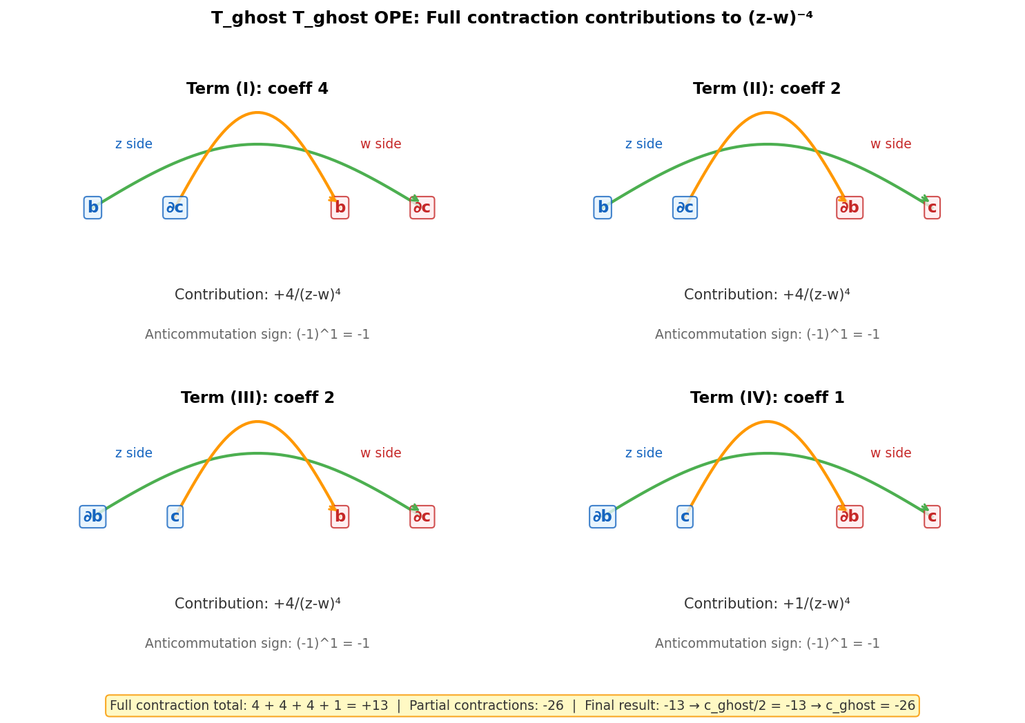
Fig. H.2: Full contraction patterns for the T_ghost T_ghost OPE. For each of the four terms, the possible contraction patterns between z-side and w-side fields are shown as arcs. The contributions to (z-w)⁻⁴ are determined from the anticommuting field rearrangement signs and the pole orders of each contraction.
Determining the Central Charge¶
🟡 Lina: Adding all 4 terms:
Summarizing the absolute values of the \((z-w)^{-4}\) coefficients for each term:
- Term (I): \(4\)
- Term (II): \(4\)
- Term (III): \(4\)
- Term (IV): \(1\)
Total \(4 + 4 + 4 + 1 = 13\).
🔵 Kai: \(4+4+4+1\)... adds up neatly to 13.
🟡 Lina: Regarding the overall sign: The final result is \(-13\). The physical reason the sign is negative is clear: a loop (closed propagation) of anticommuting fields always produces an overall \((-1)\) (same origin as the fermion loop sign rule in Quantum Field Theory Quantum Field Theory Ch. 12). The full contraction in the \(TT\) OPE corresponds to "ghost fields tracing a closed loop," and this \((-1)\) multiplies the whole thing. Rigorous sign tracking requires consistently applying additional sign rules for the relationship between radial ordering and normal ordering of anticommuting fields across all contraction patterns, which goes beyond this appendix. See Polchinski Vol.1 §2.5, §3.3 for the complete derivation.
What we confirmed in this appendix is where the number "\(13\)" comes from—the breakdown of absolute values of contributions from the four terms—which is uniquely determined by the pole orders and coefficients of each term's contractions.
In the calculation above, we showed only one contraction pattern for each term. Another pattern exists (e.g., for term (II): \(b(z) \leftrightarrow \partial b(w)\), \(\partial c(z) \leftrightarrow c(w)\)), but \(\langle b(z)\, \partial b(w)\rangle = \partial_w\langle b(z)\, b(w)\rangle = 0\) and \(\langle \partial c(z)\, c(w)\rangle = \partial_z\langle c(z)\, c(w)\rangle = 0\) (no propagator between same-type fields), so they all vanish. The same holds for terms (I) and (IV).
The above calculation confirms where the absolute value \(13 = 4 + 4 + 4 + 1\) of the \((z-w)^{-4}\) coefficient comes from. Complete determination of the overall sign requires rigorously tracking the sign rules in Wick's theorem between normal-ordered products of anticommuting fields (which depend on the ordering convention within normal-ordered products) and is insufficient with this appendix's simplified prescription. From the complete derivation (Polchinski Vol.1 §2.5, §3.3), the final result is:
Note that in the actual \(TT\) OPE, partial contractions (contracting only 2 of the 4 fields and leaving the remaining 2 as a normal-ordered product) also exist, but they do not contribute to \((z-w)^{-4}\). Let's verify why.
The highest pole obtainable from a partial contraction is \((z-w)^{-3}\) (e.g., \(\langle \partial c(z)\, \partial b(w)\rangle = -2/(z-w)^3\)). Taylor expanding the remaining normal-ordered field \(\phi(z)\) around \(w\) gives \(\phi(z) = \phi(w) + (z-w)\partial\phi(w) + \cdots\), but since the normal-ordered field carries only terms of order \((z-w)^0\) and higher, multiplying with \((z-w)^{-3}\) gives poles no higher than \((z-w)^{-3}\). It cannot reach \((z-w)^{-4}\).
⚪ Mei: So "you can't get \((z-w)^{-4}\) without contracting everything"—the central charge is determined by full contractions alone.
🟡 Lina: Let's verify with a concrete example. In term (I) \(4\, :\!b\partial c\!:(z)\, :\!b\partial c\!:(w)\), contracting only \(\partial c(z)\) with \(b(w)\) gives \(\langle \partial c(z)\, b(w)\rangle = -1/(z-w)^2\), leaving \(:\!b(z)\, \partial c(w)\!:\) as a normal-ordered product. Expanding \(b(z) = b(w) + (z-w)\partial b(w) + \cdots\), the whole thing has poles of \((z-w)^{-2}\) or lower. In term (II), contracting \(\partial c(z)\) with \(\partial b(w)\) gives \(-2/(z-w)^3\), but the Taylor expansion of the remaining \(b(z)\, c(w)\) starts at \((z-w)^0\), so the whole thing is \((z-w)^{-3}\) or lower. Neither reaches \((z-w)^{-4}\).
Partial contractions contribute to the \((z-w)^{-2}\) term (\(2T(w)/(z-w)^2\)) and the \((z-w)^{-1}\) term (\(\partial T(w)/(z-w)\)). The result is:
Comparing with the general form of the \(TT\) OPE (Ch. 16 16.5 "Energy-Momentum Tensor and Re-derivation of the Virasoro Algebra") \(T T \sim \frac{c/2}{(z-w)^4} + \cdots\):
🔵 Kai: I can see how \(-26\) comes out, but honestly I feel a bit uneasy. In the calculation we followed, we got \(+13\), and then we're told "with the correct sign rules it's \(-13\)"—without concretely seeing where the sign flips, it's hard to be fully convinced.
🟡 Lina: In this appendix we tracked signs using "hop counts when extracting fields from normal-ordered products," but actually there are additional sign rules in the relationship between radial ordering and normal ordering for anticommuting fields—\(\mathcal{R}[\psi(z)\chi(w)] = \langle \psi(z)\chi(w)\rangle + :\!\psi(z)\chi(w)\!:\), but swapping the field order gives \(\mathcal{R}[\chi(w)\psi(z)] = \langle \chi(w)\psi(z)\rangle - :\!\psi(z)\chi(w)\!:\) with a minus in front of the normal-ordered product. In Wick's theorem between normal-ordered products, the sign of the remaining normal-ordered product after contraction accumulates this effect. When you correctly track this across all contraction patterns, the total becomes \(-13\). See Polchinski Vol.1 §2.5, §3.3 for the complete derivation.
🔵 Kai: I see... the complete sign tracking is beyond this appendix's scope, but the physical reason that "fermion loops produce \((-1)\)" determining the sign makes sense to me. Since we could completely trace where the absolute value \(13\) (the breakdown \(4+4+4+1\)) comes from, I feel I've understood the core. But one thing I'm curious about—isn't \(4+4+4+1 = 13\) specific to \(\lambda = 2\)? How does the breakdown change for different \(\lambda\)?
🟡 Lina: Good question. For general \(\lambda\), the coefficients of each term become \(\lambda^2\), \(\lambda(1-\lambda)\), \((1-\lambda)\lambda\), \((1-\lambda)^2\), and the pole orders also change according to the distribution of derivatives. Adding everything up gives \(6\lambda^2 - 6\lambda + 1\)—this is exactly what's inside the general formula we'll see in the next section, H.7.
✅ Comprehension Check: When reading off the central charge from the \((z-w)^{-4}\) coefficient of the \(T_{\text{ghost}}\, T_{\text{ghost}}\) OPE, comparison with the general form \(TT \sim \frac{c/2}{(z-w)^4} + \cdots\) gives \(c_{\text{ghost}} = -26\). The \((z-w)^{-4}\) coefficient is \(-13\)—what operations produce this?
Answer
We expand the product of \(T_{\text{ghost}}(z) = -2:b\partial c: + :\partial b\, c:\) to get 4 terms, apply Wick's theorem for anticommuting fields to each, and enumerate all patterns contracting all fields (vacuum expectation values). Correctly tracking the signs from anticommuting field reordering and summing all terms gives the \((z-w)^{-4}\) coefficient as \(-13\).
Calculation note: To completely track the "rearrangement signs" in the above term-by-term calculation requires explicitly showing the anticommuting field reordering at each step. This appendix showed only the absolute value structure of each term and the consequence of the signs. For the complete derivation, see Polchinski String Theory Vol.1 §3.3 or Blumenhagen-Lüst-Theisen Basic Concepts of String Theory §3.3.3.
H.7 The General \(\lambda\) Case — The Formula \(c = -2(6\lambda^2 - 6\lambda + 1)\)¶
🟡 Lina: Performing the above calculation for general \(\lambda\) yields a central charge formula encompassing a broad family including the bosonic string's \(bc\) ghost system (\(\lambda = 2\)):
Checks:
- \(\lambda = 2\): \(c = -2(24 - 12 + 1) = -2 \cdot 13 = -26\) ✓ (string theory reparametrization ghosts)
- \(\lambda = 1/2\): \(c = -2(3/2 - 3 + 1) = -2 \cdot (-1/2) = 1\) (free fermion)
- \(\lambda = 3/2\): If a system with \(\lambda = 3/2\) were an anticommuting field (\(bc\) system), the formula would give \(c = -2(6\cdot\frac{9}{4} - 6\cdot\frac{3}{2} + 1) = -2(\frac{27}{2} - 9 + 1) = -2 \cdot \frac{11}{2} = -11\). However, the \(\beta\gamma\) ghosts of the superstring are actually commuting fields (bosonic), and the sign of the central charge is flipped.
🔵 Kai: Wait a moment. Why do the supersymmetry ghosts alone become commuting fields? In Section H.1 the story was "anticommuting fields are needed to produce the determinant."
🟡 Lina: Good question. Let's revisit the logic of Section H.1. In the Faddeev-Popov procedure, we "replace gauge parameters with fields." The core rule is:
- Gauge parameter is commuting (ordinary number) → make the ghost field anticommuting (to produce \(\det M\) via a Grassmann Gaussian integral)
- Gauge parameter is anticommuting (Grassmann odd) → make the ghost field commuting (to produce \((\det M)^{-1}\) via an ordinary Gaussian integral)
In other words, the general rule is "introduce a field with statistics opposite to that of the gauge parameter."
⚪ Mei: So the type of ghost field flips depending on the "character" of the gauge parameter.
🟡 Lina: The parameter of ordinary gauge symmetry (coordinate transformations \(\delta\sigma^a\)) is an ordinary number (commuting), so the ghost \(c\) becomes anticommuting. On the other hand, the gauge parameter of supersymmetry is already anticommuting (Grassmann odd)—supersymmetry is a transformation that exchanges bosons and fermions, and its parameter itself has fermionic character (see Ch. 17). Therefore the supersymmetric ghost is conversely a commuting (Grassmann even) field—the \(\beta\gamma\) system. The Gaussian integral for commuting fields gives \(\int \mathcal{D}\bar\beta\, \mathcal{D}\gamma\, e^{-\bar\beta M \gamma} = (\det M)^{-1}\), providing exactly the needed inverse.
⚪ Mei: So "whether you want to produce \(\det M\) or \((\det M)^{-1}\)" determines whether you use anticommuting or commuting fields.
🟡 Lina: Exactly. And the reason the sign of the central charge flips is also clear—the \(\beta\gamma\) system is a commuting field, so the fermion loop \((-1)\) doesn't appear. As a result, the sign of the \((z-w)^{-4}\) coefficient in the \(TT\) OPE is opposite to the \(bc\) system. Therefore:
🔵 Kai: Oh, the \(-11\) of the \(bc\) system just flips sign to \(+11\). That's clean.
⚪ Mei: So \(\lambda\) determines the conformal weight of the field, and the same OPE calculation structure uniquely produces the central charge—\(\lambda = 2\) for the bosonic string ghost, \(\lambda = 1/2\) for the free fermion, all covered by a single formula.
🔵 Kai: With \(\lambda = 1/2\) giving \(c = 1\), that's different from the free fermion single-component central charge \(c = 1/2\) from Ch. 16, right? Is it because the \(bc\) system has two fields \(b\) and \(c\) so it's doubled? But then for \(\lambda = 2\) the ghost also has two fields \(b\) and \(c\)—why don't we say "doubled" there?
🟡 Lina: Good question. The \(bc\) system with \(\lambda = 1/2\) corresponds to a "complex fermion" (\(b\) and \(c\) are two independent components), giving \(c = 1\). A single real fermion component has \(c = 1/2\), and two components (complex fermion) give \(c = 1\). For the \(\lambda = 2\) ghost it's the same—the central charge of the entire system combining both \(b\) and \(c\) fields is \(-26\). We don't say "\(-13\) per component." The formula \(c = -2(6\lambda^2 - 6\lambda + 1)\) gives the central charge of the entire \(bc\) system (including both fields) from the start.
In Ch. 17 (superstring theory), in addition to the \(bc\) ghost (\(\lambda = 2, c = -26\)), the superconformal symmetry ghost \(\beta\gamma\) system (\(\lambda = 3/2, c = +11\)) appears. From the condition that the sum of the matter field central charge (\(D\) bosons (each \(c = 1\)) + \(D\) real fermions (each \(c = 1/2\)) \(= D + D/2 = 3D/2\)) and ghosts equals zero:
The critical dimension \(D = 10\) of the superstring emerges from exactly the same logic as the bosonic string.
🔵 Kai: Both the bosonic string \(D=26\) and the superstring \(D=10\) come from the single condition "total central charge equals zero." That's unified.
✅ Comprehension Check: In the general \(\lambda\) central charge formula for the \(bc\) system \(c = -2(6\lambda^2 - 6\lambda + 1)\), setting \(\lambda = 1/2\) gives \(c = 1\). How many components of free fermions does this correspond to?
Answer
The \(bc\) system with \(\lambda = 1/2\) corresponds to a "complex fermion" (\(b\) and \(c\) are two independent components), giving \(c = 1\). The central charge of a single real fermion component is \(c = 1/2\), and two components (complex fermion) give \(c = 1\), which is consistent.
H.8 The BRST Charge and Selection of Physical States (Overview)¶
🟡 Lina: To eliminate the non-physical states introduced by ghost fields, a special global symmetry called BRST (Becchi-Rouet-Stora-Tyutin) symmetry is introduced. Specifically:
- BRST charge \(Q_B\): A particular combination involving ghost fields that satisfies \(Q_B^2 = 0\) (nilpotency)
- Physical states: States satisfying \(Q_B |\text{phys}\rangle = 0\), modulo the equivalence \(|\text{phys}\rangle \sim |\text{phys}\rangle + Q_B|\chi\rangle\) (BRST-exact forms)
🔵 Kai: \(Q_B^2 = 0\) means "acting twice makes it vanish," right? Why can that be used to select physical states?
🟡 Lina: \(Q_B^2 = 0\) guarantees that "states created by \(Q_B\)" are contained within "states annihilated by \(Q_B\)." Physical states are "annihilated by \(Q_B\) but not created by \(Q_B\)"—in mathematics, the structure of extracting such "closed but not exact" elements is called cohomology. Intuitively, it's like a "sieve that selects only essentially new states."
⚪ Mei: "Annihilated by \(Q_B\)" but "not created by \(Q_B\)"—those are the genuine physical states, as a selection criterion.
🟡 Lina: And when we impose \(Q_B^2 = 0\) in quantum theory, the condition:
automatically emerges. This is the origin of the critical dimension condition used in 16.7 "CFT Re-derivation of the Critical Dimension".
⚪ Mei: The ghost fields introduced for gauge fixing in turn become the tool for selecting physical states.
✅ Comprehension Check: What role does the nilpotency \(Q_B^2 = 0\) of the BRST charge \(Q_B\) play in the selection of physical states?
Answer
\(Q_B^2 = 0\) guarantees that "states created by \(Q_B\)" (\(Q_B|\chi\rangle\)) are contained within "states annihilated by \(Q_B\)" (\(Q_B|\text{phys}\rangle = 0\)). Physical states are defined as "annihilated by \(Q_B\) but not created by \(Q_B\)," forming a cohomological structure. Furthermore, requiring \(Q_B^2 = 0\) in quantum theory leads to \(c_{\text{matter}} + c_{\text{ghost}} = 0\), which determines the critical dimension.
🟡 Lina: For details, see Polchinski Vol.1 §4.2 or Kiritsis §3.11.
H.9 Summary¶
Table H.1: Summary of main results in Appendix H
| Item | Result |
|---|---|
| Action of the \(bc\) system | \(S = \frac{1}{2\pi}\int d^2z\, b\, \bar\partial c\) |
| Fundamental OPE | \(b(z)c(w) \sim 1/(z-w)\) |
| Energy-momentum tensor | \(T = -\lambda\, :b\,\partial c:+(1-\lambda)\, :\partial b\, c:\) (exchanging anticommuting fields within normal ordering changes the sign: \(:\partial b\, c: = -:c\,\partial b:\)) |
| Central charge (general formula) | \(c = -2(6\lambda^2 - 6\lambda + 1)\) |
| String theory ghost (\(\lambda=2\)) | \(c_{\text{ghost}} = -26\) |
| Superstring \(\beta\gamma\) system (commuting field, \(\lambda=3/2\)) | \(c_{\beta\gamma} = +11\) (sign flip from \(bc\) formula) |
| Critical dimension determination | \(c_{\text{matter}} + c_{\text{ghost}} = 0\) |
🟡 Lina: Now we can see where the \(c_{\text{ghost}} = -26\) "used as a result" in Ch. 16 16.7 "CFT Re-derivation of the Critical Dimension" comes from. Wick's theorem and OPE calculations for anticommuting fields are technical, but in principle they have the same structure as the bosonic field calculations in Ch. 16.
🔵 Kai: "Field statistics" and "distribution of derivatives" determine the central charge—it's technical, but ultimately it's just repeating the same OPE process.
⚪ Mei: From Faddeev-Popov all the way to \(c_{\text{ghost}} = -26\), connected by a single thread of logic—that feels satisfying.
References¶
- J. Polchinski, String Theory Vol.1, §3.2-3.3, §4.1-4.2
- R. Blumenhagen, D. Lüst, S. Theisen, Basic Concepts of String Theory, §3.3
- E. Kiritsis, String Theory in a Nutshell, §3.10-3.11
- M. Peskin, D. Schroeder, An Introduction to Quantum Field Theory, §16.2 (Implementation of Faddeev-Popov in non-Abelian gauge theories)
Feedback on this page
Let us know if something was unclear, incorrect, or could be improved.