Chapter 3: Classical Field Theory — Lagrangians and Noether's Theorem
Previously:
In Ch. 2, we reviewed the basic structure of special relativity. We confirmed Lorentz transformations, 4-vectors, the Minkowski metric \(\eta_{\mu\nu} = \mathrm{diag}(+1,-1,-1,-1)\), and the requirement that physical laws be Lorentz covariant. We also became familiar with natural units \(\hbar = c = 1\), the 4-derivative \(\partial_\mu\), and Einstein's summation convention.
Goals of This Chapter
- Introduce the field Lagrangian density \(\mathcal{L}(\phi, \partial_\mu\phi)\) and derive the field Euler-Lagrange equations from the principle of least action
- Prove Noether's theorem and confirm with concrete examples that "continuous symmetries imply conserved quantities" (spacetime translation → energy-momentum conservation, internal phase transformation → charge conservation)
- Finally, present the Lagrangians for the Klein-Gordon field, Dirac field, and Maxwell field, preparing for quantization in subsequent chapters
3.1 From Particle Mechanics to Field Mechanics
🟡 Lina: Now that we have the tools of special relativity from the previous chapter, today we'll develop the language of "field mechanics." You learned about the deep relationship between symmetries and conservation laws in Quantum Mechanics Ch. 26, right? Today we're extending that to the world of "fields."
🔵 Kai: In quantum mechanics we dealt with the particle wave function \(\psi(\mathbf{x}, t)\), but what's different about "field mechanics"?
🟡 Lina: Good question. In quantum mechanics, the particle positions \(q_i(t)\) were the dynamical variables. The degrees of freedom were finite—three for three dimensions. But a "field" is a quantity that has a value at every point in space. That means it has continuously infinite degrees of freedom. For example, something like a temperature distribution \(T(\mathbf{x}, t)\), where a single numerical value (a quantity with only magnitude and no direction) corresponds to each point in space, is called a "scalar field"—a field where a scalar (just a number) corresponds to each point. On the other hand, something like the electric field \(\mathbf{E}(\mathbf{x}, t)\), where a vector (a quantity with both magnitude and direction) corresponds to each point, is called a "vector field."
⚪ Mei: I see. So fields can be distinguished as scalar fields and vector fields. Temperature is a scalar field, the electric field is a vector field.
🟡 Lina: Exactly. Let me summarize the correspondence between particle mechanics and field theory in a table.
Table 3.1: Basic correspondence between particle mechanics and field theory
| Particle Mechanics | Field Theory | |
|---|---|---|
| Dynamical variables | \(q_1(t), q_2(t), \ldots, q_N(t)\) | \(\phi_a(\mathbf{x}, t)\) |
| Number of degrees of freedom | Finite (\(N\)) | Continuously infinite |
| Labels | Discrete index \(i = 1, \ldots, N\) | Continuous spatial coordinate \(\mathbf{x}\) and discrete \(a\) |
🔵 Kai: Since there's one degree of freedom at each point in space, you get infinitely many. Is it like each point on a rubber sheet being able to vibrate up and down independently? But "infinitely many degrees of freedom" sounds scary—won't the calculations break down?
🟡 Lina: That's a good concern. In fact, dealing with infinitely many degrees of freedom does lead to "divergence" problems later on—we'll tackle those head-on from Ch. 8 onward. But for now we're fine. The strength of the Lagrangian framework is that it works the same way whether there are finitely many or infinitely many degrees of freedom. As an image, particle mechanics is like tracking the motion of a "marble" sitting on a sheet. Field theory describes the vibrations of the sheet itself. Look at Fig. 3.1 "Limit from discrete system to continuous field"—it illustrates the limit from a discrete spring-mass system to a continuous field.
✅ Comprehension Check: How does the number of degrees of freedom of the dynamical variables differ between particle mechanics and field theory?
Answer
In particle mechanics, the degrees of freedom of the dynamical variables \(q_i(t)\) are finite (\(N\)), but in field theory, since the field \(\phi(\mathbf{x}, t)\) has a value at each point in space, the degrees of freedom are continuously infinite. The discrete index \(i\) is replaced by the continuous spatial coordinate \(\mathbf{x}\).
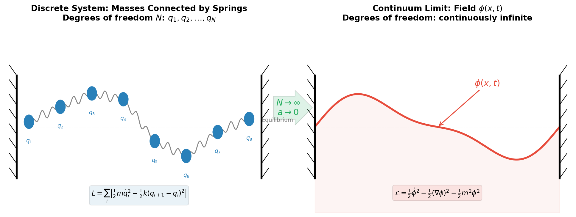
Fig. 3.1: Limit from discrete system to continuous field. From a discrete system (masses connected by springs, \(N\) degrees of freedom) to a continuous field \(\phi(x, t)\) (continuously infinite degrees of freedom). This shows how the discrete index \(i\) is replaced by the continuous coordinate \(x\).
Introduction of the Lagrangian Density
🟡 Lina: In particle mechanics, we defined the Lagrangian \(L(q, \dot{q}) = T - V\) and derived the equations of motion by minimizing (more precisely, making stationary) the action \(S = \int dt \, L\). We use exactly the same idea in field theory.
First, the Lagrangian in field theory is written as:
Here the index \(a\) is a label that distinguishes the type (component) of the field. For example, if there's only one scalar field, \(a\) takes only one value and can be omitted. If there are multiple real scalar fields \(\phi_1, \phi_2, \ldots\), we number them as \(a = 1, 2, \ldots\). For a field like the electromagnetic potential \(A_\mu\) with 4 components, formally \(a\) takes 4 values—however, in this case \(a\) is tied to spacetime directions (Lorentz indices), so the components mix under Lorentz transformations, which is different in character from being just a "number." For now, just remember that "\(a\) is a label distinguishing field components." We'll revisit this distinction when we treat the Maxwell field in detail.
🔵 Kai: What is \(\mathcal{L}\)? Is it different from \(L\)?
🟡 Lina: \(\mathcal{L}\) is called the Lagrangian density, meaning "Lagrangian per unit volume." It's the same idea as mass density \(\rho\) being "mass per unit volume." When you integrate over all of space, you get the total Lagrangian \(L\).
⚪ Mei: So the relationship between \(L\) and \(\mathcal{L}\) has the same structure as the relationship between mass \(M\) and mass density \(\rho\): \(M = \int d^3x \, \rho\).
🟡 Lina: Right. However, physicists are lazy, so they often just call \(\mathcal{L}\) the "Lagrangian" too. Judge from context.
And the action \(S\) is the integral of the Lagrangian density over all of 4-dimensional spacetime:
Here \(d^4x = dt \, d^3x\) is the 4-dimensional volume element.
🔵 Kai: Does \(\mathcal{L}\) depend only on \(\phi_a\) and \(\partial_\mu \phi_a\)? Don't second derivatives \(\partial_\mu \partial_\nu \phi\) enter?
🟡 Lina: Sharp question. Here we assume that \(\mathcal{L}\) depends only on the field and its first derivatives. This is the same spirit as \(L(q, \dot{q})\) not depending on \(\ddot{q}\) in particle mechanics. If you include second or higher derivatives, a problem called the Ostrogradsky instability arises, where the energy becomes unbounded from below—meaning the system can fall to arbitrarily low energy states, so no stable "ground state" exists. It's like a ball falling forever into a bottomless pit—physically it breaks down.
✅ Comprehension Check: What is the physical reason why the Lagrangian density must not depend on second or higher derivatives of the field?
Answer
A Lagrangian containing second or higher derivatives leads to Ostrogradsky instability, where the energy becomes unbounded from below (arbitrarily low energy states exist). This means the theory is physically unstable, so we assume \(\mathcal{L}\) depends only on the field and its first derivatives.
⚪ Mei: Summarizing the correspondence with particle mechanics:
Table 3.2: Lagrangian and action: particle vs. field comparison
| Particle Mechanics | Field Theory | |
|---|---|---|
| Lagrangian | \(L(q, \dot{q})\) | \(L = \int d^3x \, \mathcal{L}(\phi, \partial_\mu \phi)\) |
| Action | \(S = \int dt \, L\) | \(S = \int d^4x \, \mathcal{L}\) |
| Derivative dependence | Up to \(\dot{q}\) (first order) | Up to \(\partial_\mu \phi\) (first order) |
🟡 Lina: Perfect summary. One more important thing: in quantum field theory, the basic strategy is to construct the Lagrangian density \(\mathcal{L}\) as a Lorentz scalar (a quantity whose value doesn't change under Lorentz transformations). This ensures that the same form of the theory is obtained in any inertial frame. This is how we satisfy the requirement of Lorentz invariance that we learned in Ch. 2.
✅ Comprehension Check: Explain the relationship between the Lagrangian density \(\mathcal{L}\) and the Lagrangian \(L\) using the analogy of mass density.
Answer
Just as integrating the mass density \(\rho\) over all space gives the total mass \(M = \int d^3x\,\rho\), integrating the Lagrangian density \(\mathcal{L}\) over all space gives the Lagrangian \(L = \int d^3x\,\mathcal{L}\). \(\mathcal{L}\) is the "Lagrangian per unit volume."
3.2 The Principle of Least Action and the Field Euler-Lagrange Equations
🟡 Lina: In particle mechanics, the path \(q(t)\) that makes the action \(S\) stationary is the physically realized motion. We use exactly the same idea in field theory. We make a small deformation of the field configuration \(\phi_a(x)\) and require \(\delta S = 0\). I've drawn the variations for particle mechanics and field theory side by side in Fig. 3.2 "Image of the variational principle: particle mechanics (left) and field theory (right)", so compare them.
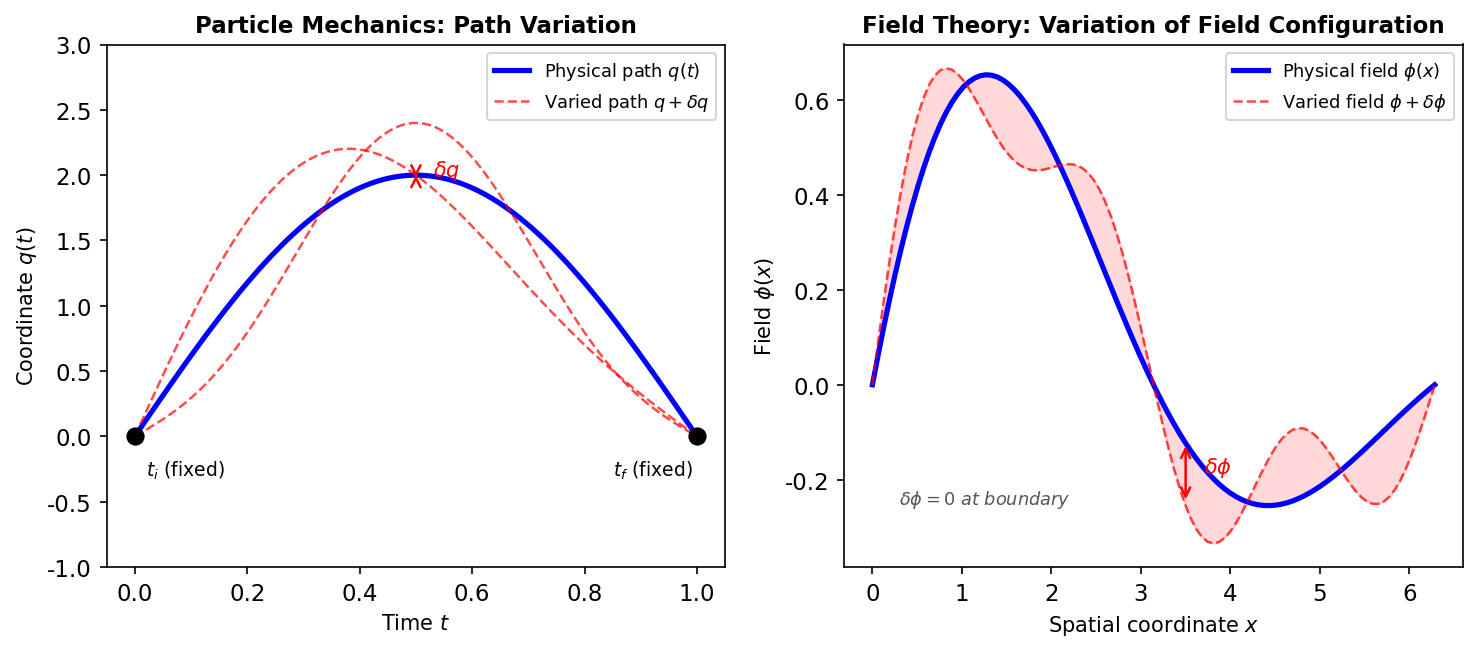
Fig. 3.2: Image of the variational principle: particle mechanics (left) and field theory (right). In particle mechanics, the path \(q(t)\) is deformed slightly with endpoints fixed. In field theory, the field configuration \(\phi(x)\) is deformed slightly with \(\delta\phi = 0\) at the spacetime boundary. In both cases, requiring \(\delta S = 0\) yields the equations of motion.
🔵 Kai: What does "deforming the field slightly" mean concretely?
🟡 Lina: We shift the field \(\phi_a(x)\) to \(\phi_a(x) + \delta\phi_a(x)\) by a small amount. However, at the spacetime boundary (infinity or initial/final times) we set \(\delta\phi_a = 0\). That is, we keep the endpoints fixed and only change the shape in between.
Now let's proceed with the derivation. The variation of the action is:
⚪ Mei: This is the formula for the total differential of a multivariable function. Since \(\mathcal{L}\) depends on "two variables" \(\phi_a\) and \(\partial_\mu \phi_a\), we're adding up the contributions from changes in each.
🔵 Kai: Wait a moment. \(\partial_\mu\phi\) can be computed from \(\phi\), so why can we treat it as an "independent variable"?
🟡 Lina: Good question. This is the same idea as when computing partial derivatives of \(L(q, \dot{q})\) in particle mechanics. \(\dot{q}\) is the time derivative of \(q(t)\) so it's determined by \(q\), but when computing the partial derivative \(\frac{\partial L}{\partial q}\), the convention is to "hold \(\dot{q}\) fixed and vary only \(q\)." Similarly, when computing \(\frac{\partial\mathcal{L}}{\partial\phi_a}\), we "hold \(\partial_\mu\phi_a\) fixed and vary only \(\phi_a\)." This is a procedural convention for the calculation, and after substituting into the Euler-Lagrange equation, the relationship between \(\partial_\mu\phi\) and \(\phi\) is properly restored, so don't worry.
🟡 Lina: That's right. The important thing here is that the order of the variation \(\delta\) and the derivative \(\partial_\mu\) can be exchanged:
This means "taking the small change then differentiating" gives the same result as "differentiating then taking the small change."
🔵 Kai: I see, \(\delta\) is the "shift slightly" operation and \(\partial_\mu\) is the "differentiate" operation, so it doesn't matter which you do first.
🟡 Lina: Right. Now we apply integration by parts to the second term of equation (3.3). This is the 4-dimensional version of the one-variable integration by parts \(\int u \, dv = uv - \int v \, du\).
The idea is this. Using the product rule (Leibniz rule) \(\partial_\mu(fg) = (\partial_\mu f)g + f(\partial_\mu g)\), we rearrange to get \(f(\partial_\mu g) = \partial_\mu(fg) - (\partial_\mu f)g\). Setting \(f = \frac{\partial\mathcal{L}}{\partial(\partial_\mu\phi_a)}\) and \(g = \delta\phi_a\):
🔵 Kai: What's the last term?
🟡 Lina: The last term is a total divergence. Recall the one-variable case: \(\int_a^b \frac{d}{dx}[f(x)]\,dx = f(b) - f(a)\), where the integral of a total derivative is determined only by the endpoint values. The same thing happens in 4 dimensions. Using the 4-dimensional Gauss's theorem (divergence theorem), \(\int d^4x\,\partial_\mu(\cdots)\) can be converted to a surface integral on the "boundary" of spacetime. And since we set \(\delta\phi_a = 0\) at the boundary, this term vanishes.
Therefore:
🔵 Kai: Since \(\delta S = 0\), this entire integral must be zero. But since \(\delta\phi_a\) is arbitrary... does that mean the contents of the square brackets themselves must be zero?
🟡 Lina: Exactly! If the contents of the brackets were nonzero at some point, we could choose a variation \(\delta\phi_a \neq 0\) only around that point, making \(\delta S \neq 0\)—contradicting "\(\delta S = 0\) for arbitrary \(\delta\phi_a\)." So the contents of the brackets must be zero at each point. This gives us the field Euler-Lagrange equations:
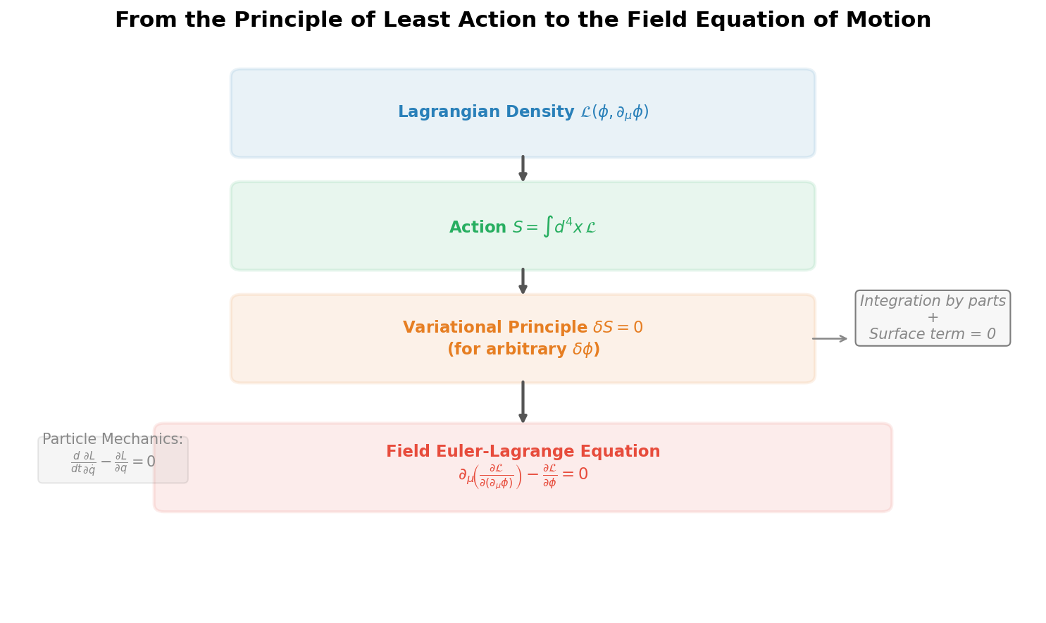
Fig. 3.3: Derivation of the equations of motion from the principle of least action. The flow of derivation: Lagrangian density → action → variational principle → Euler-Lagrange equations. Integration by parts and the vanishing of surface terms are the key steps.
🔵 Kai: Oh! This looks just like the particle mechanics Euler-Lagrange equation \(\frac{d}{dt}\frac{\partial L}{\partial \dot{q}} - \frac{\partial L}{\partial q} = 0\)!
🟡 Lina: It's exactly the natural extension. Let me summarize the correspondence:
Table 3.3: Euler-Lagrange equation: particle vs. field correspondence
| Particle Mechanics | Field Theory |
|---|---|
| \(\dfrac{d}{dt}\) | \(\partial_\mu\) (time derivative → spacetime derivative) |
| \(\dfrac{\partial L}{\partial \dot{q}}\) | \(\dfrac{\partial \mathcal{L}}{\partial(\partial_\mu \phi_a)}\) |
| \(\dfrac{\partial L}{\partial q}\) | \(\dfrac{\partial \mathcal{L}}{\partial \phi_a}\) |
⚪ Mei: The time derivative \(d/dt\) is replaced by the 4-dimensional derivative \(\partial_\mu\), and by summing over \(\mu\) (Einstein summation convention), it includes derivatives in both the time and space directions.
✅ Comprehension Check: In the derivation of the field Euler-Lagrange equations, why does the "surface term" that appears after integration by parts vanish?
Answer
Because we impose the boundary condition that the field variation \(\delta\phi_a\) is zero at the spacetime boundary (at infinity or at initial/final times), the term converted to a surface integral by Gauss's theorem vanishes.
Concrete Example: Derivation of the Klein-Gordon Equation
🟡 Lina: Let's use the Euler-Lagrange equation right away. Consider the following Lagrangian density for a real scalar field \(\phi(x)\):
🔵 Kai: Where does this Lagrangian come from? Why this particular form?
🟡 Lina: Very good question. There are three reasons for choosing this Lagrangian:
- It is a Lorentz scalar: \(\partial_\mu \phi \, \partial^\mu \phi\) doesn't change value under Lorentz transformations
- It contains only the field and its first derivatives: No second or higher derivatives
- It is the simplest: The simplest combination of Lorentz scalars that can be formed from \(\phi\) and \(\partial_\mu\phi\)
Let's look at the structure. Expanding using the metric tensor \(\eta^{\mu\nu} = \mathrm{diag}(+1,-1,-1,-1)\) that we learned in Ch. 2:
So:
🔵 Kai: Ah, when you expand it, you can see the \(T - V\) structure. \(\dot{\phi}^2\) is kinetic energy-like, and the rest is potential-like.
🟡 Lina: Exactly. Let's compare with particle mechanics' \(L = T - V\). \(\frac{1}{2}\dot{\phi}^2\) is the "kinetic energy-like term" related to the time variation of the field, while \(\frac{1}{2}(\nabla\phi)^2 + \frac{1}{2}m^2\phi^2\) are "potential energy-like terms" related to the spatial variation and the field value itself.
⚪ Mei: I see, the \(T - V\) structure of particle mechanics extends directly to fields.
🟡 Lina: Right. Now let's compute the partial derivatives needed for the Euler-Lagrange equation.
Step 1: Partial derivative with respect to \(\phi\)
The only term in \(\mathcal{L}\) containing \(\phi\) itself (without derivatives) is \(-\frac{1}{2}m^2\phi^2\). So:
Step 2: Partial derivative with respect to \(\partial_\mu \phi\)
We differentiate \(\mathcal{L} = \frac{1}{2}\eta^{\alpha\beta}\partial_\alpha\phi \, \partial_\beta\phi - \frac{1}{2}m^2\phi^2\) with respect to \(\partial_\mu\phi\). This works the same way as \(\frac{d}{dv}\left(\frac{1}{2}v^2\right) = v\):
🔵 Kai: Why does the index go up?
🟡 Lina: When you differentiate \(\frac{1}{2}\eta^{\alpha\beta}\partial_\alpha\phi \, \partial_\beta\phi\) with respect to \(\partial_\mu\phi\), the metric tensor raises the index. Writing it explicitly:
Let me supplement the intermediate calculation. Here \(\delta^\mu_\alpha\) is the Kronecker delta—equal to 1 when \(\mu = \alpha\), and 0 otherwise. The idea of differentiating \(\partial_\beta\phi\) with respect to \(\partial_\mu\phi\) works like this: think of \(\partial_0\phi, \partial_1\phi, \partial_2\phi, \partial_3\phi\) as 4 independent variables. For example, if you have 4 variables \(x, y, z, w\), then \(\frac{\partial y}{\partial x} = 0\) and \(\frac{\partial y}{\partial y} = 1\), right? Similarly, \(\frac{\partial(\partial_\beta\phi)}{\partial(\partial_\mu\phi)}\) is "1 only when \(\beta = \mu\), and 0 otherwise"—that is, \(\delta^\mu_{\;\beta}\).
⚪ Mei: So the metric tensor raises the remaining index through the Kronecker delta—that's the mechanism.
🟡 Lina: Exactly. The reason \(\delta^\mu_{\;\beta}\) has \(\mu\) as a superscript is to be consistent with the "index raising operation" learned in Ch. 2. Let's look at it concretely. In the first term, \(\delta^\mu_\alpha\) selects \(\alpha = \mu\), giving \(\eta^{\alpha\beta} \to \eta^{\mu\beta}\), and then \(\eta^{\mu\beta}\partial_\beta\phi = \partial^\mu\phi\) (this is the "raising the index with the metric" operation). The second term similarly has \(\delta^\mu_\beta\) selecting \(\beta = \mu\), giving \(\eta^{\alpha\mu}\partial_\alpha\phi = \partial^\mu\phi\). The two terms give the same \(\partial^\mu\phi\) thanks to the symmetry of the metric tensor \(\eta^{\alpha\beta} = \eta^{\beta\alpha}\).
In short, differentiating with \(\frac{\partial}{\partial(\partial_\mu\phi)}\) causes the metric tensor to lift the remaining index up, giving the result \(\partial^\mu\phi\) (with an upper index). For now, just keep in mind that "this calculation rule produces \(\partial^\mu\phi\)."
Step 3: Substituting into the Euler-Lagrange equation
Substituting into equation (3.7):
🔵 Kai: This is the Klein-Gordon equation we saw in Quantum Mechanics Ch. 27!
🟡 Lina: Exactly! In Quantum Mechanics Ch. 27, we started from the relativistic energy-momentum relation \(E^2 = |\mathbf{p}|^2 + m^2\) and derived it by "replacing with operators." This time it was derived automatically from the Lagrangian. Let me write it in a more familiar form. Since \(\partial_\mu\partial^\mu = \frac{\partial^2}{\partial t^2} - \nabla^2\):
This \(\partial_\mu\partial^\mu\) is written collectively as \(\Box\) and called the d'Alembertian. Using this, the Klein-Gordon equation can be written compactly as \((\Box + m^2)\phi = 0\). And if we set \(m = 0\), we get \(\Box\phi = 0\)—the ordinary wave equation.
Reading Off the Dispersion Relation
🟡 Lina: Let's try a plane wave solution to the Klein-Gordon equation. We assume the form \(\phi \propto e^{-iEt + i\mathbf{p}\cdot\mathbf{x}}\). Here \(E\) and \(\mathbf{p}\) are as yet unknown constant parameters—we'll find out what they correspond to by substituting into the equation.
Substituting:
If \(\phi \neq 0\):
🔵 Kai: That's Einstein's energy-momentum relation itself! Including the \(m^2\phi^2\) term in the Lagrangian corresponds to giving the particle mass \(m\).
🟡 Lina: Exactly. If \(m = 0\) then \(E = |\mathbf{p}|\), which is the dispersion relation for a massless particle like the photon. If \(m \neq 0\), then even at \(|\mathbf{p}| = 0\) we have \(E = m \neq 0\)—a rest energy \(E = mc^2\) (which is \(E = m\) in natural units) exists.
✅ Comprehension Check: Write the equation of motion derived from the Lagrangian density \(\mathcal{L} = \frac{1}{2}\partial_\mu\phi\,\partial^\mu\phi\) (without the \(m^2\) term), and its dispersion relation.
Answer
The equation of motion is \(\partial_\mu\partial^\mu\phi = 0\) (the wave equation). The dispersion relation is \(E^2 = |\mathbf{p}|^2\), i.e., \(E = |\mathbf{p}|\). This corresponds to a massless particle.
3.3 Noether's Theorem — Deriving Conservation Laws from Symmetries
🟡 Lina: Now we come to the heart of this chapter. In Quantum Mechanics Ch. 26, you learned that "if there's a symmetry, there's a conserved quantity." The specific correspondences we saw were:
Table 3.4: Correspondence between symmetries and conserved quantities
| Symmetry | Conserved Quantity |
|---|---|
| Spatial translation invariance | Momentum |
| Rotational invariance | Angular momentum |
| Time translation invariance | Energy |
Today we'll mathematically prove this relationship in the context of field theory. This is Noether's theorem.
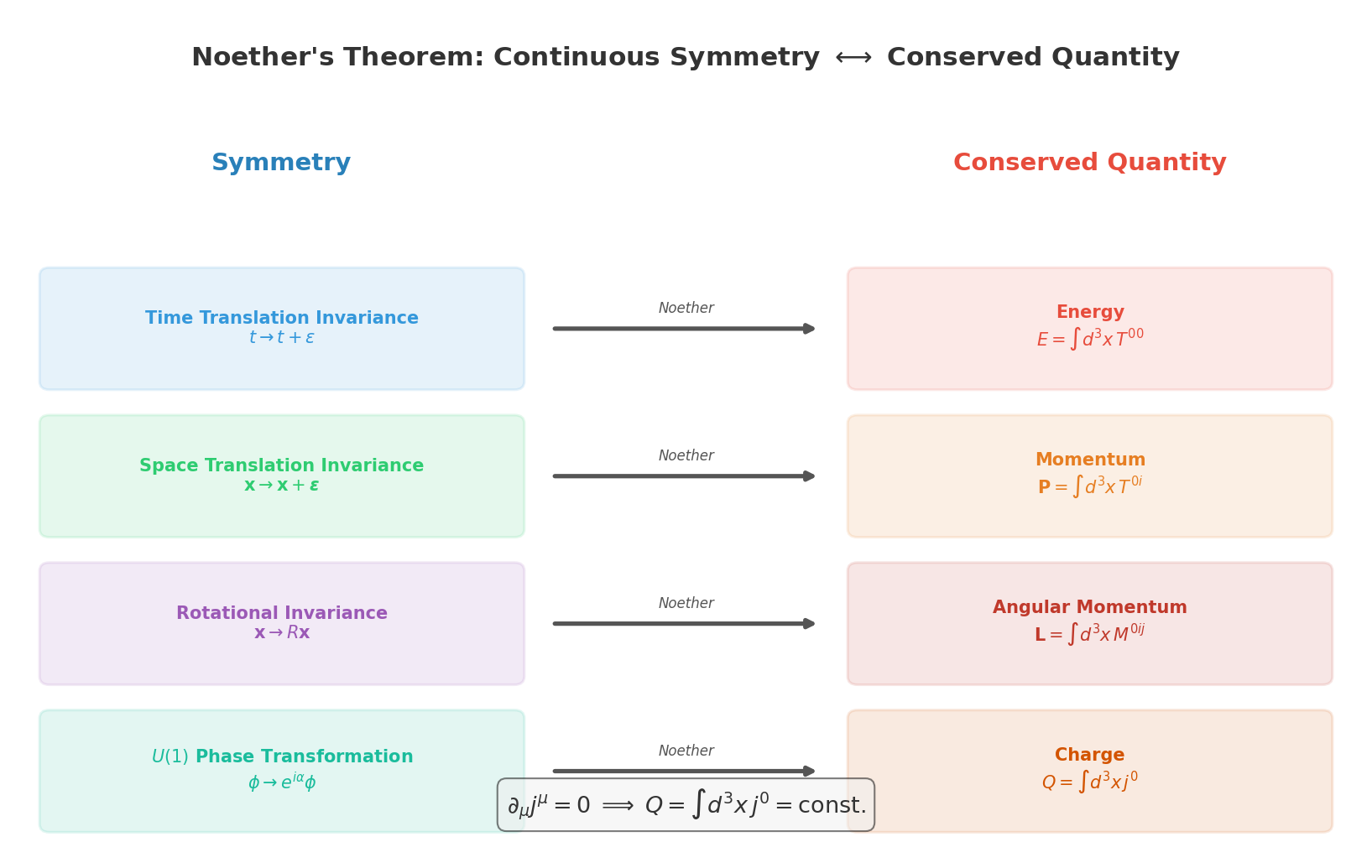
Fig. 3.4: Correspondence between symmetries and conserved quantities via Noether's theorem — spacetime translation → energy-momentum, rotation → angular momentum, \(U(1)\) phase transformation → charge (\(U(1)\) will be treated in detail later in this chapter).
🔵 Kai: This is the theorem proved by Emmy Noether, right?
🟡 Lina: Yes. Published in 1918, it's said to be one of the most beautiful and most practical theorems in physics. I've illustrated the correspondence between symmetries and conserved quantities in Fig. 3.4 "Correspondence between symmetries and conserved quantities via Noether's theorem", so keep the big picture in mind as we go. Let me state the theorem first:
Noether's Theorem: If the Lagrangian density \(\mathcal{L}\) is invariant under a certain continuous transformation, then there exists a corresponding conserved current \(j^\mu\) satisfying \(\partial_\mu j^\mu = 0\).
🔵 Kai: What is a "conserved current"? "Current" means electric current, right? Why does a current come from a symmetry?
🟡 Lina: You'll understand if we write out the equation \(\partial_\mu j^\mu = 0\) in components:
🔵 Kai: Ah, this is the continuity equation! It's the same form as when charge density \(\rho\) and current density \(\mathbf{j}\) satisfy \(\frac{\partial \rho}{\partial t} + \nabla \cdot \mathbf{j} = 0\) in electromagnetism.
🟡 Lina: Exactly. \(j^0\) can be interpreted as "a density of something," and \(\mathbf{j} = (j^1, j^2, j^3)\) as "a flow of something." And the quantity obtained by integrating \(j^0\) over all space:
does not change in time—it's a conserved quantity.
🔵 Kai: \(Q\) being conserved means \(\frac{dQ}{dt} = 0\), right? But if I take the time derivative of \(Q = \int d^3x\,j^0\), I get \(\frac{dQ}{dt} = \int d^3x\,\frac{\partial j^0}{\partial t}\), and I don't yet see why this is zero.
🟡 Lina: Substituting the continuity equation \(\frac{\partial j^0}{\partial t} = -\nabla\cdot\mathbf{j}\) gives \(\frac{dQ}{dt} = -\int d^3x\,\nabla\cdot\mathbf{j}\). Using Gauss's theorem, this can be converted to a surface integral. \(\int d^3x\,\nabla\cdot\mathbf{j}\) equals the surface integral of \(\mathbf{j}\) over a sufficiently large sphere, right? Here we use a physical boundary condition. In field theory, we impose the condition that "the total energy of the system is finite." Intuitively, if the field \(\phi\) doesn't approach zero at infinity, the energy density \(T^{00} \sim \phi^2\) would extend everywhere in space, and integrating over all space would give infinity—physically impossible. So the condition of "finite energy" requires that the field \(\phi\) and its derivatives approach zero sufficiently fast at infinity. Then since \(j^\mu\) is also constructed from \(\phi\) and its derivatives, it decays at infinity. Therefore, taking the sphere sufficiently large makes the surface integral zero, showing \(\frac{dQ}{dt} = 0\).
⚪ Mei: So the logical flow is "physically finite-energy field" → "field decays at infinity" → "surface integral is zero" → "\(Q\) is conserved."
Proof of Noether's Theorem
🟡 Lina: Now let's enter the proof. Suppose the field \(\phi(x)\) undergoes a small continuous transformation:
The variation of the Lagrangian density is:
🔵 Kai: This has the same form as equation (3.3).
🟡 Lina: Right. Now we use a manipulation trick. First, use \(\delta(\partial_\mu\phi) = \partial_\mu(\delta\phi)\). Next, using the product rule (Leibniz rule) \(\partial_\mu(fg) = (\partial_\mu f)g + f(\partial_\mu g)\) rearranged as \(f(\partial_\mu g) = \partial_\mu(fg) - (\partial_\mu f)g\), we rewrite the second term:
⚪ Mei: I see, it's just rearranging the product rule we learned in high school.
🟡 Lina: Exactly. Substituting equation (3.18) into equation (3.17):
🔵 Kai: The contents of the first square bracket are... ah! That's the left-hand side of the Euler-Lagrange equation!
🟡 Lina: Yes! This is the key point of Noether's theorem. Let me clarify what's different between before and now.
- Deriving the Euler-Lagrange equation (what we did earlier): \(\phi(x)\) was still an arbitrary unknown field. We required "\(\delta S = 0\) for arbitrary \(\delta\phi\)." Since \(\delta\phi\) can be anything, the integrand itself must be zero—this is how the equation of motion was derived.
- Noether's theorem (what we're doing now): \(\phi(x)\) already satisfies the equation of motion—it's a physically realized field configuration. On top of that, we're applying a specific transformation (symmetry transformation) \(\delta\phi\).
⚪ Mei: Even though we're using the same equation (3.19), the premises are completely different. Before it was "we considered arbitrary \(\delta\phi\) to derive the equation," now it's "we're considering a specific \(\delta\phi\) on a field that satisfies the equation."
🟡 Lina: Exactly. On a field where the equation of motion holds, the contents of the square bracket (= left-hand side of the Euler-Lagrange equation) are identically zero regardless of what \(\delta\phi\) is—because the contents of the bracket are a quantity written only in terms of \(\phi\) and its derivatives (independent of \(\delta\phi\)), and that quantity is zero by the equation of motion. Therefore:
Now we use the symmetry condition. "\(\mathcal{L}\) is invariant under this transformation" means \(\delta\mathcal{L} = 0\). Therefore:
🔵 Kai: Wow, is that all it takes to get a conservation law! The contents of the parentheses directly become the conserved current.
🟡 Lina: So if we name the contents of the parentheses \(j^\mu\): \(j^\mu \equiv \frac{\partial \mathcal{L}}{\partial(\partial_\mu \phi)} \, \delta\phi\) satisfies \(\partial_\mu j^\mu = 0\)—this is the conserved current.
⚪ Mei: Just combining the symmetry condition \(\delta\mathcal{L} = 0\) and the equation of motion automatically produces a conservation law.
🟡 Lina: Precisely. Now, it's convenient to decompose the infinitesimal transformation into "magnitude" and "direction." For example, for a phase transformation \(\delta\phi = i\alpha\,\phi\), \(\alpha\) represents "how much to rotate" (the magnitude) and \(i\phi\) represents "in which direction the change occurs" (the pattern). In general, we write \(\delta\phi = \epsilon \, D\phi\). \(\epsilon\) is a small constant parameter representing "how much to transform," and \(D\phi\) is "what remains after factoring out \(\epsilon\)"—it represents "how the field changes in form."
🔵 Kai: Is \(D\) related to the differential \(d\)?
🟡 Lina: Good question. The \(D\) here is not a differential operator but simply a symbol representing "what remains of \(\delta\phi\) after factoring out the constant parameter \(\epsilon\)." That is, from the defining decomposition \(\delta\phi = \epsilon \times D\phi\), we get \(D\phi \equiv \delta\phi / \epsilon\).
Checking with the phase transformation example: \(\delta\phi = i\alpha\,\phi\), so \(\epsilon = \alpha\) and \(D\phi = \delta\phi/\epsilon = i\phi\). So \(D\phi\) is "the field value multiplied by \(i\)"—just the field value times a constant. The form of \(D\phi\) changes with different types of transformations. When we treat spacetime translations in the next section, a different form \(D\phi = \partial_\nu\phi\) will appear, so we'll confirm it again there.
The reason we bother separating into \(\epsilon\) and \(D\phi\) is that in equation (3.21), \(\partial_\mu\!\left(\frac{\partial \mathcal{L}}{\partial(\partial_\mu \phi)} \cdot \epsilon\,D\phi\right) = 0\), and since \(\epsilon\) is a constant, it can be pulled outside \(\partial_\mu\). Dividing both sides by \(\epsilon \neq 0\), the expression for the conserved current becomes a universal form independent of the value of \(\epsilon\)—meaning the conserved quantity is determined only by the type of symmetry, regardless of "how much we transformed."
Written this way, replacing \(\delta\phi\) with \(\epsilon\,D\phi\) in equation (3.21) gives \(\partial_\mu\!\left(\frac{\partial \mathcal{L}}{\partial(\partial_\mu \phi)} \cdot \epsilon\,D\phi\right) = 0\). Since \(\epsilon\) doesn't depend on \(x\), it can be pulled outside \(\partial_\mu\):
Dividing both sides by \(\epsilon \neq 0\), we can define the conserved current \(j^\mu\) as:
This is the conclusion of Noether's theorem (for the case \(\delta\mathcal{L} = 0\)).
Note: Equation (3.22) is directly usable when \(\delta\mathcal{L} = 0\) (the Lagrangian density is completely invariant) and the transformation parameter is a single constant. The \(U(1)\) phase transformation treated in the next section (\(\delta\phi = i\alpha\,\phi\), with single parameter \(\alpha\) and \(\delta\mathcal{L} = 0\)) is exactly this case. On the other hand, for spacetime translations, \(\delta\mathcal{L} \neq 0\) (though it becomes a total derivative) and the parameter has 4 components, so we need the generalization in equation (3.25) derived in the next "Generalization: When \(\delta\mathcal{L}\) is a Total Derivative"—we'll see it concretely there, so for now just remember that "equation (3.22) is the basic form for the case \(\delta\mathcal{L} = 0\)."
The generalization to the case where \(\delta\mathcal{L} \neq 0\) but is a total derivative will be treated immediately after in "Generalization: When \(\delta\mathcal{L}\) is a Total Derivative".
🔵 Kai: Amazing... just combining symmetry (\(\delta\mathcal{L} = 0\)) and the equation of motion (Euler-Lagrange equation) produces a conserved current.
🟡 Lina: The beauty of this proof is that two independent conditions—"symmetry" and "equation of motion"—converge into a single conclusion: a conservation law.
Generalization: When \(\delta\mathcal{L}\) is a Total Derivative
🟡 Lina: Actually, Noether's theorem can be used even when \(\delta\mathcal{L} \neq 0\). When we consider spacetime translations in the next section, the Lagrangian density itself changes (\(\delta\mathcal{L} \neq 0\)), but if the change has a special form, we can still derive a conservation law—this situation actually arises.
Specifically, it's sufficient if \(\delta\mathcal{L}\) takes the form of a 4-dimensional divergence (total derivative):
🔵 Kai: Can we still call it a "symmetry" if \(\delta\mathcal{L} \neq 0\)?
🟡 Lina: Good question. The point is "whether the action \(S\) changes." Converting \(\delta S = \int d^4x\,\delta\mathcal{L} = \int d^4x\,\partial_\mu K^\mu\) using Gauss's theorem gives a surface integral on the spacetime boundary. As an analogy with a one-variable integral, \(\int_a^b \frac{df}{dx}dx = f(b) - f(a)\)—the integral of a total derivative is determined only by the endpoint values, right? The same thing happens in 4 dimensions. Under the condition that we fix the field at the boundary (\(\delta\phi = 0\)), this surface term doesn't contribute to the derivation of the equation of motion. So if \(\delta\mathcal{L}\) is a total derivative, even though the Lagrangian density value changes, the physics (equations of motion) doesn't change. This is sometimes called a quasi-symmetry, but you don't need to remember the name. What matters is that "if \(\delta\mathcal{L}\) is a total derivative, Noether's theorem applies."
⚪ Mei: I see. \(\delta\mathcal{L} = 0\) means "the density doesn't change," and \(\delta\mathcal{L} = \partial_\mu K^\mu\) means "the density changes but the action (the total integral) doesn't change"—both are physically equivalent.
🟡 Lina: In this case, the left side of equation (3.20) and the right side of equation (3.23) are both equal to \(\delta\mathcal{L}\):
Taking the difference of both sides and factoring out \(\partial_\mu\):
So the conserved current is:
⚪ Mei: For spacetime translations, \(\delta\mathcal{L} \neq 0\) but it is a total derivative, so this generalization is needed.
🟡 Lina: Exactly. Let's look at concrete examples.
✅ Comprehension Check: In the proof of Noether's theorem, describe in one sentence the role played by the Euler-Lagrange equation.
Answer
Because the Euler-Lagrange equation holds, the "equation of motion terms" in the expression for \(\delta\mathcal{L}\) vanish, and the remaining total derivative term gives the divergence-free condition \(\partial_\mu j^\mu = 0\) for the conserved current.
3.4 Concrete Example ① — Spacetime Translation Invariance and the Energy-Momentum Tensor
🟡 Lina: As the first concrete example, let's consider invariance under spacetime translations. This is the transformation that shifts spacetime coordinates \(x^\mu \to x^\mu + \epsilon^\mu\) (\(\epsilon^\mu\) is a small constant vector).
🔵 Kai: This is the assumption that "physical laws are the same everywhere and at all times in the universe."
🟡 Lina: Right. How does the field change under this transformation? Since the field \(\phi(x)\) is a function of spacetime, when the coordinate shifts to \(x^\mu + \epsilon^\mu\):
This is the first-order term in the Taylor expansion. Therefore:
Comparing with the general decomposition \(\delta\phi = \epsilon\,D\phi\), for spacetime translations \(\epsilon^\nu\) is the parameter and \(D\phi = \partial_\nu\phi\).
⚪ Mei: I see, for \(U(1)\) it was \(D\phi = i\phi\), but for spacetime translations it becomes \(D\phi = \partial_\nu\phi\). This concretely shows how the form of \(D\phi\) changes with the type of transformation.
🟡 Lina: Next, let's consider the change in the Lagrangian density. \(\mathcal{L}\) doesn't depend explicitly on the coordinates \(x^\mu\)—that is, it has the form \(\mathcal{L}(\phi, \partial_\mu\phi)\) where \(x\) doesn't directly appear as an argument. But since \(\phi(x)\) itself is a function of \(x\), \(\mathcal{L}\) indirectly depends on \(x\).
Let me compute \(\delta\mathcal{L}\) in two ways.
When the coordinate shifts \(x^\mu \to x^\mu + \epsilon^\mu\), how does the value of \(\mathcal{L}\) change? Although \(\mathcal{L}\) doesn't have \(x\) as a direct argument, it depends on \(x\) indirectly through \(\phi(x)\). Computing by the chain rule (derivative of composite functions): the arguments \(\phi\) and \(\partial_\mu\phi\) of \(\mathcal{L}(\phi, \partial_\mu\phi)\) each change by \(\delta\phi = \epsilon^\nu\partial_\nu\phi\) and \(\delta(\partial_\mu\phi) = \epsilon^\nu\partial_\nu(\partial_\mu\phi)\). Let me verify the second equation. Differentiating both sides of \(\delta\phi = \epsilon^\nu\partial_\nu\phi\) by \(\partial_\mu\) gives \(\partial_\mu(\delta\phi) = \partial_\mu(\epsilon^\nu\partial_\nu\phi) = \epsilon^\nu\partial_\mu\partial_\nu\phi\) (since \(\epsilon^\nu\) is a constant, it can be pulled outside \(\partial_\mu\)). And since the order of partial derivatives can be exchanged (\(\partial_\mu\partial_\nu\phi = \partial_\nu\partial_\mu\phi\), a property that always holds when the function is sufficiently smooth), \(\epsilon^\nu\partial_\mu\partial_\nu\phi = \epsilon^\nu\partial_\nu(\partial_\mu\phi)\). Meanwhile, as confirmed in equation (3.4), \(\delta(\partial_\mu\phi) = \partial_\mu(\delta\phi)\), so ultimately \(\delta(\partial_\mu\phi) = \epsilon^\nu\partial_\nu(\partial_\mu\phi)\). Putting it all together:
The expression in parentheses on the right side is precisely the total rate of change \(\partial_\nu\mathcal{L}\) when viewing \(\mathcal{L}\) as a composite function of \(x^\nu\). This matches the chain rule result: \(\partial_\nu\mathcal{L} = \frac{\partial\mathcal{L}}{\partial\phi}\partial_\nu\phi + \frac{\partial\mathcal{L}}{\partial(\partial_\mu\phi)}\partial_\nu(\partial_\mu\phi)\). Therefore:
🔵 Kai: So even though we say "\(\mathcal{L}\) doesn't depend explicitly on \(x\)," since \(\phi(x)\) depends on \(x\), \(\partial_\nu\mathcal{L}\) can be nonzero through this indirect dependence.
🟡 Lina: Exactly. Here \(\partial_\nu\mathcal{L}\) is "the total rate of change of \(\mathcal{L}\) viewed as a function of \(x^\nu\)"—the indirect derivative through the dependence of \(\phi\) and \(\partial_\mu\phi\) on \(x\). It might seem contradictory that "\(\mathcal{L}\) doesn't depend explicitly on \(x\)" yet \(\partial_\nu\mathcal{L} \neq 0\), but since \(\phi(x)\) itself is a function of \(x\), \(\mathcal{L}(\phi(x), \partial_\mu\phi(x))\) changes indirectly through \(x\). The chain rule calculation above is precisely tracking this indirect dependence.
Now, to substitute into equation (3.25), we want to write \(\delta\mathcal{L} = \partial_\mu K^\mu\). Using the product rule, \(\partial_\nu(\epsilon^\nu\mathcal{L}) = (\partial_\nu\epsilon^\nu)\mathcal{L} + \epsilon^\nu\partial_\nu\mathcal{L}\), but since \(\epsilon^\nu\) is constant (independent of \(x\)), \(\partial_\nu\epsilon^\nu = 0\). Therefore \(\epsilon^\nu\partial_\nu\mathcal{L} = \partial_\nu(\epsilon^\nu\mathcal{L})\). The \(\nu\) in \(\partial_\nu(\epsilon^\nu\mathcal{L})\) appears once up and once down as a dummy index summed over, so renaming it \(\mu\) doesn't change the value:
This gives us the form \(\delta\mathcal{L} = \partial_\mu K^\mu\) with \(K^\mu = \epsilon^\mu\mathcal{L}\).
However, in the next step (equation (3.29)), we want to factor out \(\epsilon^\nu\) as a common factor. The \(\delta\phi = \epsilon^\nu \partial_\nu\phi\) side already has \(\epsilon^\nu\) attached, right? We want the \(K^\mu\) side to also have \(\epsilon^\nu\) with the same index \(\nu\).
So we use the identity \(\epsilon^\mu = \epsilon^\nu\delta^\mu_\nu\). This is a rewriting that "sums over \(\nu\), but \(\delta^\mu_\nu\) selects only \(\nu = \mu\), so it returns to \(\epsilon^\mu\)"—a rewriting that changes nothing about the value. To verify with a concrete example, when \(\mu = 2\): \(\epsilon^\nu\delta^2_\nu = \epsilon^0 \cdot 0 + \epsilon^1 \cdot 0 + \epsilon^2 \cdot 1 + \epsilon^3 \cdot 0 = \epsilon^2\)—indeed the same as the original.
This way, rewriting \(K^\mu = \epsilon^\nu\delta^\mu_{\ \nu}\mathcal{L}\), both \(\delta\phi\) and \(K^\mu\) have \(\epsilon^\nu\) as a common factor, allowing clean factoring in equation (3.29).
🔵 Kai: Since \(\delta\mathcal{L} \neq 0\) but takes the form of a total derivative, we can use the generalization in equation (3.25).
🟡 Lina: Exactly. Let me substitute into equation (3.25). Since \(\delta\phi = \epsilon^\nu \partial_\nu\phi\):
Substituting \(j^\mu = \epsilon^\nu[\cdots]\) into the conservation law \(\partial_\mu j^\mu = 0\) gives \(\epsilon^\nu\,\partial_\mu[\cdots] = 0\) (since \(\epsilon^\nu\) is constant, it can be pulled outside \(\partial_\mu\)). The important point here is that \(\epsilon^\nu\) is an arbitrary parameter representing "which direction and how much to shift." Whether you shift in the time direction, the \(x\) direction, or any direction, the physical laws shouldn't change—so the above equation must hold for any choice of \(\epsilon^\nu\). Choosing \(\epsilon^\nu = (1,0,0,0)\) means the bracket for \(\nu = 0\) must be zero; choosing \((0,1,0,0)\) means the bracket for \(\nu = 1\) must be zero; and so on—the divergence of the bracket contents must be zero independently for each \(\nu\).
🔵 Kai: I see, \(\epsilon^\nu\) is a parameter that selects "which direction to shift," and since the conservation law must hold regardless of which direction you choose, you get an independent conservation law for each of the 4 directions.
🟡 Lina: Exactly. So we define the energy-momentum tensor \(T^\mu_{\ \nu}\):
The conservation law is:
⚪ Mei: Since \(\nu\) can take 4 values, there are 4 conservation laws. What does each of the 4 correspond to?
🟡 Lina: Good question. Recall the correspondence learned in Quantum Mechanics Ch. 26—time translation corresponds to energy conservation, and spatial translation to momentum conservation. The same applies here: \(\nu = 0\) is energy conservation corresponding to time translation, and \(\nu = 1, 2, 3\) are momentum conservation corresponding to spatial translation. Raising the index \(\nu\) in equation (3.30) with the metric tensor \(\eta^{\nu\alpha}\), we define the tensor \(T^{\mu\nu} = \eta^{\nu\alpha}T^\mu_{\ \alpha}\) with both indices up:
Specifically, let's look at each term. The first term gives \(\eta^{\nu\alpha}\partial_\alpha\phi = \partial^\nu\phi\) (the definition of raising an index). The second term gives \(\eta^{\nu\alpha}\delta^\mu_{\ \alpha} = \eta^{\nu\mu}\). Since the metric tensor is symmetric (\(\eta^{\nu\mu} = \eta^{\mu\nu}\)), this becomes \(\eta^{\mu\nu}\). Therefore:
🔵 Kai: From a single Lagrangian, energy and momentum conservation all come out together as 4 equations...
🟡 Lina: Note that this canonical energy-momentum tensor is not generally symmetric (\(T^{\mu\nu} = T^{\nu\mu}\)). For the Klein-Gordon field, looking at equation (3.36), \(T^{\mu\nu} = \partial^\mu\phi\,\partial^\nu\phi - \eta^{\mu\nu}\mathcal{L}\), where the first term is the same when you swap \(\mu\) and \(\nu\) (the product of scalars doesn't depend on order), and the second term also has \(\eta^{\mu\nu} = \eta^{\nu\mu}\), so it's symmetric. But for fields with spin, it can become asymmetric. We'll touch on the symmetrization procedure (Belinfante's method) in later chapters as needed.
Specifically:
- When \(\nu = 0\): \(\partial_\mu T^{\mu 0} = 0\) → energy conservation
For the Klein-Gordon field (equation (3.8)) with \(\mu = \nu = 0\), equation (3.32) gives \(T^{00} = \frac{\partial\mathcal{L}}{\partial(\partial_0\phi)}\,\partial^0\phi - \eta^{00}\mathcal{L}\). Here \(\partial^0 = \eta^{00}\partial_0 = (+1)\partial_0 = \frac{\partial}{\partial t}\) so \(\partial^0\phi = \dot{\phi}\). From equation (3.10b), \(\frac{\partial\mathcal{L}}{\partial(\partial_0\phi)} = \partial^0\phi = \dot{\phi}\), and \(\eta^{00} = +1\). Therefore:
Substituting equation (3.9), \(\mathcal{L} = \frac{1}{2}\dot{\phi}^2 - \frac{1}{2}(\nabla\phi)^2 - \frac{1}{2}m^2\phi^2\), gives \(T^{00} = \frac{1}{2}\dot{\phi}^2 + \frac{1}{2}(\nabla\phi)^2 + \frac{1}{2}m^2\phi^2\). Since everything is in squared form, the energy density is non-negative.
- When \(\nu = i\) (\(i = 1,2,3\)): \(\partial_\mu T^{\mu i} = 0\) → momentum conservation
In the second equality, we used \(\eta^{0i} = 0\) (the off-diagonal components of the Minkowski metric are zero).
Let me verify the index-raising operation. \(\partial^i\phi = \eta^{i\mu}\partial_\mu\phi\), where the right side is summed over \(\mu\) (since \(\mu\) appears once up and once down, Einstein's summation convention applies). Expanding: the \(\mu = 0\) term is \(\eta^{i0}\partial_0\phi = 0\) (off-diagonal metric components are zero), and terms with \(\mu = j\) (\(j \neq i\)) also have \(\eta^{ij} = 0\) and vanish. Only the \(\mu = i\) term remains: \(\eta^{ii}\partial_i\phi = (-1)\partial_i\phi = -\partial_i\phi\).
That is, in our sign convention \(\eta^{\mu\nu} = \mathrm{diag}(+1,-1,-1,-1)\), raising a spatial index flips the sign: \(\partial^i = -\partial_i\). The time component is \(\partial^0 = \eta^{00}\partial_0 = +\partial_0\) with no sign change. This asymmetry comes only from the sign convention of the metric and has no physical significance.
You might wonder "doesn't \(\eta^{ii}\) sum over \(i\)?" The \(i\) in \(T^{0i}\) is a free index (specifying "which component we want"), so it's not summed. \(\eta^{ii}\) means "read the \((i, i)\) diagonal component of the metric tensor as is"—for example, if \(i = 1\) then \(\eta^{11} = -1\).
Therefore for the Klein-Gordon field, \(T^{0i} = \dot{\phi}\,\partial^i\phi = \dot{\phi}\cdot(-\partial_i\phi) = -\dot{\phi}\,\partial_i\phi\) (using \(\partial^i = -\partial_i\)). The total momentum is \(P^i = \int d^3x\,T^{0i} = -\int d^3x\,\dot{\phi}\,\partial_i\phi\).
🔵 Kai: There's a minus sign, but does that mean the momentum is negative?
🟡 Lina: Good question. To state the conclusion first, the sign is correct. The source of confusion is "whether the index is up or down."
From equation (3.32), \(T^{0i} = \dot{\phi}\,\partial^i\phi\), and since \(\partial^i = -\partial_i\), we can write \(T^{0i} = -\dot{\phi}\,\partial_i\phi\). The minus sign is a reflection of the metric sign convention (\(\eta^{ii} = -1\)), not a physical problem.
Let me verify concretely in one dimension. If \(\phi = A\cos(Et - px)\), then \(\dot{\phi} = -AE\sin(Et - px)\) and \(\partial_1\phi = Ap\sin(Et - px)\), so \(T^{01} = -\dot{\phi}\,\partial_1\phi = A^2 Ep\sin^2(Et - px)\). Time-averaging gives \(\langle T^{01}\rangle = \frac{1}{2}A^2 Ep > 0\). The wave travels in the \(+x\) direction, so the momentum density \(T^{01}\) is positive—pointing in the physically correct direction.
🔵 Kai: I see, even though the formula for \(T^{0i}\) has a minus sign, when you compute it concretely, you get a positive value in the direction the wave travels. The metric sign convention balances things out along the way.
⚪ Mei: We just need to read the physical direction from the contravariant components \(P^i\).
🟡 Lina: Let's move on from the sign discussion and look at the structure of equation (3.32) a bit more. With \(\frac{\partial\mathcal{L}}{\partial(\partial_\mu\phi)}\partial^\nu\phi - \eta^{\mu\nu}\mathcal{L}\), setting \(\mu = \nu = 0\) gives \(\frac{\partial\mathcal{L}}{\partial\dot{\phi}}\dot{\phi} - \mathcal{L}\). Does this look familiar?
🔵 Kai: Ah! That's the same structure as the Hamiltonian definition \(H = p\dot{q} - L\)! When we learned about the Hamiltonian in quantum mechanics, we saw \(H = p\dot{q} - L\).
🟡 Lina: Sharp! That's exactly right—\(\frac{\partial\mathcal{L}}{\partial\dot{\phi}}\) corresponds to particle mechanics' "momentum \(p = \frac{\partial L}{\partial\dot{q}}\)." So \(T^{00} = \frac{\partial\mathcal{L}}{\partial\dot{\phi}}\dot{\phi} - \mathcal{L}\) is the field version of \(p\dot{q} - L\). Integrating \(T^{00}\) over all space gives the system's total energy (Hamiltonian). In general:
For the Klein-Gordon field, \(\frac{\partial\mathcal{L}}{\partial\dot{\phi}} = \dot{\phi}\), so \(T^{00} = \dot{\phi}^2 - \mathcal{L}\).
Energy-Momentum Tensor of the Klein-Gordon Field
🟡 Lina: Let's compute concretely with the Klein-Gordon Lagrangian (equation (3.8)). Since \(\frac{\partial \mathcal{L}}{\partial(\partial_\mu\phi)} = \partial^\mu\phi\), substituting into equation (3.32):
The energy density \(T^{00}\) was already computed in equation (3.33):
🔵 Kai: All three terms are in squared form. Does that have some significance?
🟡 Lina: Good observation. Since everything is squared, the energy density \(T^{00}\) is always non-negative—meaning the energy is bounded from below. This is extremely important for the stability of the theory. Remember the Ostrogradsky instability we discussed earlier? The problem there was that the energy wasn't bounded from below. For the Klein-Gordon field, we properly have \(T^{00} \geq 0\), giving a physically sound theory.
⚪ Mei: The non-negativity of the energy density guarantees the theory's stability—there's no worry of falling into a bottomless pit.
✅ Comprehension Check: What conserved quantities are derived from Noether's theorem applied to spacetime translation invariance? Also, describe the index structure of the corresponding conserved current.
Answer
The energy-momentum tensor \(T^\mu_{\ \nu}\) is the conserved current, satisfying \(\partial_\mu T^\mu_{\ \nu} = 0\). \(\nu = 0\) corresponds to energy conservation, and \(\nu = 1,2,3\) correspond to momentum conservation. The conserved quantities are \(P_\nu = \int d^3x \, T^{0}_{\ \nu}\), where \(P_0\) is the total energy and \(P_i\) is the total momentum.
📝 Exercises:
- Computation of the energy-momentum tensor for the real scalar field → Problem M-3. Spacetime Translational Invariance and the Energy-Momentum Tensor
3.5 Concrete Example ② — Internal Symmetry and Charge Conservation
🟡 Lina: Next, let's consider not a spacetime transformation but a transformation of the field itself—an internal symmetry.
🔵 Kai: What is an "internal symmetry"?
🟡 Lina: It's a symmetry that transforms only the "value" of the field while leaving the spacetime coordinates unchanged. The simplest example is the phase rotation of a complex scalar field.
Lagrangian of the Complex Scalar Field
🟡 Lina: Consider a complex scalar field \(\phi(x)\). It has real and imaginary parts: \(\phi = \frac{1}{\sqrt{2}}(\phi_1 + i\phi_2)\). The Lagrangian density is:
Here \(\phi^*(x)\) is the complex conjugate of \(\phi(x)\)—that is, at each spacetime point, if \(\phi(x) = a(x) + ib(x)\), then \(\phi^*(x) = a(x) - ib(x)\) with the sign of the imaginary part flipped.
⚪ Mei: Compared to the real scalar field Lagrangian (3.8), \(\frac{1}{2}\partial_\mu\phi\,\partial^\mu\phi\) has been replaced by \(\partial_\mu\phi^*\,\partial^\mu\phi\), and \(\frac{1}{2}m^2\phi^2\) by \(m^2\phi^*\phi\). Why has the \(\frac{1}{2}\) disappeared?
🟡 Lina: Good question. The reason the \(\frac{1}{2}\) disappears becomes clear when you decompose into two real fields. Let's substitute \(\phi = \frac{1}{\sqrt{2}}(\phi_1 + i\phi_2)\). First, let's compute the mass term: \(\phi^*\phi = \frac{1}{\sqrt{2}}(\phi_1 - i\phi_2) \cdot \frac{1}{\sqrt{2}}(\phi_1 + i\phi_2) = \frac{1}{2}(\phi_1^2 + \phi_2^2)\). Similarly for the derivative term: \(\partial_\mu\phi^*\,\partial^\mu\phi = \frac{1}{2}(\partial_\mu\phi_1\,\partial^\mu\phi_1 + \partial_\mu\phi_2\,\partial^\mu\phi_2)\) (cross terms \(\phi_1\phi_2\) cancel due to \(i\) and \(-i\)). Therefore:
This is the Lagrangian for two real scalar fields with the same mass \(m\). So one complex scalar field has the same degrees of freedom as two real scalar fields.
🔵 Kai: I see, the \(\frac{1}{2}\) is absent because "there are two real fields inside."
\(U(1)\) Phase Transformation
🟡 Lina: Now, this Lagrangian is invariant under the following transformation. Look at Fig. 3.5 "Geometric image of the \(U(1)\) phase transformation" where I've drawn the geometric image of phase rotation—you can see it's the operation of "rotating the angle without changing the magnitude" in the complex plane.
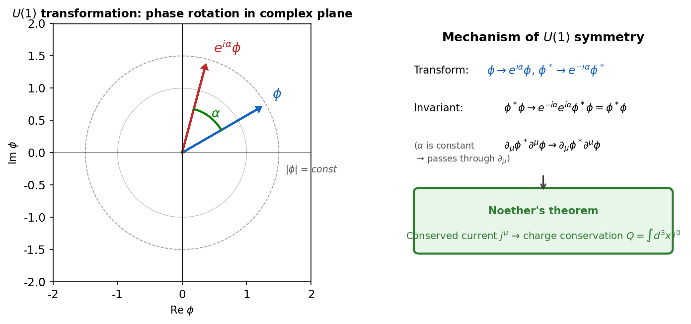
Fig. 3.5: Geometric image of the \(U(1)\) phase transformation. When \(e^{i\alpha}\) is multiplied to the field \(\phi\) in the complex plane, only the phase rotates by angle \(\alpha\) while the magnitude \(|\phi|\) is preserved. Since the Lagrangian depends only on \(|\phi|^2 = \phi^*\phi\), it is invariant under this transformation, and Noether's theorem yields charge conservation.
Here \(\alpha\) is a constant real parameter.
🔵 Kai: This is a transformation that rotates only the phase without changing the magnitude of \(\phi\). Since \(|\phi|^2 = \phi^*\phi\) doesn't change, the \(m^2\phi^*\phi\) term is invariant. For \(\partial_\mu\phi^*\,\partial^\mu\phi\)... ah, but I'm worried whether \(\partial_\mu\) acts on \(e^{i\alpha}\) for the term with derivatives.
🟡 Lina: Good observation. But since \(\alpha\) is a constant (independent of \(x\)), \(\partial_\mu(e^{i\alpha}\phi) = e^{i\alpha}\partial_\mu\phi\)—\(e^{i\alpha}\) can be pulled outside the derivative. Therefore \(\partial_\mu\phi^*\,\partial^\mu\phi \to e^{-i\alpha}\partial_\mu\phi^* \cdot e^{i\alpha}\partial^\mu\phi = \partial_\mu\phi^*\,\partial^\mu\phi\). Indeed invariant.
This transformation is called the \(U(1)\) symmetry. \(U(1)\) refers to "the collection of complex numbers \(e^{i\alpha}\) with absolute value 1." These are closed under multiplication (\(e^{i\alpha_1} \times e^{i\alpha_2} = e^{i(\alpha_1 + \alpha_2)}\) is again a complex number with absolute value 1), have an inverse (multiplying by \(e^{-i\alpha}\) returns to 1), and have an identity element (the "do nothing" transformation \(e^{i \cdot 0} = 1\)). In mathematics, such a "collection that is closed under an operation (combining two elements doesn't leave the collection), has a 'do nothing' operation (identity), and has a reversing operation (inverse) for every element" is called a group. The Lorentz group from Ch. 2 has the same meaning—performing two Lorentz transformations in succession gives another Lorentz transformation (closed), there's a "do nothing" transformation (identity), and every transformation has an inverse (inverse element). The \(U\) in \(U(1)\) stands for unitary, and the \((1)\) means \(1 \times 1\) matrices—just complex numbers.
Derivation of the Conserved Current
🟡 Lina: Let's apply Noether's theorem. For an infinitesimal transformation (small \(\alpha\)), \(e^{i\alpha} \approx 1 + i\alpha\), so:
For complex fields, we treat \(\phi\) and \(\phi^*\) as independent fields. You might think "\(\phi^*\) is determined by \(\phi\), so how can they be independent?" but when we write \(\phi = \frac{1}{\sqrt{2}}(\phi_1 + i\phi_2)\), the real part \(\phi_1\) and imaginary part \(\phi_2\) are indeed two independent real fields, right? Since \(\phi\) and \(\phi^*\) are linear combinations of \(\phi_1\) and \(\phi_2\), "taking variations with respect to \(\phi\) and \(\phi^*\)" gives the same information as "taking variations with respect to \(\phi_1\) and \(\phi_2\)"—just a different choice of variables, with the same number of independent degrees of freedom: two. The conserved current is a generalization of equation (3.22). Equation (3.22) was for the case of a single field (\(\phi\) only), but now we have two independent fields, \(\phi\) and \(\phi^*\). Let's consider the case of multiple fields. Writing the multi-variable version of equation (3.17): \(\delta\mathcal{L} = \sum_a\left[\frac{\partial\mathcal{L}}{\partial\phi_a}\delta\phi_a + \frac{\partial\mathcal{L}}{\partial(\partial_\mu\phi_a)}\delta(\partial_\mu\phi_a)\right]\)—just adding up contributions from each field. This is like the total differential of a multivariable function, where for multiple variables \(\phi_1, \phi_2, \ldots\), you add up each variable's partial derivative times its change. For example, the total differential of a two-variable function \(f(u, v)\) can be written as \(df = \frac{\partial f}{\partial u}du + \frac{\partial f}{\partial v}dv\)—exactly the same structure, with \(u\) and \(v\) corresponding to \(\phi\) and \(\phi^*\).
Repeating exactly the same procedure as equations (3.18)–(3.21) for this multi-variable version: we perform integration by parts for each field \(\phi_a\), and eliminate using the Euler-Lagrange equation (which holds independently for each field). The key point is that the Euler-Lagrange equation for \(\phi\) comes from the variation of \(\phi\), and the equation for \(\phi^*\) comes from the variation of \(\phi^*\)—each vanishes independently, so what remains is only the sum of total derivative terms from each field. As a result, the conserved current is the sum of contributions from each field: \(j^\mu = \sum_a \frac{\partial \mathcal{L}}{\partial(\partial_\mu \phi_a)} D\phi_a\). In our case, \(\phi_a = \phi, \phi^*\) gives two terms:
Here \(D\phi = \delta\phi/\alpha = i\phi\) and \(D\phi^* = \delta\phi^*/\alpha = -i\phi^*\) (the remainder after dividing the common parameter \(\alpha\) from \(\delta\phi\) and \(\delta\phi^*\) in equation (3.40), respectively).
🟡 Lina: Now let's substitute the specific partial derivatives into equation (3.40a). For \(\mathcal{L} = \partial_\mu\phi^*\,\partial^\mu\phi - m^2\phi^*\phi\), recall that we treat \(\phi\) and \(\phi^*\) independently.
First, let's find \(\frac{\partial\mathcal{L}}{\partial(\partial_\mu\phi)}\). The important point is that when differentiating with respect to \(\phi\), we treat \(\phi^*\) as a "fixed separate variable"—just like when partially differentiating \(f(x, y) = xy\) with respect to \(x\), we treat \(y\) as a constant and get \(\partial f/\partial x = y\).
🔵 Kai: But \(\phi^*\) is the complex conjugate of \(\phi\), so once \(\phi\) is determined, \(\phi^*\) is determined too, right? Is it really "independent"?
🟡 Lina: Good question. As we confirmed earlier, writing \(\phi = \frac{1}{\sqrt{2}}(\phi_1 + i\phi_2)\) means \(\phi^* = \frac{1}{\sqrt{2}}(\phi_1 - i\phi_2)\), and we're essentially taking variations with respect to two independent real variables \(\phi_1\) and \(\phi_2\). "Differentiating independently with respect to \(\phi\) and \(\phi^*\)" is just rewriting "differentiating independently with respect to \(\phi_1\) and \(\phi_2\)" in different variables—a mathematically completely equivalent operation. So you can safely treat \(\phi^*\) as a constant when differentiating with respect to \(\phi\).
Making the metric tensor explicit: \(\partial_\alpha\phi^*\,\partial^\alpha\phi = \eta^{\alpha\beta}\partial_\alpha\phi^*\,\partial_\beta\phi\). When differentiating with respect to \(\partial_\mu\phi\), \(\partial_\alpha\phi^*\) is treated as a constant ("different variable"). Using the same approach as for the real scalar field (equation (3.10b)), differentiating \(\partial_\beta\phi\) with respect to \(\partial_\mu\phi\) gives the Kronecker delta \(\delta^\mu_\beta\):
For the real scalar field (equation (3.10b)), there was a \(\frac{1}{2}\) in \(\frac{1}{2}\eta^{\alpha\beta}\partial_\alpha\phi\,\partial_\beta\phi\), and since \(\phi\) appeared twice as the same variable, we got \(\frac{1}{2} \times 2 = 1\). This time, \(\phi^*\) and \(\phi\) are different variables, so differentiating with respect to \(\partial_\mu\phi\) only triggers the \(\partial_\beta\phi\) part once—but since there's no \(\frac{1}{2}\) to begin with, the result is still \(\partial^\mu\phi^*\) with coefficient 1.
Similarly, differentiating with respect to \(\partial_\mu\phi^*\) leaves \(\partial^\mu\phi\):
🔵 Kai: For the real scalar field (equation (3.10b)), \(\frac{\partial\mathcal{L}}{\partial(\partial_\mu\phi)} = \partial^\mu\phi\), but now \(\partial^\mu\phi^*\) appears. It's interesting that the "partner" field remains.
🟡 Lina: Good observation. For complex fields, \(\phi\) and \(\phi^*\) form a "pair," so differentiating with respect to one leaves the other. Now let's substitute into equation (3.40a). Recall \(D\phi = i\phi\) and \(D\phi^* = -i\phi^*\):
(In the second equality, I just rearranged the order of scalar products—\(\partial^\mu\phi^* \cdot i\phi = i\phi \cdot \partial^\mu\phi^*\).)
The last equality just factors out \(i\) as a common factor.
Note that by convention, some authors adopt \(j^\mu = i(\phi^*\partial^\mu\phi - \phi\,\partial^\mu\phi^*)\) (multiplied by \(-1\) overall) as the conserved current, so that particle charge comes out positive. The overall normalization of the Noether current (multiplying by a constant) is arbitrary, so both are correct. When we quantize in Ch. 4, we'll choose the normalization so that the particle charge is \(+1\), so for now just remember that "there's freedom in the choice of sign."
⚪ Mei: I was able to follow the calculation. You add contributions from the two fields and collect with \(i\) to get this form.
🔵 Kai: Is this the conserved current corresponding to charge? But \(j^0\) contains \(\dot{\phi}^*\) and \(\dot{\phi}\) with opposite signs. Does this mean both positive and negative charges appear?
🟡 Lina: Exactly! This \(j^\mu\) satisfies \(\partial_\mu j^\mu = 0\), and the corresponding conserved quantity:
corresponds to electric charge. This is precisely the field version of "\(U(1)\) symmetry → charge conservation" learned in Quantum Mechanics Ch. 26. In quantum mechanics, the phase transformation \(\psi \to e^{i\alpha}\psi\) of the wave function was linked to probability conservation, but in field theory it manifests as charge conservation.
✅ Comprehension Check: What is the physical meaning of the conserved current \(j^\mu\) derived from the \(U(1)\) symmetry of the complex scalar field?
Answer
\(j^\mu\) is a conserved current corresponding to charge density and current density in electromagnetism. The conserved quantity \(Q = \int d^3x\,j^0\) obtained by integrating \(j^0\) over all space corresponds to electric charge, and \(\partial_\mu j^\mu = 0\) (the continuity equation) represents charge conservation.
⚪ Mei: I see, the same structure as in quantum mechanics is reproduced in the language of fields. Because there's a \(U(1)\) symmetry, a conserved quantity exists, and that's the charge.
🟡 Lina: Wonderful connection. And the important point is that a real scalar field does not have \(U(1)\) symmetry. For a real field, \(\phi = \phi^*\), so phase rotation can't be performed. Therefore, particles described by a real scalar field carry no charge. A complex field is needed.
🔵 Kai: I see! Is this related to the existence of antiparticles? In Quantum Mechanics Ch. 27 we learned that "relativistic equations always produce antiparticles"...
🟡 Lina: Sharp intuition. Indeed, a complex field can describe both particles and antiparticles. States with \(Q > 0\) correspond to particles, and states with \(Q < 0\) to antiparticles. At the classical level we can only say "\(Q\) can be both positive and negative," but when we quantize in Ch. 4, particles with positive charge and antiparticles with negative charge become clearly distinguished—we'll look at this in detail there.
🔵 Kai: I'm looking forward to it. So if the universe didn't have \(U(1)\) symmetry, the concept of charge itself wouldn't exist? But conversely, who decided "why does the universe have \(U(1)\) symmetry"?
🟡 Lina: Your intuition touches the essence. In fact, the Standard Model has not only \(U(1)\) but also larger symmetry groups like \(SU(2)\) and \(SU(3)\), which define the "charges" corresponding to the weak and strong forces. Symmetries determine the classification of matter and the structure of interactions—this is a central idea in modern physics. We'll explore this in detail from Ch. 19 onward.
🔵 Kai: So symmetries determine "types of forces"... But why does nature "choose" these particular symmetries like \(U(1)\), \(SU(2)\), \(SU(3)\)? Is there an even deeper theory that explains this?
🟡 Lina: That's one of the frontier questions of modern physics. Grand unified theories and string theory aim for that answer, but it hasn't been settled yet. For now, let's focus on mastering the framework that "if you assume a symmetry, the conserved quantities and force structure are determined."
🔵 Kai: So current physics understands "what happens if there's a symmetry" but doesn't yet know "why that symmetry"—it's a state where we know only one side of the input-output relationship.
✅ Comprehension Check: Does the real scalar field Lagrangian \(\mathcal{L} = \frac{1}{2}\partial_\mu\phi\,\partial^\mu\phi - \frac{1}{2}m^2\phi^2\) have \(U(1)\) symmetry? State the reason.
Answer
No, it doesn't. Applying the \(U(1)\) transformation \(\phi \to e^{i\alpha}\phi\) would make \(\phi\) complex, contradicting the premise that it's a real scalar field. For a real field, \(\phi = \phi^*\), so there's no freedom for phase rotation. Therefore there's no \(U(1)\) symmetry and no corresponding conserved charge.
📝 Exercises:
- Derivation of the Euler-Lagrange equation and conserved current for the complex scalar field → Problem M-2. Internal Symmetry and Noether Current of the Complex Scalar Field
- Application of Noether's theorem to Lorentz transformations and derivation of the angular momentum tensor → Problem A-1. Generalization of Noether's Theorem
3.6 Catalog of Representative Field Lagrangians
🟡 Lina: By now we've acquired two powerful tools: the Euler-Lagrange equations and Noether's theorem. Finally, let me list the Lagrangians for the three fields that play the leading roles in quantum field theory. Quantization will be done in subsequent chapters, so today just confirm that "we start from these Lagrangians." The overall picture is summarized in Fig. 3.6 "Catalog of representative field Lagrangians".
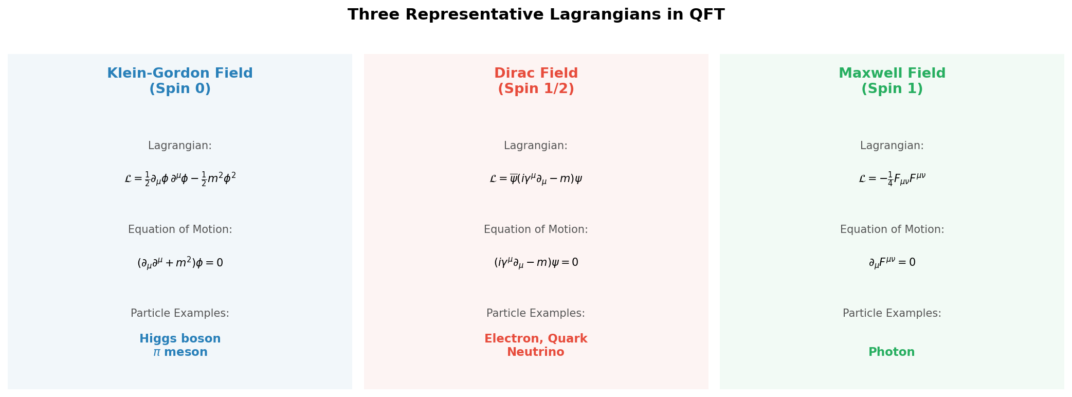
Fig. 3.6: Catalog of representative field Lagrangians. The Lagrangian catalog for the Klein-Gordon field (spin 0), Dirac field (spin 1/2), and Maxwell field (spin 1). The fundamental particles of nature are described by one of these three types.
Klein-Gordon Field (Spin 0)
🟡 Lina: First is the Klein-Gordon field that we've already been using today. It describes spin-0 particles (scalar particles).
Real scalar field:
Equation of motion: \((\partial_\mu\partial^\mu + m^2)\phi = 0\) (Klein-Gordon equation)
Complex scalar field:
🔵 Kai: The Higgs particle is a scalar particle, right?
🟡 Lina: Yes. The Higgs field is a type of complex scalar field, described by an extended version of this Lagrangian. More precisely, it has a structure that transforms under a larger symmetry (the group \(SU(2)\))—we'll treat this in detail in Ch. 19.
Dirac Field (Spin 1/2)
🟡 Lina: Next is the Dirac field. It describes spin-1/2 particles—fermions like electrons and quarks.
🔵 Kai: Wow, so many symbols... What is \(\psi\)? What's \(\bar{\psi}\)? What's \(\gamma^\mu\)?
🟡 Lina: Let me explain one by one.
- \(\psi(x)\) is a Dirac spinor: a 4-component column vector (complex-valued). While a scalar field assigns a single number to each point, a spinor field assigns 4 complex numbers to each point. As we learned in Quantum Mechanics Ch. 27, the 4 components correspond to spin up/down (2 components) × particle/antiparticle (2 sets)
- \(\bar{\psi} \equiv \psi^\dagger \gamma^0\) is the Dirac adjoint: here \(\psi^\dagger\) is the Hermitian conjugate of \(\psi\)—taking the 4-component column vector \(\psi\), laying it on its side to make a row vector (called "transpose"), and then taking the complex conjugate of each component. For example, if \(\psi = \begin{pmatrix} a \\ b \\ c \\ d \end{pmatrix}\) then \(\psi^\dagger = (a^*, b^*, c^*, d^*)\). Then multiplying \(\gamma^0\) from the right gives \(\bar{\psi}\). Why use \(\psi^\dagger\gamma^0\) rather than just \(\psi^\dagger\)? Because this makes \(\bar{\psi}\psi\) a Lorentz scalar (\(\psi^\dagger\psi\) would change value under Lorentz transformations)
- \(\gamma^\mu\) (\(\mu = 0,1,2,3\)) are the gamma matrices: \(4 \times 4\) matrices. For ordinary numbers \(ab = ba\), but matrices generally have \(AB \neq BA\). Gamma matrices satisfy an anticommutation relation. Let me define the notation: for two matrices \(A\) and \(B\), we write \(\{A, B\} \equiv AB + BA\) and call this the anticommutation relation. The commutation relation \([A, B] = AB - BA\) learned in quantum mechanics takes the "difference," but the anticommutation relation takes the "sum." Why the "sum"? We'll verify this shortly—when deriving the Klein-Gordon equation from the Dirac equation, in the calculation of \(\gamma^\mu\gamma^\nu\partial_\mu\partial_\nu\), only the symmetric part (= the anticommutation relation) survives. In other words, the anticommutation relation is naturally required as "the condition for the Dirac equation to reproduce the correct dispersion relation." The condition that gamma matrices must satisfy is: \(\{\gamma^\mu, \gamma^\nu\} = \gamma^\mu\gamma^\nu + \gamma^\nu\gamma^\mu = 2\eta^{\mu\nu}I_4\). The left side is the sum of products of \(4\times 4\) matrices, so it's a \(4\times 4\) matrix. On the right, \(\eta^{\mu\nu}\) is just a number (the \(\mu\nu\) component of the metric tensor), multiplied by the \(4\times 4\) identity matrix \(I_4\) to make it a matrix equation. For example, if \(\mu = \nu = 0\) then \(\eta^{00} = +1\) so \((\gamma^0)^2 = I_4\) (multiplying \(\gamma^0\) twice gives the identity matrix). If \(\mu = 0, \nu = 1\) then \(\eta^{01} = 0\) so \(\gamma^0\gamma^1 + \gamma^1\gamma^0 = 0\) (\(\gamma^0\) and \(\gamma^1\) "anticommute"—swapping the multiplication order flips the sign). Let me confirm why this condition is necessary.
⚪ Mei: So the anticommutation relation of gamma matrices is the consistency condition for the Dirac equation to reproduce the relativistic dispersion relation \(E^2 = |\mathbf{p}|^2 + m^2\).
First-reading guide: The following calculation is a technical verification. On first reading, it's fine to just note that "without the anticommutation relation \(\{\gamma^\mu, \gamma^\nu\} = 2\eta^{\mu\nu}\), the Dirac equation cannot reduce to the Klein-Gordon equation" and proceed to Ch. 5.
🟡 Lina: We multiply both sides of the Dirac equation \((i\gamma^\mu\partial_\mu - m)\psi = 0\) from the left by \((i\gamma^\nu\partial_\nu + m)\). Expanding gives \((i\gamma^\nu\partial_\nu + m)(i\gamma^\mu\partial_\mu - m)\psi = (i\gamma^\nu\partial_\nu)(i\gamma^\mu\partial_\mu)\psi + m(i\gamma^\mu\partial_\mu)\psi - (i\gamma^\nu\partial_\nu)(m)\psi - m^2\psi\). The second and third terms are \(im\gamma^\mu\partial_\mu\psi - im\gamma^\nu\partial_\nu\psi\), but since both \(\mu\) and \(\nu\) are dummy indices (summed over 0–3), they give the same value—they cancel to zero. What remains is \((-\gamma^\nu\gamma^\mu\partial_\nu\partial_\mu - m^2)\psi = 0\).
The key point is that \(\partial_\nu\partial_\mu\) is symmetric under exchange of \(\nu\) and \(\mu\) (\(\partial_\nu\partial_\mu = \partial_\mu\partial_\nu\)). When multiplying by something symmetric and summing, the antisymmetric part vanishes. Let me verify with a simple example. If \(a_{12} = -a_{21}\) (antisymmetric) and \(b_{12} = b_{21}\) (symmetric), then \(\sum_{i,j} a_{ij}b_{ij} = a_{12}b_{12} + a_{21}b_{21} = a_{12}b_{12} + (-a_{12})b_{12} = 0\).
🔵 Kai: I see, multiplying something symmetric with something antisymmetric and summing gives zero—so the antisymmetric part of the gamma matrices vanishes when contracted with \(\partial_\nu\partial_\mu\).
🟡 Lina: Exactly. So when computing \(\gamma^\nu\gamma^\mu\partial_\nu\partial_\mu\), the "antisymmetric part" of \(\gamma^\nu\gamma^\mu\) vanishes when multiplied by the symmetric \(\partial_\nu\partial_\mu\) and summed, and only the "symmetric part" survives. Any quantity can be decomposed into symmetric and antisymmetric parts: \(\gamma^\nu\gamma^\mu = \frac{1}{2}\underbrace{(\gamma^\nu\gamma^\mu + \gamma^\mu\gamma^\nu)}_{\text{symmetric part}} + \frac{1}{2}\underbrace{(\gamma^\nu\gamma^\mu - \gamma^\mu\gamma^\nu)}_{\text{antisymmetric part}}\). The antisymmetric part vanishes by the above argument, so only the symmetric part remains—meaning \(\gamma^\nu\gamma^\mu\partial_\nu\partial_\mu = \frac{1}{2}(\gamma^\nu\gamma^\mu + \gamma^\mu\gamma^\nu)\partial_\nu\partial_\mu = \frac{1}{2}\{\gamma^\nu, \gamma^\mu\}\partial_\nu\partial_\mu\).
Using \(\{\gamma^\nu, \gamma^\mu\} = 2\eta^{\nu\mu}\) gives \(\eta^{\nu\mu}\partial_\nu\partial_\mu = \Box\). Then \(-(\Box + m^2)\psi = 0\)—the Klein-Gordon equation is reproduced. Just as we confirmed in Quantum Mechanics Ch. 27.
In other words, the anticommutation relation of gamma matrices is the condition guaranteeing that "each component of the Dirac equation satisfies the Klein-Gordon equation." We'll confirm this again carefully when we treat the Dirac field in earnest in Ch. 5.
🔵 Kai: Does the Dirac equation \((i\gamma^\mu\partial_\mu - m)\psi = 0\) from Quantum Mechanics Ch. 27 come from this Lagrangian?
🟡 Lina: Yes, it does. Let's verify. In the same spirit as treating \(\phi\) and \(\phi^*\) independently for the complex scalar field, we treat \(\psi\) and \(\bar{\psi}\) as independent fields. Look closely at equation (3.45), \(\mathcal{L}_{\text{Dirac}} = \bar{\psi}(i\gamma^\mu\partial_\mu - m)\psi\). Notice that \(\partial_\mu\) acts only on \(\psi\), and no derivatives are attached to \(\bar{\psi}\) (\(\bar{\psi}\) is just multiplied from the left).
So let's set up the Euler-Lagrange equation (3.7) with \(\bar{\psi}\) as the "dynamical variable." Substituting \(\bar{\psi}\) for \(\phi_a\) in equation (3.7):
Look at the first term. Since \(\partial_\mu\bar{\psi}\) doesn't appear anywhere in \(\mathcal{L}\), \(\frac{\partial\mathcal{L}}{\partial(\partial_\mu\bar{\psi})} = 0\). So the first term vanishes, and the equation is simply \(\frac{\partial\mathcal{L}}{\partial\bar{\psi}} = 0\).
🔵 Kai: Since no derivative of \(\bar{\psi}\) appears in the Lagrangian, the Euler-Lagrange equation becomes very simple.
🟡 Lina: Right. Now we differentiate \(\mathcal{L} = \bar{\psi}(i\gamma^\mu\partial_\mu - m)\psi\) with respect to \(\bar{\psi}\). This has the same structure as differentiating \(f = ax\) with respect to \(a\) and getting \(x\)—since \(\bar{\psi}\) appears linearly in \(\mathcal{L}\) without any derivatives, differentiating with respect to \(\bar{\psi}\) leaves the rest \((i\gamma^\mu\partial_\mu - m)\psi\). More precisely, \(\bar{\psi}\) is a 4-component row vector, so we're differentiating with respect to each component \(\bar{\psi}_\alpha\). Writing \(\mathcal{L} = \sum_{\alpha,\beta}\bar{\psi}_\alpha\, M_{\alpha\beta}\,\psi_\beta\) (where \(M = i\gamma^\mu\partial_\mu - m\)), we get \(\frac{\partial\mathcal{L}}{\partial\bar{\psi}_\alpha} = \sum_\beta M_{\alpha\beta}\psi_\beta = [(i\gamma^\mu\partial_\mu - m)\psi]_\alpha\)—the same thing as "\(f = ax\) differentiated with respect to \(a\) gives \(x\)" happens for each component, and the result can be written in matrix form as \((i\gamma^\mu\partial_\mu - m)\psi = 0\):
This is the Dirac equation. Conversely, taking variations with respect to \(\psi\) gives an equation for \(\bar{\psi}\), but we'll treat that in detail in Ch. 5.
🔵 Kai: It's distinctive that the Lagrangian contains only first-order derivatives. The Klein-Gordon field has \((\partial_\mu\phi)^2\) which effectively gives a second-order equation of motion, but the Dirac field is first-order from the start.
🟡 Lina: Good observation. Dirac's desire to "create a first-order equation" led to the discovery of spinors and gamma matrices, as we learned in Quantum Mechanics Ch. 27.
Maxwell Field (Spin 1)
🟡 Lina: Finally, the Maxwell field—the electromagnetic field. It describes spin-1 massless particles (photons).
Here \(F_{\mu\nu}\) is the electromagnetic field tensor:
\(A^\mu = (\Phi, \mathbf{A})\) are the contravariant components of the four-potential. \(\Phi\) is the familiar scalar potential from electromagnetism, and \(\mathbf{A}\) is the vector potential. Why do we use potentials instead of the electric field \(\mathbf{E}\) and magnetic field \(\mathbf{B}\) directly? Because the Lagrangian can be more naturally constructed with potentials—\(\mathbf{E}\) and \(\mathbf{B}\) have 6 components, but \(A^\mu\) needs only 4, and from the definition \(F_{\mu\nu} = \partial_\mu A_\nu - \partial_\nu A_\mu\), half of Maxwell's equations are automatically satisfied. And combining \(\Phi\) and \(\mathbf{A}\) into 4 components is for maintaining Lorentz covariance as learned in Ch. 2—since the time component \(\Phi\) and spatial components \(\mathbf{A}\) mix under Lorentz transformations, treating them separately obscures covariance. The covariant components are \(A_\mu = \eta_{\mu\nu}A^\nu = (\Phi, -\mathbf{A})\).
🔵 Kai: Is \(F_{\mu\nu}\) something that combines the electric and magnetic fields?
🟡 Lina: Yes. The electric field \(\mathbf{E}\) and magnetic field \(\mathbf{B}\) familiar from electromagnetism are contained as components of \(F_{\mu\nu}\). Let me derive this carefully.
First, recall the definition of the electric field from electromagnetism. Using the scalar potential \(\Phi\) and vector potential \(\mathbf{A}\), each component of the electric field is \(E^i = -\partial_i\Phi - \frac{\partial A^i}{\partial t}\) (in high school physics it was just \(\mathbf{E} = -\nabla\Phi\), but when there's a time-varying vector potential, the \(-\dot{\mathbf{A}}\) term is added). Here \(A^i\) are contravariant components (the usual components of \(\mathbf{A}\) in electromagnetism), and \(\partial_i = \partial/\partial x^i\) is the ordinary spatial partial derivative. In 3-dimensional Euclidean space there's no distinction between upper and lower indices, so \(E_i = E^i\).
On the other hand, from the definition (3.48) of \(F_{\mu\nu}\) with \(\mu = 0\), \(\nu = i\):
Here \(A_0 = \Phi\), and the relation between covariant and contravariant components is \(A_i = \eta_{ij}A^j = -A^i\) (spatial components flip sign). Substituting:
So \(F_{0i} = E_i\).
🔵 Kai: Hmm, I've seen textbooks that write \(F_{0i} = -E_i\)...
🟡 Lina: That's for the opposite metric sign convention (\(\eta_{\mu\nu} = \mathrm{diag}(-1,+1,+1,+1)\)). In our convention \(\eta_{\mu\nu} = \mathrm{diag}(+1,-1,-1,-1)\), we get \(F_{0i} = E_i\). Summarizing:
- \(F_{0i} = E_i\) (time-space components correspond to the electric field)
- \(F_{ij} = \partial_i A_j - \partial_j A_i = -(\partial_i A^j - \partial_j A^i)\) (space-space components correspond to the magnetic field). Using the electromagnetism definition of the magnetic field \(\mathbf{B} = \nabla \times \mathbf{A}\) written in components: \(B_k = \epsilon_{kij}\partial_i A^j\) (\(\epsilon_{kij}\) is the Levi-Civita symbol learned in Quantum Mechanics Ch. 15). Specifically for \(k = 3\): \(B_3 = \partial_1 A^2 - \partial_2 A^1\). Meanwhile \(F_{12} = -(\partial_1 A^2 - \partial_2 A^1) = -B_3\) (since \(B_3 = \partial_1 A^2 - \partial_2 A^1\)). Similarly \(F_{13} = -(\partial_1 A^3 - \partial_3 A^1) = -(- B_2) = B_2\) (since \(B_2 = \partial_3 A^1 - \partial_1 A^3\) so \(\partial_1 A^3 - \partial_3 A^1 = -B_2\)), \(F_{23} = -(\partial_2 A^3 - \partial_3 A^2) = -B_1\) (since \(B_1 = \partial_2 A^3 - \partial_3 A^2\)). In general, \(F_{ij} = -\epsilon_{ijk}B_k\).
🔵 Kai: The electric and magnetic fields being combined into a single tensor is related to what we learned in Ch. 2 about "electric and magnetic fields mixing under Lorentz transformations."
🟡 Lina: Exactly. Index raising and lowering changes signs, which can be confusing at first, but what matters is that "\(F_{\mu\nu}\) contains both the electric and magnetic fields." Now, let's compute \(F_{\mu\nu}F^{\mu\nu}\) concretely. Since \(F_{\mu\nu}\) is antisymmetric (\(F_{\mu\nu} = -F_{\nu\mu}\)), the \(\mu = \nu\) terms are zero. The remaining independent components are the \(F_{0i}\) (electric field) and \(F_{ij}\) (magnetic field) parts. The key is the sign change when raising indices. For example, let's compute \(F^{0i} = \eta^{0\alpha}\eta^{i\beta}F_{\alpha\beta}\). Since \(\eta^{0\alpha}\) is nonzero only for \(\alpha = 0\) (\(\eta^{00} = +1\)), the sum survives only for \(\alpha = 0\): \(F^{0i} = \eta^{i\beta}F_{0\beta}\). Next, \(\eta^{i\beta}\) is nonzero only for \(\beta = i\) (\(\eta^{ii} = -1\)), so \(F^{0i} = (-1)F_{0i} = -E_i\) (raising the spatial index gives a factor of \(-1\)). Therefore \(F_{0i}F^{0i} = E_i \times (-E_i) = -\mathbf{E}^2\) (summing over \(i\)).
⚪ Mei: Each time you raise a spatial index, you get a factor of \(-1\)—this is a direct effect of the metric signature \(\mathrm{diag}(+1,-1,-1,-1)\).
🟡 Lina: In the double sum \(F_{\mu\nu}F^{\mu\nu} = \sum_{\mu}\sum_{\nu}F_{\mu\nu}F^{\mu\nu}\), \(\mu\) and \(\nu\) each independently run from 0 to 3, so the 3 terms with \((\mu, \nu) = (0, i)\) and the 3 terms with \((\mu, \nu) = (i, 0)\) appear separately (there's no double-counting—we're running \(\mu\) and \(\nu\) independently). The contribution from \((\mu, \nu) = (i, 0)\) uses the antisymmetry \(F_{i0} = -F_{0i}\) and \(F^{i0} = -F^{0i}\) to get \(F_{i0}F^{i0} = (-F_{0i})(-F^{0i}) = F_{0i}F^{0i} = -\mathbf{E}^2\), the same value as the \((0, i)\) case. Combined, the time-space contribution is \((-\mathbf{E}^2) + (-\mathbf{E}^2) = -2\mathbf{E}^2\). Now let's look at the space-space part. Raising the indices: \(F^{ij} = \eta^{i\alpha}\eta^{j\beta}F_{\alpha\beta} = (-1)(-1)F_{ij} = F_{ij}\) (raising a spatial index gives \(-1\) each time, but doing it twice they cancel). So \(F_{ij}F^{ij} = F_{ij}F_{ij}\). Counting the independent components with \(i < j\): \((i,j) = (1,2), (1,3), (2,3)\)—three in total, with \(F_{12} = -B_3\), \(F_{13} = B_2\), \(F_{23} = -B_1\). In the double sum, pairs with \(i \neq j\) appear as both \((i,j)\) and \((j,i)\), giving \(F_{ij}F^{ij} = 2(B_3^2 + B_2^2 + B_1^2) = 2\mathbf{B}^2\). In total: \(F_{\mu\nu}F^{\mu\nu} = -2\mathbf{E}^2 + 2\mathbf{B}^2 = 2(\mathbf{B}^2 - \mathbf{E}^2)\). Therefore the Lagrangian is:
Can you see the same \(L = T - V\) structure as for the Klein-Gordon field? The electric field \(\mathbf{E}\) contains time derivatives of the potential, so it's the "kinetic energy-like term," while the magnetic field \(\mathbf{B}\) involves only spatial derivatives, corresponding to the "potential-like term."
⚪ Mei: I see, the same structure as \(\frac{1}{2}\dot{\phi}^2 - \frac{1}{2}(\nabla\phi)^2\) appears for the electromagnetic field as \(\frac{1}{2}\mathbf{E}^2 - \frac{1}{2}\mathbf{B}^2\).
🟡 Lina: Exactly. And deriving the Euler-Lagrange equations from this Lagrangian yields the vacuum Maxwell equations (the other half):
This combines \(\nabla \cdot \mathbf{E} = 0\) and \(\nabla \times \mathbf{B} - \frac{\partial \mathbf{E}}{\partial t} = 0\) for vacuum (no charges or currents). For cases with charges, we need to add interaction terms to the Lagrangian—we'll treat that in Ch. 7. The other half of Maxwell's equations (\(\nabla \cdot \mathbf{B} = 0\) and \(\nabla \times \mathbf{E} + \frac{\partial \mathbf{B}}{\partial t} = 0\)) follow automatically from the definition \(F_{\mu\nu} = \partial_\mu A_\nu - \partial_\nu A_\mu\) itself.
🔵 Kai: Amazing... all of Maxwell's equations come from a single Lagrangian \(-\frac{1}{4}F_{\mu\nu}F^{\mu\nu}\).
First-reading guide: It's sufficient to remember the result \(F_{\mu\nu}F^{\mu\nu} = 2(\mathbf{B}^2 - \mathbf{E}^2)\) and that the Lagrangian becomes \(\frac{1}{2}(\mathbf{E}^2 - \mathbf{B}^2)\); the details of the index calculations above can be revisited later.
🟡 Lina: Yes. This is the power of the Lagrangian formalism. Quantization will be done in Ch. 6, where we'll face the troublesome problem of "gauge freedom."
✅ Comprehension Check: In the Maxwell field Lagrangian \(\mathcal{L} = -\frac{1}{4}F_{\mu\nu}F^{\mu\nu}\), how does the "other half" of Maxwell's equations (\(\nabla\cdot\mathbf{B}=0\) and Faraday's law) hold?
Answer
These follow automatically (as identities) from the definition of the electromagnetic field tensor \(F_{\mu\nu} = \partial_\mu A_\nu - \partial_\nu A_\mu\) itself, not from the Euler-Lagrange equations. What is derived from the Lagrangian is \(\partial_\mu F^{\mu\nu} = 0\) (\(\nabla\cdot\mathbf{E}=0\) and Ampère's law).
📝 Exercises:
- Derivation of the vacuum Maxwell equations from the Maxwell field Lagrangian → Problem A-2. Lagrangian of the Maxwell Field and Gauge Invariance
Comparison of the Three Lagrangians
🟡 Lina: Let me summarize the three fields in a table.
Table 3.5: Comparison of representative field Lagrangians
| Field | Spin | Lagrangian Density | Equation of Motion | Example Particles |
|---|---|---|---|---|
| Klein-Gordon | 0 | \(\frac{1}{2}\partial_\mu\phi\,\partial^\mu\phi - \frac{1}{2}m^2\phi^2\) | \((\Box + m^2)\phi = 0\) | Higgs particle, pions |
| Dirac | 1/2 | \(\bar{\psi}(i\gamma^\mu\partial_\mu - m)\psi\) | \((i\gamma^\mu\partial_\mu - m)\psi = 0\) | Electrons, quarks |
| Maxwell | 1 | \(-\frac{1}{4}F_{\mu\nu}F^{\mu\nu}\) | \(\partial_\mu F^{\mu\nu} = 0\) | Photons |
⚪ Mei: The fundamental particles of nature are all either spin 0, 1/2, or 1, and each has a corresponding Lagrangian. Once you write down the Lagrangian, the equations of motion, symmetries, and conserved quantities are all determined automatically.
🟡 Lina: Yes. In quantum field theory, "choosing the Lagrangian" IS "defining the theory." Even the Standard Model, when you get down to it, is just writing down a single Lagrangian. Starting from the next chapter, we'll proceed with quantization using these Lagrangians as our starting point.
🔵 Kai: So once you write the Lagrangian, the calculations proceed mechanically? But conversely, "how to find the correct Lagrangian" is the hardest problem, right?
🟡 Lina: That's exactly where physicists show their skill. "Which Lagrangian to choose" is determined by symmetry requirements and experimental data. Symmetries strongly constrain the form of the Lagrangian—this is the reverse use of Noether's theorem. You can reason: "Because this conservation law must hold, the Lagrangian must have this symmetry."
✅ Comprehension Check: In quantum field theory, what specifically does it mean to "define a theory"?
Answer
It means specifying the Lagrangian density \(\mathcal{L}(\phi_a, \partial_\mu\phi_a)\). Once the Lagrangian is determined, the equations of motion from the Euler-Lagrange equations, the conserved quantities from Noether's theorem, and (as learned in subsequent chapters) the particle scattering amplitudes from quantization procedures are all derived.
3.7 Summary of This Chapter
🟡 Lina: Let's organize what we learned today.
-
We defined the Lagrangian density \(\mathcal{L}(\phi, \partial_\mu\phi)\) and derived the field Euler-Lagrange equations by making the action \(S = \int d^4x\,\mathcal{L}\) stationary
-
We proved Noether's theorem: continuous symmetry → conserved current \(j^\mu\) (\(\partial_\mu j^\mu = 0\)) → conserved quantity \(Q = \int d^3x\,j^0\)
-
Concrete examples:
- Spacetime translation invariance → energy-momentum tensor \(T^{\mu\nu}\) → energy-momentum conservation
-
\(U(1)\) phase transformation invariance → current \(j^\mu\) → charge conservation
-
We presented the three representative Lagrangians (Klein-Gordon, Dirac, Maxwell) and confirmed their respective equations of motion
🔵 Kai: The "symmetries and conservation laws" we learned in Quantum Mechanics Ch. 26 are formulated so beautifully in the language of fields. But one thing I'm curious about—today was all about "classical" fields, right? What happens to these conserved currents and energy-momentum tensor when we quantize?
🟡 Lina: Good question. Classical conserved quantities are basically preserved in quantum theory—though a new issue of "operator ordering" arises. We'll see that in subsequent chapters.
🔵 Kai: "Operator ordering"... in quantum mechanics too, \(\hat{x}\hat{p} \neq \hat{p}\hat{x}\) and ordering matters. In quantum field theory, the field \(\phi(x)\) becomes an operator, so... in classical theory \(\phi(x)\phi(y) = \phi(y)\phi(x)\) was obvious, but once quantized, does ordering become an issue? For example, the energy density \(T^{00}\) contained \(\dot{\phi}^2\), but as an operator, how do you decide the ordering of \(\hat{\dot{\phi}}\hat{\dot{\phi}}\)...
🟡 Lina: Good question. In fact, naively writing operator products gives infinities. We handle that with a prescription called "normal ordering"—we'll see it concretely in the next chapter.
⚪ Mei: And just by writing down the Lagrangian, the equations of motion and conserved quantities are all determined. This unified framework is the starting point for quantum field theory.
🟡 Lina: Exactly. In the next chapter, we'll place the structure of quantum mechanics on top of this classical framework—that is, we'll proceed to quantize the Klein-Gordon field. Let's witness the moment when the oscillation modes of a field emerge as "particles."
Preview of Next Chapter
Ch. 4 — Quantization of the Scalar Field: Particles Born from Fields
We promote the classical field \(\phi(x)\) to an operator and impose commutation relations—carrying out the procedure of second quantization. Creation and annihilation operators emerge from the Fourier expansion of the field, and we witness the moment when "particles" naturally appear as excitations of the field.
References
- Quantum Field Theory for the Gifted Amateur (Lancaster & Blundell) Chapter 2 "Lagrangians," Chapter 6 "A first stab at canonical quantization," Chapter 8 "Examples of Lagrangians, or how to build a theory," Chapter 11 "Symmetry"
- Quantum Field Theory and the Standard Model (Schwartz) Chapter 3 "Classical field theory"
- 場の量子論 — 不変性と自由場を中心にして (Sakamoto) Chapter 9 "Review of analytical mechanics and Lagrangian formalism for fields"
- Classical Theory of Fields (Landau & Lifshitz) Chapter 2 "Relativistic Mechanics," Chapter 4 "The Electromagnetic Field Equations"
- Quantum Field Theory (David Tong, Cambridge lecture notes) Chapter 1 "Classical Field Theory"
Feedback on this page
Let us know if something was unclear, incorrect, or could be improved.