Appendix A — The Analytical Mechanics Toolbox: Functionals, Field Lagrangians, and Canonical Quantization of Fields
Story so far:
In Ch. 24, we confirmed that attempting to quantize gravity within the framework of quantum field theory hits a wall called "non-renormalizability," and we built a bridge toward string theory. From here, we enter the Appendices, which organize the mathematical tools supporting the main text to the necessary and sufficient extent.
Goals of this chapter
- Organize the toolkit of "analytical mechanics" that forms the foundation of quantum field theory, focusing specifically on elements unique to fields
- Since particle analytical mechanics (Lagrangian, Hamiltonian, Poisson brackets, canonical quantization) is assumed to have been studied in quantum mechanics Appendix D for readers following the intended reading order, we provide only a brief review here and focus on four QFT-specific points: (1) functionals and functional derivatives, (2) the field Euler-Lagrange equation, (3) canonical quantization of fields, and (4) the path integral understanding of the action principle
- Clarify the origins of the tools used repeatedly in Chapters 3–11 of the main text
A.1 Particle Analytical Mechanics (Review)
🟡 Lina: This Appendix proceeds under the assumption that you've already read Quantum Mechanics Appendix D, "Lagrangian and Hamiltonian Formalism and Canonical Quantization." If you haven't followed the reading order, or if you've forgotten the material, please look at Quantum Mechanics Quantum Mechanics Appendix D first.
🔵 Kai: What did we learn in Quantum Mechanics Quantum Mechanics Appendix D again?
🟡 Lina: The key points are condensed into this single table.
Table A.1: Correspondence between classical mechanics and quantum mechanics
| Classical Mechanics | Quantum Mechanics |
|---|---|
| Physical quantity \(A(q, p)\) (number) | Operator \(\hat{A}\) (on Hilbert space) |
| Lagrangian \(L(q, \dot{q}) = T - V\) | — |
| Action \(S[q] = \int L\,dt\) (functional) | Path integral weight \(e^{iS/\hbar}\) |
| Euler-Lagrange equation \(\frac{d}{dt}\frac{\partial L}{\partial\dot{q}} - \frac{\partial L}{\partial q} = 0\) | — |
| Canonical momentum \(p = \frac{\partial L}{\partial\dot{q}}\) | Operator \(\hat{p}\) |
| Hamiltonian \(H(q,p) = p\dot{q} - L\) | Operator \(\hat{H}\) |
| Hamilton's equations \(\dot{q} = \frac{\partial H}{\partial p}\), \(\dot{p} = -\frac{\partial H}{\partial q}\) | Heisenberg equation \(\frac{d\hat{A}}{dt} = \frac{1}{i\hbar}[\hat{A},\hat{H}]\) |
| Poisson bracket \(\{A, B\} = \frac{\partial A}{\partial q}\frac{\partial B}{\partial p} - \frac{\partial A}{\partial p}\frac{\partial B}{\partial q}\) | Commutator \(\frac{1}{i\hbar}[\hat{A}, \hat{B}]\) |
| \(\{q, p\} = 1\) | \([\hat{q}, \hat{p}] = i\hbar\) |
| Canonical quantization prescription | \(\{A, B\} \to \frac{1}{i\hbar}[\hat{A}, \hat{B}]\) |
🟡 Lina: If you trace the table from top to bottom—you construct the action \(S\) from the Lagrangian \(L = T - V\), derive the Euler-Lagrange equation from \(\delta S = 0\), move to the Hamiltonian formalism via \(H = p\dot{q} - L\), and quantize by replacing the Poisson bracket with a commutation relation.
⚪ Mei: So this table summarizes the entire picture of particle mechanics in a single page.
🟡 Lina: Exactly. In this Appendix, we focus only on the part that extends this to fields. The first tool we need is functionals and functional derivatives.
A.2 Functionals — "A Machine That Eats Functions and Returns Numbers"
🟡 Lina: First, let me introduce the concept of a "functional." This is the concept that played a central role in Chapters 10–11 (path integrals) of the main text.
🔵 Kai: How is it different from a "function"?
🟡 Lina: Let me organize the comparison.
Table A.2: Comparison of functions and functionals
| Function | Functional | |
|---|---|---|
| Input | Number | Function |
| Output | Number | Number |
| Notation | \(f(x)\) | \(F[f]\) |
A function is "a machine that returns a number when you put in a number." A functional is "a machine that returns a number when you put in an entire function."
🔵 Kai: An entire function...? I'd like a concrete example.
🟡 Lina: Let's look at a few.
Example 1: A definite integral is a functional.
If you put in \(f(x) = x^2\), you get \(F[f] = \int_0^1 x^2\,dx = \frac{1}{3}\). If you put in \(f(x) = x^3\), you get \(F[f] = \frac{1}{4}\). Different input functions give different output numbers—that's a functional.
🔵 Kai: I see, so if the "shape" of the function changes, the number changes too.
🟡 Lina: Example 2: A slightly more complex form.
Substituting \(f(x) = x^2\) gives \(G[f] = \int_0^a 5x^4\,dx = 5\cdot\frac{a^5}{5} = a^5\).
⚪ Mei: As a notational convention, parentheses \(F(x)\) mean "a number \(x\) was input," while square brackets \(F[f]\) mean "a function \(f\) was input."
🟡 Lina: Exactly. We've used this convention consistently throughout the main text.
🔵 Kai: The \(S[\phi]\) in the path integral \(\int \mathcal{D}\phi\,e^{iS[\phi]/\hbar}\) from Ch. 10 is also a functional, right? You put in the field configuration \(\phi\)—a "function"—and get back the action—a "number." ...But wait, the \(\int \mathcal{D}\phi\) in the path integral means "summing over all functions," right? What does it mean to further integrate a functional?
🟡 Lina: Good question. But that's something we covered in detail in Ch. 10 of the main text, so we won't go deep into it here. For now, it's sufficient to confirm that "\(S[\phi]\) is a functional." The action \(S[\phi]\) is the most important functional in quantum field theory.
✅ Comprehension Check: Explain the difference between a function and a functional from the perspective of "input" and "output."
Answer
A function is a correspondence where "inputting a number outputs a number." A functional is a correspondence where "inputting an entire function outputs a number." Notationally, we distinguish them by writing a function as \(f(x)\) and a functional as \(F[f]\) with square brackets.
Example 3 (slightly special): Using the Dirac delta function, you can create a functional that "picks out the value at a specific point" of a function.
🔵 Kai: We used the delta function extensively in quantum mechanics. It's "infinite" only at \(y = x\), and integrates to 1.
🟡 Lina: Right. Let me reconfirm the most important property of the delta function:
It picks out only "the value at \(x\)" of \(f\) from within the integral. This property will be used over and over from here on, so make sure you remember it well.
✅ Comprehension Check: What value does the functional \(F[f] = \int f(y)\,\delta(y - x)\,dy\), defined using the Dirac delta function, return for an input function \(f\)?
Answer
By the "picking out" property of the delta function, \(F[f] = f(x)\). That is, it is a functional that simply returns the value of the function \(f\) at the point \(x\).
✅ Comprehension Check: When you substitute \(f(x) = x\) into the functional \(M[f] = \int_0^2 [f(x)]^3\,dx\), what is the value of \(M[f]\)?
Answer
\(M[f] = \int_0^2 x^3\,dx = \left[\frac{x^4}{4}\right]_0^2 = \frac{16}{4} = 4\)
A.3 Functional Derivatives — "What Happens When You Slightly Shift a Function"
🟡 Lina: Next, let's define the "derivative" of a functional. We'll think about it by comparing with ordinary derivatives. Look at Fig. A.1 "Comparison of ordinary derivatives and functional derivatives. Left"—the left side is an ordinary derivative, showing the rate of change of the function value (the slope of the tangent) when you shift the number \(x\) by a small amount. The right side is a functional derivative, showing how the functional \(F[f]\) responds when you slightly deform the function \(f(x)\) in the neighborhood of a specific point \(x_0\).
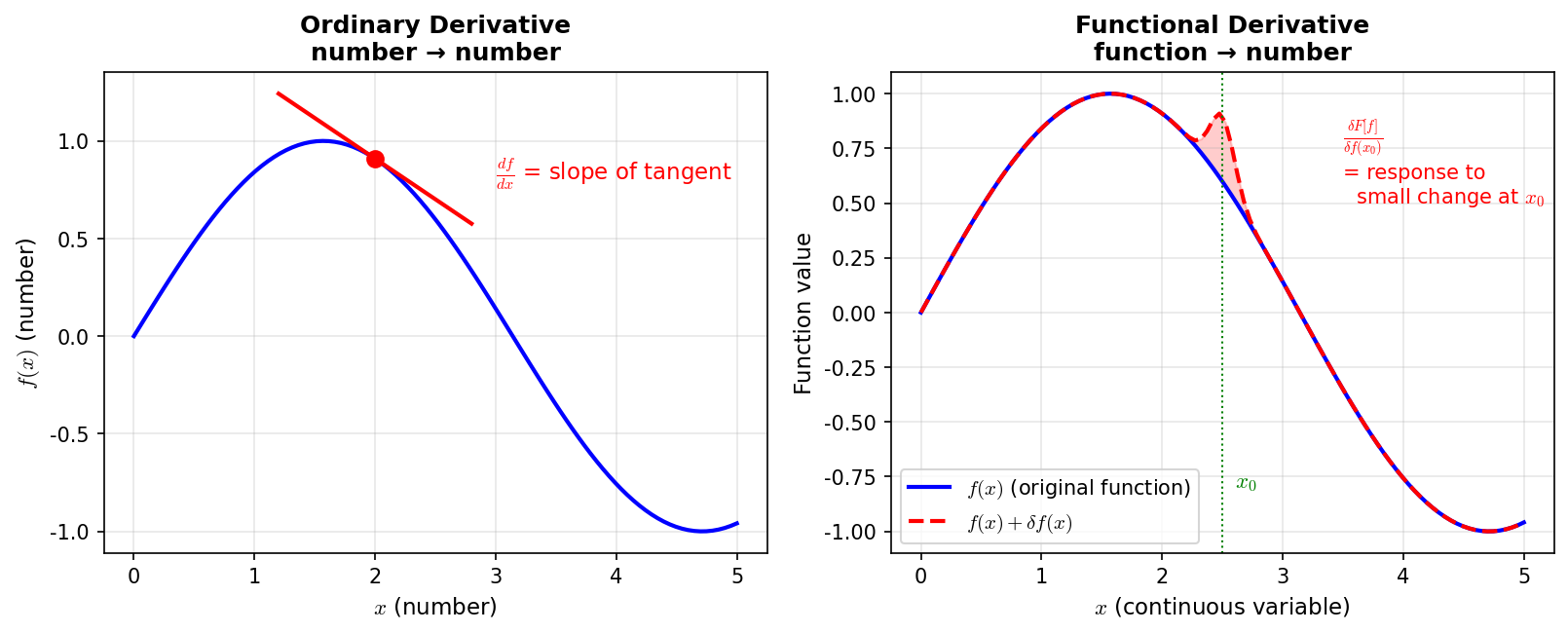
Fig. A.1: Comparison of ordinary derivatives and functional derivatives. Left — Ordinary derivative: the rate of change of the function value \(f(x)\) when the number \(x\) is shifted by a small amount (slope of tangent). Right — Functional derivative: how the functional \(F[f]\) responds when the function \(f(x)\) is slightly deformed near the point \(x_0\).
🔵 Kai: The left side of Fig. A.1 "Comparison of ordinary derivatives and functional derivatives. Left" is the familiar ordinary derivative. "How much does the output change when you slightly shift the input number"—the slope of the tangent.
The right side... shows a picture where just one point on the graph of a function is being pushed up slightly. That's the image of a functional derivative.
🟡 Lina: Exactly. The functional derivative is about examining "how much the output changes when you slightly shift the input function." Before writing the definition, let me establish a notational convention. \(x\) is a fixed point specifying "which point of the function to vary," and \(x'\) is the variable representing the argument of the function \(f\). The definition is:
For example, for an integral-type functional like \(F[f] = \int g(f(x'))\,dx'\), \(x'\) becomes the dummy variable running inside the integral. The image is: picture the graph of the function \(f\), and push it up with your finger only at the position \(x\) on the horizontal axis. The push-up amount is \(\epsilon\), and the delta function is used to push "only that point." The functional derivative shows how the functional's value responds to that push.
🔵 Kai: "Push up with your finger"—that's intuitive. But why do we shift by a delta function?
🟡 Lina: Good question. It's because we want to shift "only at point \(x\)." The delta function \(\delta(x' - x)\) has a value only at \(x' = x\), so adding \(\epsilon\,\delta(x' - x)\) to \(f(x')\) changes only the neighborhood of \(x' = x\). This way, we can determine "how the functional's value reacts when we change the function at a specific point." Let me summarize the correspondence with ordinary derivatives in a table.
Table A.3: Correspondence between ordinary derivatives and functional derivatives
| Ordinary derivative | Functional derivative | |
|---|---|---|
| Input | Number \(x\) | Function \(f(x)\) |
| Output | Number \(f(x)\) | Number \(F[f]\) |
| How to shift | \(x \to x + \epsilon\) | \(f(x') \to f(x') + \epsilon\,\delta(x'-x)\) |
| Notation | \(\frac{df}{dx}\) | \(\frac{\delta F}{\delta f(x)}\) |
⚪ Mei: Laid out like this, you can clearly see that the structures correspond perfectly.
🟡 Lina: Right. Now let's compute some concrete examples.
✅ Comprehension Check: In the definition of functional derivatives, why is the input function shifted by \(\epsilon\,\delta(x' - x)\)?
Answer
Since the delta function \(\delta(x' - x)\) has a value only at \(x' = x\), adding \(\epsilon\,\delta(x' - x)\) changes only "the neighborhood of point \(x\)" of the function. This allows us to investigate, point by point, how the functional's value responds when the function is changed at each point.
Worked Example 1
🟡 Lina: Let's find the functional derivative of \(I[f] = \int_{-1}^{1} f(y)\,dy\).
Following the definition, substitute \(f(y) \to f(y) + \epsilon\,\delta(y - x)\) (where \(y\) is the integration variable and \(x\) is the fixed point specifying "which point to change"):
The \(\int f(y)\,dy\) parts cancel between the two terms inside the brackets, leaving:
⚪ Mei: The \(\epsilon\) cancels cleanly.
🟡 Lina: The integral of the delta function is \(1\) if \(x\) is within the integration range \([-1, 1]\), and \(0\) if it's outside:
🔵 Kai: That makes intuitive sense too. \(I\) is the integral of \(f\) over \([-1,1]\), so changing \(f\) slightly within this range changes \(I\), but changing it outside the range has no effect.
Worked Example 2
🟡 Lina: Let's do a more practical example.
Here \(\varphi(y)\) is some fixed function (a weight function), and \([a, b]\) is an appropriate interval (or \((-\infty, \infty)\)).
🔵 Kai: In Worked Example 1, the integration range \([-1, 1]\) affected the result. Is it okay to omit it this time?
🟡 Lina: Good question. This time, during the calculation, the integrand takes a form with \(\delta(y-x)\) multiplied in. By the "picking out" property of the delta function \(\int g(y)\,\delta(y-x)\,dy = g(x)\), only the value at \(y = x\) is picked out and everything else vanishes. So as long as \(x\) is within the integration range, the answer is the same whether the range is \([a, b]\) or \((-\infty, \infty)\). Conversely, if \(x\) is outside the range, the result is \(0\)—the same logic as in Worked Example 1. From here on, I'll assume \(x\) is within the integration range and omit writing the limits. Let me compute the functional derivative.
Setting \(f(y) \to f(y) + \epsilon\,\delta(y - x)\):
Let's expand \([f(y) + \epsilon\,\delta(y-x)]^p\) to first order in \(\epsilon\). If we Taylor expand the function \(g(\epsilon) = (a + \epsilon b)^p\) around \(\epsilon = 0\), we get \(g(0) = a^p\), \(g'(\epsilon) = p(a+\epsilon b)^{p-1}\cdot b\), so \(g'(0) = pa^{p-1}b\). Therefore, to first order, \(g(\epsilon) \approx a^p + pa^{p-1}\cdot b\cdot\epsilon\). This is the same idea as \((1+x)^n \approx 1 + nx\) (\(|x| \ll 1\)) learned in high school—an approximation keeping only the first order in the small quantity.
🔵 Kai: Here \(b = \delta(y-x)\) is something a bit special, but we just do the same formal expansion, right?
🟡 Lina: Exactly. We're computing this purely as a "formal first-order expansion in \(\epsilon\)." The delta function by itself isn't an ordinary number, but ultimately this expansion result goes inside the integral \(\int (\cdots)\,dy\). And within the integral, it takes the form \(p[f(y)]^{p-1}\cdot\epsilon\,\delta(y-x)\cdot\varphi(y)\), so the "picking out" property of the delta function \(\int g(y)\,\delta(y-x)\,dy = g(x)\) applies directly, giving a well-defined finite value \(p[f(x)]^{p-1}\,\varphi(x)\cdot\epsilon\). In other words, even though intermediate steps may look formal, the final result is mathematically well-defined—it's justified as the operation of extracting the first-order term in \(\epsilon\). Here with \(a = f(y)\), \(b = \delta(y-x)\):
🔵 Kai: Wait a moment. Doesn't the second-order term produce something like \(\epsilon^2[\delta(y-x)]^2\)? Does the square of a delta function even make sense?
🟡 Lina: Good question. Actually, \([\delta(y-x)]^2\) doesn't have a rigorous mathematical meaning—it's a "pathological" object. But don't worry—look back at the definition of the functional derivative. Since \(\frac{\delta F}{\delta f(x)} = \lim_{\epsilon \to 0}\frac{F[f + \epsilon\delta] - F[f]}{\epsilon}\), we divide the numerator by \(\epsilon\) and then take \(\epsilon \to 0\). This means only the first-order coefficient in \(\epsilon\) survives, and second-order and higher terms (\(\epsilon^2[\delta]^2\), etc.) vanish as \(\epsilon \to 0\). So you don't need to worry about "whether \([\delta]^2\) has meaning"—that term doesn't contribute to the final result in the first place.
Substituting and canceling the \([f(y)]^p\) terms:
Finally, using the "picking out" property of the delta function:
⚪ Mei: It's exactly the same pattern as the ordinary derivative \(\frac{d}{dx}x^p = px^{p-1}\). "Lower the power by one and bring the coefficient out front."
🟡 Lina: Exactly! Since the functional derivative is the "function version of a derivative," many computational rules take the same form as ordinary differentiation.
✅ Comprehension Check: Find the functional derivative \(\frac{\delta K}{\delta f(x_0)}\) (\(0 \leq x_0 \leq 1\)) of the functional \(K[f] = \int_0^1 [f(x)]^3\,dx\).
Answer
Set \(p = 3\) and \(\varphi(y) = 1\) in Worked Example 2. \(\frac{\delta K}{\delta f(x_0)} = 3[f(x_0)]^2\).
📝 Exercises:
- Practice problems on functionals and functional derivatives → Problem B-4. Functional Derivative Using the Delta Function
A.4 The Field Euler-Lagrange Equation
🟡 Lina: The particle Euler-Lagrange equation was learned in Quantum Mechanics Quantum Mechanics Appendix D:
Here, we organize the part that extends this from "particle \(q_i(t)\)" to "field \(\phi(t, \mathbf{x})\)." This is the origin of the framework used to derive the Klein-Gordon equation in Ch. 3 of the main text.
A.4.1 Particle → Field Correspondence
🟡 Lina: Summarizing the correspondence between particle mechanics and field theory in a table:
Table A.4: Correspondence from particle mechanics to field theory
| Particle Mechanics | Field Theory |
|---|---|
| Generalized coordinates \(q_i(t)\) (finitely many) | Field \(\phi(t, \mathbf{x})\) (continuously infinite) |
| Lagrangian \(L(q, \dot{q})\) | Lagrangian density \(\mathcal{L}(\phi, \partial_\mu\phi)\) |
| Action \(S = \int dt\,L\) | Action \(S = \int d^4x\,\mathcal{L}\) |
🔵 Kai: The index \(i\) (discrete) is replaced by the coordinate \(\mathbf{x}\) (continuous). But why does the first-order time derivative \(\dot{q}\) become the 4-dimensional derivative \(\partial_\mu\phi\)? It includes spatial derivatives too, right?
🟡 Lina: Good question. There are two reasons. First, physically, since a field is spread out over space, "the difference in field values between neighboring points" contributes to the energy—imagine a chain of masses connected by springs, where the difference in displacement between neighbors generates the spring potential energy. That's why the spatial derivative \(\nabla\phi\) enters the Lagrangian.
🔵 Kai: Ah, it's the continuum limit. The stretch of springs between neighbors corresponds to the spatial derivative.
🟡 Lina: Right. And second, in special relativity, time and space are treated on equal footing, so the time derivative \(\dot{\phi}\) and spatial derivatives \(\nabla\phi\) are combined and written as the 4-dimensional derivative \(\partial_\mu\phi\). And the action \(S = \int d^4x\,\mathcal{L}\) takes the field configuration \(\phi(x)\)—a function—as input and returns the number \(S\)—a typical functional.
A.4.2 Variation and the Field Euler-Lagrange Equation
🟡 Lina: We follow the same procedure as for particles. \(\delta\phi(x)\) is the symbol representing "changing the value of the field \(\phi\) at each spacetime point by a small amount"—just like setting \(q(t) \to q(t) + \delta q(t)\) in particle mechanics. We require the condition \(\delta S = 0\) for the action \(S\) to be stationary, for arbitrary \(\delta\phi(x)\).
(Here we're summing over \(\mu\) for \(0, 1, 2, 3\)—the Einstein summation convention. This was introduced in Ch. 3 of the main text.)
First, we use \(\delta(\partial_\mu\phi) = \partial_\mu(\delta\phi)\). This means "the variation \(\delta\) and the derivative \(\partial_\mu\) can be exchanged in order."
🔵 Kai: Wait a moment. Why is it okay to swap the order?
🟡 Lina: Good question. \(\delta\phi\) is "the difference when we replace \(\phi\) with \(\phi + \delta\phi\)." Since \(\partial_\mu(\phi + \delta\phi) - \partial_\mu\phi = \partial_\mu(\delta\phi)\), we get \(\delta(\partial_\mu\phi) = \partial_\mu(\delta\phi)\). All we used here is the "linearity" of differentiation—namely the property \(\partial_\mu(A + B) = \partial_\mu A + \partial_\mu B\). Whether you take the difference first and then differentiate, or differentiate first and then take the difference, the result is the same—exactly the same logic as setting \(\delta\dot{q} = \frac{d}{dt}(\delta q)\) in particle mechanics.
🔵 Kai: I see, it comes from the linearity of differentiation. Next is integration by parts?
🟡 Lina: Right. In particle mechanics, we integrated by parts: \(\int \frac{\partial L}{\partial\dot{q}}\frac{d}{dt}(\delta q)\,dt\) became \(-\int \frac{d}{dt}\frac{\partial L}{\partial\dot{q}}\cdot\delta q\,dt\) (plus boundary terms). We do the same thing in 4 dimensions.
There are 2 key points.
- Since \(\int d^4x = \int dt\,dx\,dy\,dz\) is a multiple integral, we just perform single-variable integration by parts in each \(\mu\) direction—for example, when integrating by parts in the \(t\) direction, the \(dx\,dy\,dz\) integration just "wraps around the outside" without affecting things, so you only need to focus on the inner \(\int dt\) in \(\int dx\,dy\,dz\left[\int dt\,(\cdots)\right]\)
- The second term has a hidden sum over \(\mu\) (\(\mu = 0, 1, 2, 3\)), so we integrate by parts independently for each \(\mu\) term
In other words, there's no new technique—you just perform single-variable integration by parts, as learned in high school, once in each of the 4 directions.
⚪ Mei: Even in a multiple integral, variables other than the one you're focusing on are just "waiting on the outside," so single-variable operations suffice.
🟡 Lina: Let me concretely take out the \(\mu = 0\) (time direction) term. Since \(\int d^4x = \int dt\,dx\,dy\,dz\), we leave the integrations over non-\(t\) variables (\(dx\,dy\,dz\)) as they are and focus only on the \(t\) direction. The \(\mu = 0\) contribution from the second term is \(\frac{\partial\mathcal{L}}{\partial(\partial_0\phi)}\,\delta(\partial_0\phi)\), and using \(\delta(\partial_0\phi) = \partial_0(\delta\phi) = \frac{\partial}{\partial t}(\delta\phi)\) as confirmed earlier, the integrand becomes \(\frac{\partial\mathcal{L}}{\partial(\partial_0\phi)}\cdot\frac{\partial}{\partial t}(\delta\phi)\). This is of the form "something \(\times\) the \(t\)-derivative of \(\delta\phi\)," so single-variable integration by parts applies directly:
For \(\mu = 1\) (\(x\) direction), exactly the same approach:
Similarly for \(\mu = 2, 3\). Lining up the results of integration by parts in each of the 4 directions:
- \(\mu = 0\): \(-\frac{\partial}{\partial t}\!\left(\frac{\partial\mathcal{L}}{\partial(\partial_0\phi)}\right)\delta\phi\)
- \(\mu = 1\): \(-\frac{\partial}{\partial x}\!\left(\frac{\partial\mathcal{L}}{\partial(\partial_1\phi)}\right)\delta\phi\)
- \(\mu = 2, 3\) have the same form
Adding these 4 terms together is nothing other than the form summed over \(\mu\) using Einstein's summation convention:
🔵 Kai: Oh, even integrating by parts separately in 4 directions, everything combines into a single \(\partial_\mu\) at the end. The power of the summation convention.
🟡 Lina: Exactly. In particle mechanics, we assumed "fix the endpoints" (\(\delta q(t_1) = \delta q(t_2) = 0\)). In field theory, with the same idea, we assume "the field variation vanishes at spatial infinity" (\(\delta\phi \to 0\) as \(|x| \to \infty\)). Physically, this means "we don't change the field values at infinitely distant places or in the infinite future/past"—in other words, the natural condition that changes in the field are limited to a finite spacetime region. Under this assumption, all boundary terms vanish and:
Since \(\delta\phi\) is an arbitrary function that can be freely chosen at each spacetime point, let's think by contradiction. Suppose the contents of the brackets were nonzero at some point \(x_0\). Since the contents of the brackets form a continuous function (if \(\phi\) and \(\mathcal{L}\) are smooth), they can't suddenly become zero at nearby points—meaning the brackets maintain a nonzero value in a small region containing \(x_0\). So choose a \(\delta\phi\) that is nonzero only within that small region and zero elsewhere. Then the integral \(\int [\cdots]\delta\phi\,d^4x\) won't be zero because the brackets are nonzero in the region where \(\delta\phi\) is also nonzero—meaning \(\delta S \neq 0\). This contradicts the condition "\(\delta S = 0\) for all \(\delta\phi\)."
⚪ Mei: Proof by contradiction. "If it were nonzero at even one point, you could construct a \(\delta\phi\) that pokes just that spot, leading to a contradiction"—the same argument as for particles.
🟡 Lina: Right (this is the same argument used for particles in Quantum Mechanics Quantum Mechanics Appendix D). Therefore, the contents of the brackets must be zero at every point:
Swapping the order of terms (since \(A - B = 0\) is the same as \(B - A = 0\)), we get the form with "the derivative term first," matching the particle Euler-Lagrange equation \(\frac{d}{dt}\frac{\partial L}{\partial\dot{q}} - \frac{\partial L}{\partial q} = 0\). This is the conventional form in textbooks. This is the field Euler-Lagrange equation:
⚪ Mei: The "time derivative \(\frac{d}{dt}\)" of particle mechanics is replaced by the "4-dimensional derivative \(\partial_\mu\)" in field theory. Time and space on equal footing.
✅ Comprehension Check: What is the main difference between the particle Euler-Lagrange equation and the field Euler-Lagrange equation?
Answer
In the particle case, the total time derivative \(\frac{d}{dt}\) appears, whereas in the field case, the 4-dimensional spacetime partial derivative \(\partial_\mu\) appears. This corresponds to treating time and space on equal footing in special relativity. Additionally, the Lagrangian \(L\) is extended to the Lagrangian density \(\mathcal{L}\), and the time integral of the action \(\int dt\) is extended to the spacetime integral \(\int d^4x\).
A.4.3 Concrete Example: The Klein-Gordon Equation
🟡 Lina: Let's apply the field Euler-Lagrange equation to the Klein-Gordon field Lagrangian density treated in Ch. 3 of the main text:
Before that, let me confirm the notation. Here we're using the QFT sign convention (mostly-minus) introduced in Ch. 2 of the main text. \(\partial^\mu\phi \equiv \eta^{\mu\nu}\partial_\nu\phi\) is the derivative with the index "raised" using the Minkowski metric \(\eta^{\mu\nu} = \mathrm{diag}(+1,-1,-1,-1)\) (introduced in Ch. 3 of the main text). That is, \(\partial_\mu\phi\,\partial^\mu\phi = \eta^{\mu\nu}\partial_\mu\phi\,\partial_\nu\phi = (\partial_0\phi)^2 - (\partial_1\phi)^2 - (\partial_2\phi)^2 - (\partial_3\phi)^2\) (when the same index appears both up and down, sum over \(\mu = 0, 1, 2, 3\)—the Einstein summation convention, introduced in Ch. 3 of the main text).
🔵 Kai: Only the time component is plus, and the spatial components are minus, right?
🟡 Lina: Right. To find \(\frac{\partial\mathcal{L}}{\partial(\partial_\mu\phi)}\) needed for the Euler-Lagrange equation, let me differentiate the \(\frac{1}{2}\eta^{\alpha\beta}\partial_\alpha\phi\,\partial_\beta\phi\) part with respect to \(\partial_\mu\phi\). We treat \(\partial_0\phi, \partial_1\phi, \partial_2\phi, \partial_3\phi\) as mutually independent variables—the same idea as treating \(q\) and \(\dot{q}\) as independent variables in particle mechanics.
🔵 Kai: Wait a moment. If \(\phi\) is determined, then \(\partial_0\phi\) and \(\partial_1\phi\) are all determined too, right? Is it okay to treat them as "independent variables"?
🟡 Lina: Good question. The "treating as independent variables" here is just a convention for computing partial derivatives within the Lagrangian. In particle mechanics, when you differentiate \(L(q, \dot{q})\) with respect to \(\dot{q}\), you treat \(q\) and \(\dot{q}\) as "independent arguments of \(L\)," right? In reality, \(\dot{q} = \frac{dq}{dt}\) so once \(q(t)\) is determined, \(\dot{q}\) is also determined, but in partial derivative calculations you think of "holding one fixed and varying only the other." It's exactly the same in field theory—you treat each argument of \(\mathcal{L}(\phi, \partial_0\phi, \partial_1\phi, \partial_2\phi, \partial_3\phi)\) as independent for the purpose of calculating partial derivatives. Only after deriving the equation of motion does the relationship between \(\phi\) and \(\partial_\mu\phi\) become dynamically determined.
🔵 Kai: So it's the same as the relationship between \(q\) and \(\dot{q}\) in particle mechanics. ...But let me confirm something. In particle mechanics, only \(q\) and \(\dot{q}\)—2 things—were "independent," but in field theory, \(\phi\) and \(\partial_0\phi, \partial_1\phi, \partial_2\phi, \partial_3\phi\)—5 things—are independent? The number of variables has increased.
🟡 Lina: Good check. That's exactly right—the field Lagrangian density has 5 independent arguments: \(\mathcal{L}(\phi, \partial_0\phi, \partial_1\phi, \partial_2\phi, \partial_3\phi)\). Compared to particle mechanics where \(L(q, \dot{q})\) had 2 arguments, the number has increased by the dimensions of spacetime. Since we're treating \(\partial_0\phi, \partial_1\phi, \partial_2\phi, \partial_3\phi\) as independent variables, differentiating \(\partial_1\phi\) with respect to \(\partial_2\phi\) gives \(0\), and differentiating \(\partial_1\phi\) with respect to \(\partial_1\phi\) gives \(1\). Writing this in general: \(\frac{\partial(\partial_\alpha\phi)}{\partial(\partial_\mu\phi)} = \delta_\alpha^\mu\). \(\delta_\alpha^\mu\) is the Kronecker delta—a symbol that returns \(1\) when \(\alpha = \mu\) and \(0\) when \(\alpha \neq \mu\) (we've used it many times in the main text). Although the name is similar to the Dirac delta function \(\delta(x)\), they're completely different objects—don't confuse them. The Kronecker delta is for discrete indices, while the Dirac delta is for continuous variables.
⚪ Mei: So \(\frac{\partial(\partial_\alpha\phi)}{\partial(\partial_\mu\phi)} = \delta_\alpha^\mu\) is just writing in index notation the obvious fact that "differentiating the same variable among the 5 independent ones gives 1, and a different one gives 0."
🟡 Lina: Exactly. Using this, let's compute \(\frac{\partial}{\partial(\partial_\mu\phi)}\left(\frac{1}{2}\eta^{\alpha\beta}\partial_\alpha\phi\,\partial_\beta\phi\right)\). Since \(\eta^{\alpha\beta}\partial_\alpha\phi\,\partial_\beta\phi\) is a "product" of \(\partial_\alpha\phi\) and \(\partial_\beta\phi\), the product rule (\(\frac{\partial(AB)}{\partial C} = \frac{\partial A}{\partial C}\cdot B + A\cdot\frac{\partial B}{\partial C}\)) gives one term from the \(\alpha\) side and one from the \(\beta\) side. Specifically, differentiating the \(\alpha\) side gives \(\frac{\partial(\partial_\alpha\phi)}{\partial(\partial_\mu\phi)} = \delta_\alpha^\mu\), and differentiating the \(\beta\) side gives \(\frac{\partial(\partial_\beta\phi)}{\partial(\partial_\mu\phi)} = \delta_\beta^\mu\).
🔵 Kai: Getting 2 terms from the product rule is the same as ordinary \(\frac{d}{dx}(fg) = f'g + fg'\).
🟡 Lina: Right. Now we use the property of the Kronecker delta. In \(\eta^{\alpha\beta}\delta_\alpha^\mu\), there's a hidden sum over \(\alpha\) for \(0, 1, 2, 3\) (Einstein summation convention). Since \(\delta_\alpha^\mu\) is "1 only when \(\alpha = \mu\)," only the \(\alpha = \mu\) term survives in the sum. That is, \(\sum_\alpha \eta^{\alpha\beta}\delta_\alpha^\mu = \eta^{\mu\beta}\). Similarly, \(\eta^{\alpha\beta}\delta_\beta^\mu = \eta^{\alpha\mu}\).
🔵 Kai: Let me check. In \(\eta^{\alpha\beta}\delta_\alpha^\mu\), summing over \(\alpha\) leaves only the \(\alpha = \mu\) term, giving \(\eta^{\mu\beta}\)—so the \(\delta\) acts like it "replaces the index."
🟡 Lina: Exactly right. The most important role of the Kronecker delta is "index replacement." The result is \(\frac{1}{2}(\eta^{\mu\beta}\partial_\beta\phi + \eta^{\alpha\mu}\partial_\alpha\phi)\). Since \(\eta^{\mu\beta}\partial_\beta\phi = \partial^\mu\phi\), and \(\eta^{\alpha\mu}\partial_\alpha\phi\) is the same thing \(\partial^\mu\phi\) just with a different dummy index name, we get \(\frac{1}{2}(\partial^\mu\phi + \partial^\mu\phi) = \partial^\mu\phi\). In other words, it's the same mechanism as \(\frac{\partial(x^2)}{\partial x} = 2x\) canceling the \(\frac{1}{2}\):
⚪ Mei: The \(\frac{1}{2}\) and the 2 terms from the product rule cancel perfectly, leaving just \(\partial^\mu\phi\).
🟡 Lina: Substituting these into the field Euler-Lagrange equation \(\partial_\mu\!\left(\frac{\partial\mathcal{L}}{\partial(\partial_\mu\phi)}\right) - \frac{\partial\mathcal{L}}{\partial\phi} = 0\) gives \(\partial_\mu(\partial^\mu\phi) - (-m^2\phi) = 0\), so:
Here \(\partial_\mu(\partial^\mu\phi)\) can also be written as \(\partial_\mu\partial^\mu\phi\). In components, \(\partial_\mu\partial^\mu = \frac{\partial^2}{\partial t^2} - \frac{\partial^2}{\partial x^2} - \frac{\partial^2}{\partial y^2} - \frac{\partial^2}{\partial z^2}\), which is precisely the d'Alembert operator \(\Box \equiv \partial_\mu\partial^\mu\) introduced in Ch. 3 of the main text (QFT mostly-minus convention). Summarizing:
Or with indices made explicit: \((\partial_\mu\partial^\mu + m^2)\phi = 0\).
🔵 Kai: The Klein-Gordon equation. We derived it from the Lagrangian in Ch. 3 of the main text—and here we're confirming the grammar of that derivation.
✅ Comprehension Check: Derive the field equation of motion from the Lagrangian density \(\mathcal{L} = \frac{1}{2}\partial_\mu\phi\,\partial^\mu\phi - \frac{m^2}{2}\phi^2 - \frac{\lambda}{4!}\phi^4\).
Answer
\(\frac{\partial\mathcal{L}}{\partial\phi} = -m^2\phi - \frac{\lambda}{3!}\phi^3\), \(\frac{\partial\mathcal{L}}{\partial(\partial_\mu\phi)} = \partial^\mu\phi\). Equation of motion: \(\partial_\mu\partial^\mu\phi + m^2\phi + \frac{\lambda}{3!}\phi^3 = 0\). (Differentiating \(\phi^4\) with respect to \(\phi\) gives \(4\phi^3\), and \(\frac{1}{4!}\times 4 = \frac{1}{3!}\).)
📝 Exercises:
- Deriving Euler-Lagrange equations from various Lagrangians → Problem B-5. Application of the Euler-Lagrange Equation (1D Harmonic Oscillator)
A.5 Canonical Quantization of Fields
🟡 Lina: Canonical quantization of particles was organized as "3 steps" in Quantum Mechanics Quantum Mechanics Appendix D. The recipe replaces Poisson brackets with commutation relations. Here we extend that to fields. This is the structure behind what we wrote in Ch. 4 of the main text when we "imposed canonical commutation relations on the scalar field to quantize it."
A.5.1 Canonical Momentum Density of the Field
🟡 Lina: Corresponding to the particle canonical momentum \(p_i = \frac{\partial L}{\partial\dot{q}_i}\) is the canonical momentum density of the field:
🔵 Kai: The index \(i\) is replaced by the spatial coordinate \(\mathbf{x}\). It's like "the momentum of the \(\mathbf{x}\)-th degree of freedom."
🟡 Lina: Right. For example, for the Klein-Gordon field, let's separate the \(\mathcal{L} = \frac{1}{2}\partial_\mu\phi\,\partial^\mu\phi - \frac{m^2}{2}\phi^2\) from A.4.3 into time and spatial components. Using the metric \(\eta^{\mu\nu} = \mathrm{diag}(+1,-1,-1,-1)\), we get \(\partial_\mu\phi\,\partial^\mu\phi = (\partial_0\phi)^2 - (\partial_1\phi)^2 - (\partial_2\phi)^2 - (\partial_3\phi)^2 = \dot{\phi}^2 - (\nabla\phi)^2\), so \(\mathcal{L} = \frac{1}{2}\dot{\phi}^2 - \frac{1}{2}(\nabla\phi)^2 - \frac{m^2}{2}\phi^2\). From this, \(\pi = \frac{\partial\mathcal{L}}{\partial\dot{\phi}} = \dot{\phi}\).
A.5.2 Hamiltonian Density
🟡 Lina: Corresponding to the particle Hamiltonian \(H = p\dot{q} - L\) is the Hamiltonian density:
(If you eliminate \(\dot{\phi}\) using the relation between \(\pi\) and \(\phi\), then \(\mathcal{H}\) becomes a function of \(\phi, \pi, \nabla\phi\).)
🟡 Lina: Since it's a "density," to get the total Hamiltonian you integrate over space:
$$ H = \int d^3\mathbf{x}\;\mathcal{H} $$ ⚪ Mei: In particle mechanics, \(H\) was directly the energy, but for fields you add up the energy density at each point over all of space.
🟡 Lina: For the Klein-Gordon field, substituting \(\pi = \dot{\phi}\) and \(\mathcal{L} = \frac{1}{2}\dot{\phi}^2 - \frac{1}{2}(\nabla\phi)^2 - \frac{m^2}{2}\phi^2\):
When expanding the brackets, the minus sign applies to each term, flipping their signs:
Since \(\pi = \dot{\phi}\), we can rewrite \(\frac{1}{2}\dot{\phi}^2 = \frac{1}{2}\pi^2\):
🔵 Kai: Everything is a sum of squares—the energy density is guaranteed to be \(\geq 0\). That's reassuring.
🟡 Lina: Right, everything is in squared form and non-negative—this shows that the energy density is positive definite.
A.5.3 Field Poisson Brackets and Canonical Quantization
🟡 Lina: Corresponding to the particle Poisson bracket \(\{q_i, p_j\} = \delta_{ij}\) is the field Poisson bracket. As we saw in the correspondence table in A.4.1, the discrete index \(i\) of particle mechanics is replaced by the continuous coordinate \(\mathbf{x}\) in field theory. So the \(\delta_{ij}\) that represents "whether the \(i\)-th and \(j\)-th degrees of freedom are the same" also changes to its continuous version—\(\delta^{(3)}(\mathbf{x} - \mathbf{y})\)—which represents "whether points \(\mathbf{x}\) and \(\mathbf{y}\) are the same." Let me state the conclusion first: the fundamental relations of the field Poisson bracket are:
These are results derived from the definition of the field Poisson bracket—I'll show the definition itself shortly. Notice that the same time \(t\) appears on both sides. These are equal-time Poisson brackets evaluated at the same time \(t\). Since Poisson brackets are tools of classical mechanics, \(\hbar\) doesn't appear—\(\hbar\) enters later when we replace them with commutation relations in canonical quantization. The relations between fields at different times are determined by the equations of motion.
⚪ Mei: The Kronecker delta \(\delta_{ij}\) is replaced by the Dirac delta function \(\delta^{(3)}(\mathbf{x} - \mathbf{y})\).
🔵 Kai: Huh, why can't we use the Kronecker delta? If we're just determining whether it's the same point, \(\delta_{ij}\) seems fine.
🟡 Lina: Good question. Since the discrete indices \(i, j\) become continuous coordinates \(\mathbf{x}, \mathbf{y}\), the Kronecker delta—which is "1 only when \(i = j\)"—can't handle continuous coordinates. Instead, it naturally gets replaced by the Dirac delta, which has a "sharp peak only at \(\mathbf{x} = \mathbf{y}\)." Here \(\delta^{(3)}(\mathbf{x}-\mathbf{y})\) is the 3-dimensional version of the Dirac delta function—the 1-dimensional \(\delta(x)\) extended to 3 dimensions, written as \(\delta^{(3)}(\mathbf{x}-\mathbf{y}) = \delta(x_1-y_1)\,\delta(x_2-y_2)\,\delta(x_3-y_3)\). The "picking out" property naturally extends to \(\int f(\mathbf{y})\,\delta^{(3)}(\mathbf{x}-\mathbf{y})\,d^3\mathbf{y} = f(\mathbf{x})\).
🔵 Kai: Discrete → continuous gives \(\delta_{ij} \to \delta^{(3)}(\mathbf{x}-\mathbf{y})\). ...So the dimensions change too, right? \(\delta_{ij}\) is dimensionless, but if \(\int \delta^{(3)}(\mathbf{x}-\mathbf{y})\,d^3\mathbf{y} = 1\) holds, then since \(d^3\mathbf{y}\) has dimension \([L^3]\), \(\delta^{(3)}\) must have dimension \([L^{-3}]\). Do the dimensions match on both sides of the commutation relation?
🟡 Lina: Great observation. The short answer is yes, they do match. Let's verify. First, looking at the particle case \(\{q_i, p_j\} = \delta_{ij}\): since \(\delta_{ij}\) on the right is dimensionless, the left side must also be dimensionless. Indeed, in the Poisson bracket definition \(\{A, B\} = \frac{\partial A}{\partial q}\frac{\partial B}{\partial p} - \cdots\), the dimensions of \(q\) and \(p\) enter the denominators, so \(\{q, p\}\) is \(\frac{[q]}{[q]}\cdot\frac{[p]}{[p]} = 1\) (dimensionless), which is consistent.
Let's look at the field case. The right side of \(\{\phi(\mathbf{x}), \pi(\mathbf{y})\} = \delta^{(3)}(\mathbf{x}-\mathbf{y})\) has dimension \([L^{-3}]\) (inverse length cubed), as can be seen from \(\int \delta^{(3)}(\mathbf{x}-\mathbf{y})\,d^3\mathbf{y} = 1\). The left side must have the same dimension.
🔵 Kai: In the particle case it was dimensionless, but for fields it becomes \([L^{-3}]\)? Does that mean the Poisson bracket definition itself changes?
🟡 Lina: Yes, the definition changes. In particle mechanics, \(\{A, B\} = \sum_i\left(\frac{\partial A}{\partial q_i}\frac{\partial B}{\partial p_i} - \frac{\partial A}{\partial p_i}\frac{\partial B}{\partial q_i}\right)\)—a sum over all degrees of freedom \(i\). Substituting \(A = q_k\), \(B = p_l\) gives \(\{q_k, p_l\} = \sum_i\left(\frac{\partial q_k}{\partial q_i}\frac{\partial p_l}{\partial p_i} - 0\right) = \sum_i \delta_{ki}\delta_{li} = \delta_{kl}\), which checks out. In field theory, degrees of freedom are labeled by continuous coordinates \(\mathbf{z}\), so this sum \(\sum_i\) is replaced by a spatial integral \(\int d^3\mathbf{z}\). And the partial derivative \(\frac{\partial}{\partial q_i}\) changes to a functional derivative \(\frac{\delta}{\delta\phi(\mathbf{z})}\)—in particle mechanics it was "differentiate with respect to the \(i\)-th coordinate \(q_i\)," while in field theory it becomes "differentiate with respect to the field value \(\phi(\mathbf{z})\) at point \(\mathbf{z}\)." The functional derivative we learned in A.3 is precisely that operation.
⚪ Mei: \(\sum_i\) becomes \(\int d^3\mathbf{z}\), and partial derivatives become functional derivatives—the replacement from particles to fields is thorough.
🟡 Lina: That is, for general functionals \(A[\phi,\pi]\), \(B[\phi,\pi]\), the field Poisson bracket is defined as: $$ {A, B} = \int d^3\mathbf{z}\left[\frac{\delta A}{\delta\phi(t,\mathbf{z})}\frac{\delta B}{\delta\pi(t,\mathbf{z})} - \frac{\delta A}{\delta\pi(t,\mathbf{z})}\frac{\delta B}{\delta\phi(t,\mathbf{z})}\right] $$
Substituting \(A = \phi(t,\mathbf{x})\), \(B = \pi(t,\mathbf{y})\): $$ {\phi(t, \mathbf{x}), \pi(t, \mathbf{y})} = \int d^3\mathbf{z}\left[\frac{\delta\phi(t,\mathbf{x})}{\delta\phi(t,\mathbf{z})}\frac{\delta\pi(t,\mathbf{y})}{\delta\pi(t,\mathbf{z})} - \frac{\delta\phi(t,\mathbf{x})}{\delta\pi(t,\mathbf{z})}\frac{\delta\pi(t,\mathbf{y})}{\delta\phi(t,\mathbf{z})}\right] $$
Since the replacement \(\sum_i \to \int d^3\mathbf{z}\) introduces a dimension of \([L^3]\), the result ends up with dimension \([L^{-3}]\).
🔵 Kai: I see, so because the sum becomes an integral, the dimensions shift accordingly, and the right side becomes a Dirac delta to make things consistent.
🟡 Lina: Exactly. Let's actually compute it. Let me shift perspective slightly here. \(\phi(\mathbf{x})\) is "the value of the field \(\phi\) at point \(\mathbf{x}\)"—a specific number. But to compute the functional derivative \(\frac{\delta\phi(\mathbf{x})}{\delta\phi(\mathbf{z})}\), we need to view \(\phi(\mathbf{x})\) as "receiving the entire field configuration \(\phi\) (a function) as input and returning the value at point \(\mathbf{x}\) (a number)."
🔵 Kai: Wait, isn't \(\phi(\mathbf{x})\) just "the field value at a certain point"? Calling it a functional is confusing...
🟡 Lina: I understand the feeling. Think of it with an analogy. Imagine a table listing every student's test score in a class—this corresponds to "the entire field configuration \(\phi\)." Asking "what's Taro's score?" is the operation of receiving the entire table (function) as input and returning the number in Taro's column (number)—this is a functional. \(\phi(\mathbf{x})\) is the operation of "picking out the value at point \(\mathbf{x}\) from the entire field configuration." This is exactly the definition of a functional—recall Example 3 in A.2. There we had \(F[f] = \int f(y)\,\delta(y-x)\,dy = f(x)\). "Put in function \(f\), get back the value \(f(x)\) at point \(x\)." The current \(\phi(\mathbf{x})\) has exactly the same structure—in 3-dimensional notation, \(\phi(\mathbf{x}) = \int \phi(\mathbf{z})\,\delta^{(3)}(\mathbf{z} - \mathbf{x})\,d^3\mathbf{z}\).
🔵 Kai: I see, the operation of "looking at the whole table and reading a specific column" is a functional... It really is the same structure as Example 3.
🟡 Lina: Right. So let's apply the definition of functional derivatives directly. The form \(\phi(\mathbf{x}) = \int \phi(\mathbf{z})\,\delta^{(3)}(\mathbf{z} - \mathbf{x})\,d^3\mathbf{z}\) corresponds to Worked Example 2 in A.3 with \(p = 1\) (meaning \([f(y)]^1 = f(y)\)) and weight function \(\varphi(y) = \delta^{(3)}(\mathbf{z} - \mathbf{x})\). Setting \(p = 1\) in the Worked Example 2 result \(\frac{\delta J}{\delta f(x)} = p[f(x)]^{p-1}\varphi(x)\) leaves just \(\varphi(x)\), so we get \(\frac{\delta\phi(\mathbf{x})}{\delta\phi(\mathbf{z})} = 1 \times \delta^{(3)}(\mathbf{x} - \mathbf{z}) = \delta^{(3)}(\mathbf{x} - \mathbf{z})\).
⚪ Mei: The formula we derived before can be used directly. Building up tools pays off.
🟡 Lina: Similarly, \(\frac{\delta\pi(\mathbf{y})}{\delta\pi(\mathbf{z})} = \delta^{(3)}(\mathbf{y} - \mathbf{z})\). Meanwhile, since \(\phi\) doesn't depend on \(\pi\), \(\frac{\delta\phi(\mathbf{x})}{\delta\pi(\mathbf{z})} = 0\). Similarly, since \(\pi\) doesn't depend on \(\phi\), \(\frac{\delta\pi(\mathbf{y})}{\delta\phi(\mathbf{z})} = 0\). Therefore the second term vanishes and:
Let's look at the last step carefully. The integrand contains \(\delta^{(3)}(\mathbf{x} - \mathbf{z})\). Using the "picking out" property \(\int g(\mathbf{z})\,\delta^{(3)}(\mathbf{x} - \mathbf{z})\,d^3\mathbf{z} = g(\mathbf{x})\), and viewing \(g(\mathbf{z}) = \delta^{(3)}(\mathbf{y} - \mathbf{z})\), the result of the integral is \(g(\mathbf{x}) = \delta^{(3)}(\mathbf{y} - \mathbf{x})\). And \(\delta^{(3)}(\mathbf{y} - \mathbf{x}) = \delta^{(3)}(\mathbf{x} - \mathbf{y})\) (since the delta function is even). This is how \(\delta^{(3)}(\mathbf{x} - \mathbf{y})\) naturally emerges on the right side. In summary, in the transition from discrete to continuous, \(\delta_{ij}\) (dimensionless) changes to \(\delta^{(3)}(\mathbf{x}-\mathbf{y})\) (dimension \([L^{-3}]\)), and the spatial integral in the Poisson bracket definition compensates so that dimensions are consistent.
🔵 Kai: Let me organize this. In particle mechanics, the definition of \(\{q_i, p_j\}\) has \(\sum_i\), and the result is dimensionless. In field theory, \(\sum_i\) becomes \(\int d^3\mathbf{z}\), so an extra dimension of \([L^3]\) enters. By that amount, the right side also changes from \(\delta_{ij}\) (dimensionless) to \(\delta^{(3)}(\mathbf{x}-\mathbf{y})\) (\([L^{-3}]\)) to maintain consistency. ...By the way, what are the dimensions of \(\phi\) and \(\pi\) themselves? They're different from particle \(q\) and \(p\), right?
🟡 Lina: Good question. In natural units (\(\hbar = c = 1\)), we design the action \(S = \int d^4x\,\mathcal{L}\) to be dimensionless. As we learned in Ch. 2 of the main text, in natural units all physical quantities' dimensions are expressed as powers of mass \([M]\). Let me review just the correspondences needed here: from \(c = 1\), length and time have the same dimension \([L] = [T]\); furthermore, from \(\hbar = 1\), \([L] = [M^{-1}]\) (length has the dimension of inverse mass). The last relation comes from combining \(\hbar = 1\) and \(c = 1\)—since \(\hbar c\) has the dimension of "energy \(\times\) length," setting \(\hbar c = 1\) gives \([\text{length}] = [\text{energy}]^{-1} = [M]^{-1}\). Intuitively, \(\hbar c \approx 200\,\text{MeV}\cdot\text{fm}\), so with \(\hbar = c = 1\), "1 GeV\(^{-1}\) ≈ 0.2 fm"—meaning heavier particles are smaller (have shorter wavelengths). If you've forgotten, review Ch. 2.
🔵 Kai: Why is the action dimensionless?
🟡 Lina: Remember that in quantum mechanics, the path integral weight is \(e^{iS/\hbar}\)? The argument of an exponential must be dimensionless, so \(S/\hbar\) is dimensionless—meaning \(S\) has the same dimension as \(\hbar\). In natural units, \(\hbar = 1\) (dimensionless), so \(S\) is also dimensionless.
⚪ Mei: The argument of the exponential is dimensionless—and from that, all dimensions are determined in a chain.
🟡 Lina: Let's trace the dimensions in this unit system. Since \([L] = [M^{-1}]\), \(d^4x\) is "four lengths" with dimension \([M^{-1}]^4 = [M^{-4}]\). For \(S = \int d^4x\,\mathcal{L}\) to be dimensionless, \(\mathcal{L}\) must be \([M^4]\). Looking at \(\frac{1}{2}(\partial_\mu\phi)^2\) in the Klein-Gordon field, \(\partial_\mu = \frac{\partial}{\partial x^\mu}\) is a "dividing by length" operation so its dimension is \([L^{-1}] = [M^1]\). Since \(\mathcal{L}\) is \([M^4]\) and \((\partial_\mu\phi)^2\) must also be \([M^4]\), \(\partial_\mu\phi\) is \([M^2]\). Thus \(\phi\) is \([M^{2-1}] = [M^1]\). And since \(\pi = \dot{\phi} = \partial_0\phi\), the dimension of \(\pi\) is \([\partial_0]\times[\phi] = [M^1]\times[M^1] = [M^2]\).
🔵 Kai: I see. So can we verify the dimensions of the Poisson bracket too?
🟡 Lina: Yes. Let me verify in natural units (\(\hbar = c = 1\), length dimension is \([M^{-1}]\)). In this unit system \([L^{-3}] = [M^3]\), so what we earlier called "the dimension of \(\delta^{(3)}\) is \([L^{-3}]\)" is the same as \([M^3]\). As computed earlier, \(\frac{\delta\phi(\mathbf{x})}{\delta\phi(\mathbf{z})} = \delta^{(3)}(\mathbf{x}-\mathbf{z})\), and the dimension of \(\delta^{(3)}\) is \([M^3]\) (since \(\int \delta^{(3)}\,d^3\mathbf{z} = 1\) and \(d^3\mathbf{z}\) is \([M^{-3}]\)). Similarly, \(\frac{\delta\pi(\mathbf{y})}{\delta\pi(\mathbf{z})} = \delta^{(3)}(\mathbf{y}-\mathbf{z})\) is also \([M^3]\). Since \(\int d^3\mathbf{z}\) is \([M^{-3}]\), the total is \([M^{-3}]\times[M^3]\times[M^3] = [M^3]\). The right side \(\delta^{(3)}(\mathbf{x}-\mathbf{y})\) is also \([M^3]\), confirming consistency.
🔵 Kai: I see, everything is determined from the condition that the action is dimensionless. ...So if we write in a unit system that keeps \(\hbar\) (like SI units), the dimensions of \(\phi\) and \(\pi\) change too, and \(\hbar\) appears on the right side of the commutation relation?
🟡 Lina: Exactly. In natural units \(\hbar = 1\), so the commutation relation can be written as \([\hat{\phi}(\mathbf{x}), \hat{\pi}(\mathbf{y})] = i\,\delta^{(3)}(\mathbf{x}-\mathbf{y})\), but in a unit system where \(\hbar\) is explicit, \(i\hbar\) appears on the right side. In this Appendix, I'll proceed with intermediate calculations in natural units for simplicity, and show \(i\hbar\) explicitly in the final boxed equations.
⚪ Mei: So the boxed equations reveal the "true form" of the formulas that were written with \(\hbar = 1\) in the main text.
✅ Comprehension Check: Explain why the Kronecker delta \(\delta_{ij}\) that appears in canonical quantization of particles is replaced by the Dirac delta function \(\delta^{(3)}(\mathbf{x} - \mathbf{y})\) in canonical quantization of fields.
Answer
In particle mechanics, degrees of freedom are labeled by discrete indices \(i, j\), so "whether it's the same degree of freedom" is expressed by the Kronecker delta \(\delta_{ij}\). In field theory, degrees of freedom are labeled by continuous spatial coordinates \(\mathbf{x}, \mathbf{y}\), so "whether it's the same spatial point" needs to be expressed by the Dirac delta function \(\delta^{(3)}(\mathbf{x} - \mathbf{y})\).
🟡 Lina: And applying the canonical quantization recipe—replacing Poisson brackets with commutation relations, where \(\hbar\) enters—\(\{\ ,\ \} \to \frac{1}{i\hbar}[\ ,\ ]\) gives:
This is the starting point of Ch. 4 of the main text, the equal-time commutation relation for fields. The field version of \([\hat{q}, \hat{p}] = i\hbar\) seen in Quantum Mechanics Quantum Mechanics Appendix D. In Ch. 4 of the main text we used natural units \(\hbar = 1\) and wrote \([\hat{\phi}, \hat{\pi}] = i\,\delta^{(3)}\), but here I'm making \(\hbar\) explicit.
A.5.4 Summary of Correspondences
🟡 Lina: Listing the particle-to-field correspondence:
Table A.5: Complete correspondence between particle and field canonical quantization
| Particle Mechanics | Field Theory |
|---|---|
| Generalized coordinate \(q_i(t)\) | Field \(\phi(t, \mathbf{x})\) |
| Lagrangian \(L(q, \dot{q})\) | Lagrangian density \(\mathcal{L}(\phi, \partial_\mu\phi)\) |
| Canonical momentum \(p_i = \frac{\partial L}{\partial\dot{q}_i}\) | Canonical momentum density \(\pi = \frac{\partial\mathcal{L}}{\partial\dot{\phi}}\) |
| Hamiltonian \(H = p_i\dot{q}_i - L\) | \(H = \int d^3\mathbf{x}\,\mathcal{H}\) (\(\mathcal{H} = \pi\dot{\phi} - \mathcal{L}\)) |
| \(\{q_i, p_j\} = \delta_{ij}\) | \(\{\phi(\mathbf{x}), \pi(\mathbf{y})\} = \delta^{(3)}(\mathbf{x}-\mathbf{y})\) |
| Canonical quantization: \([\hat{q}_i, \hat{p}_j] = i\hbar\,\delta_{ij}\) | \([\hat{\phi}(\mathbf{x}), \hat{\pi}(\mathbf{y})] = i\hbar\,\delta^{(3)}(\mathbf{x}-\mathbf{y})\) |
🔵 Kai: Laid out like this, the tools we learned in particle mechanics can be used directly for fields. ...But conversely, are there cases where this correspondence breaks down? Like for gauge fields?
🟡 Lina: Good observation. Actually, for gauge fields there are "constraints" that prevent naive canonical quantization from working directly. That's exactly why "gauge fixing" was needed in Ch. 7 of the main text. But that goes beyond the scope of this Appendix, so for now understand that "for simple fields like scalar fields, this correspondence holds directly."
⚪ Mei: The heart of this Appendix is this table. The structure of tools corresponds completely between particles and fields—at least for fields without constraints.
🟡 Lina: Right. Canonical quantization of particles learned in Quantum Mechanics Quantum Mechanics Appendix D, extended to continuously infinite degrees of freedom, is quantum field theory—the tools are the same, only the objects they're applied to differ.
📝 Exercises:
- Computing canonical momentum and Hamiltonian density for fields → Problem M-2. Canonical Momentum and Hamiltonian Density of a Field
A.6 Why Does Nature Follow the Action Principle?
🟡 Lina: Finally, let me touch on one deep question. "Why does a particle (or field) choose the path (configuration) where the action is stationary?"—this was posed as a question in Quantum Mechanics Quantum Mechanics Appendix D too, but now that we're in quantum field theory, we can give a somewhat deeper answer.
🔵 Kai: It's that wonder I felt when learning Fermat's principle in high school—"how does light know the fastest path?"
🟡 Lina: Within the scope of classical mechanics, we can only say "because that's the principle." But quantum mechanics and quantum field theory provide the answer.
Recall Feynman's path integral from Chapters 10–11 of the main text. The core of the path integral is that in quantum theory, a particle (or field) "simultaneously takes all possible paths (configurations)," assigns a phase factor \(e^{iS/\hbar}\) determined by the action \(S\) as a weight to each path, and sums them all up. In the classical limit (\(\hbar \to 0\)), paths where \(S\) is not stationary have the phase \(S/\hbar\) oscillating wildly and canceling each other out. Only the neighborhood of paths where \(S\) is stationary survives—so classically, the particle appears to "choose" the path with \(\delta S = 0\).
⚪ Mei: So the action principle is explained as the classical limit of the quantum path integral.
🟡 Lina: Right. Fermat's principle works the same way. If you consider the wave nature of light, only paths where the phase is aligned (= the optical path length is stationary) constructively interfere and survive. Variational principles are "the classical limit of wave interference."
🔵 Kai: So the question "why does nature follow least action" naturally emerges from the quantum structure of "superposition of all paths." But let me confirm—"paths that aren't stationary cancel out"—how precisely do they cancel? They don't go to exactly zero, right?
🟡 Lina: Good question. They don't go to strictly zero—since \(\hbar\) is finite, there remains a "quantum fuzziness" of width \(\sim\sqrt{\hbar}\) around the classical path. But for macroscopic objects, \(S/\hbar\) is astronomically large, so even a slight deviation from the stationary point causes the phase to oscillate wildly, and it can be considered to cancel practically completely.
🔵 Kai: I see. So conversely, physicists before the path integral couldn't explain "why the action principle holds"?
🟡 Lina: That's right. In the era of Euler and Lagrange, the action principle could only be accepted as an "empirically correct axiom." Only when Feynman formulated the path integral in 1948 did the physical explanation for "why nature makes the action stationary" finally arrive. And exactly the same structure holds in quantum field theory as well. All classical field equations of motion (Klein-Gordon, Maxwell, Einstein) can be understood as the classical limit of the corresponding quantum field theory. The question "why the action principle?" is naturally answered as "the classical limit of the quantum superposition of all possible field configurations."
🔵 Kai: So what we thought was an axiom was actually a consequence of a deeper theory.
🟡 Lina: In other words, in classical mechanics, the action principle was an "axiom"—a starting point accepted without proof. But from the perspective of the quantum path integral, it becomes a "derived result." The number of axioms decreases, and more can be explained from fewer assumptions—that's what it means for a theory to become deeper.
⚪ Mei: The status of the action principle changes from "assumption" to "consequence."
🔵 Kai: So we've just gone down one level of "why," right? The path integral answered the "why" of the action principle—but then, what about the "why" of the path integral itself? "Why do we superpose all paths"—will an even deeper theory answer that?
🟡 Lina: Sharp question. At present, the structure of the path integral itself is a fundamental principle of quantum theory—an "axiom." If a deeper theory is found in the future, it too might become something "derived." But for now, this is the deepest layer.
🔵 Kai: But then, the "weight" \(e^{iS/\hbar}\) of the path integral—the "\(S\)" itself is built from the Lagrangian, right? Isn't that circular?
🟡 Lina: Good point. But it's not circular. In the path integral, all values of \(S\) are used regardless of whether \(S\) is stationary—we're not assuming \(\delta S = 0\). The fact that \(\delta S = 0\) "comes out" in the classical limit is an output, not an input assumption.
🔵 Kai: I see... the only input is "the definition of \(S\)," and "\(\delta S = 0\)" is the output. It's not assumed, yet it emerges—that's indeed not circular.
⚪ Mei: Let me organize the logic so far—the path integral just "assigns \(e^{iS/\hbar}\) to all configurations and sums them," without assuming \(\delta S = 0\). But in the classical limit, only the stationary phase survives, so \(\delta S = 0\) "emerges" as a result. The distinction between input and output is the key point.
🔵 Kai: But then another question arises. What's the principle that determines the form of \(S\)?
🟡 Lina: Symmetries (Lorentz invariance, gauge invariance) strongly constrain the form of \(S\)—as we saw in Ch. 7 of the main text. But "why those symmetries" becomes an even deeper question.
🔵 Kai: So ultimately, digging one level of "why" always produces a new "why"... But at least, the path integral answered the "why" of the action principle. That alone feels like going one level deeper.
⚪ Mei: Let me organize further. Summarizing the structure we've seen in this chapter in one line—in classical mechanics, the action principle is an "axiom"; in quantum theory, it's "derived" as the classical limit of the path integral. And the path integral itself is currently an axiom. In other words, "a deeper theory turns the axioms of a shallower theory into consequences"—a hierarchical structure. The same pattern as Newtonian mechanics becoming "derived" as a limit of relativity.
🔵 Kai: Physics is like an endless staircase. But it feels good that each time you descend a step, the previous step becomes something "explained." ...If in the future a theory is found that answers "why the path integral," then the path integral itself would be "demoted" to something derived. But then wouldn't that new theory also have a "why" remaining?
🟡 Lina: Probably. But that's not a weakness of physics—it's a strength. Because there's always a next question remaining, the exploration continues.
✅ Comprehension Check: From the perspective of the path integral, explain why a classical particle appears to "choose" the path where the action \(S\) is stationary.
Answer
In quantum theory, every path is assigned a weight \(e^{iS/\hbar}\). In the classical limit (\(\hbar \to 0\)), paths where the action \(S\) is not stationary have the phase \(S/\hbar\) oscillating wildly and cancel each other out. Only the neighborhood of paths where \(S\) is stationary have aligned phases and survive, so classically it appears that only the path with \(\delta S = 0\) is realized.
Summary
🟡 Lina: Let me list the tools organized in this Appendix.
Table A.6: Tools from this Appendix and where they're used in the main text
| Tool | Definition/Formula | Where Used in Main Text |
|---|---|---|
| Functional | \(F[f]\): function → number | Chapter 3 onward (especially Chapters 10–11, path integrals) |
| Functional derivative | \(\frac{\delta F}{\delta f(x)}\) | Ch. 11 (generating functional) |
| Field Euler-Lagrange equation | \(\partial_\mu\!\left(\frac{\partial\mathcal{L}}{\partial(\partial_\mu\phi)}\right) - \frac{\partial\mathcal{L}}{\partial\phi} = 0\) | Ch. 3 (classical field theory) |
| Canonical momentum density | \(\pi = \frac{\partial\mathcal{L}}{\partial\dot{\phi}}\) | Chapters 4–6 (canonical quantization) |
| Hamiltonian density | \(\mathcal{H} = \pi\dot{\phi} - \mathcal{L}\) | Chapters 4–6 |
| Field canonical commutation relation | \([\hat{\phi}(\mathbf{x}), \hat{\pi}(\mathbf{y})] = i\hbar\,\delta^{(3)}(\mathbf{x}-\mathbf{y})\) | Chapters 4–6 |
Particle analytical mechanics (Lagrangian, Hamiltonian, Poisson brackets, canonical quantization itself) is delegated to Quantum Mechanics Quantum Mechanics Appendix D, and we focused only on extensions specific to fields. With this, the origins of all tools used from Ch. 3 onward in the main text can be traced through Quantum Mechanics Quantum Mechanics Appendix D + this Appendix A.
Next Chapter Preview
Appendix B: Representations of the Lorentz Group and Spinors — In this Appendix, we established the framework for quantizing "fields." Next, we ask "what kind of representation space does the field live in?" We mathematically classify how fields transform under Lorentz transformations—scalar, vector, and spinor—and answer, in the language of representation theory, the questions "why 4 components?" and "why are \(\gamma\) matrices needed?" that arose when we dealt with Dirac fields and Weyl spinors in the main text.
References
- Quantum Field Theory for the Gifted Amateur (Lancaster & Blundell) Chapter 2 "Lagrangian mechanics," Chapter 6 "A first stab at relativistic quantum mechanics"
- 場の量子論 — 不変性と自由場を中心にして(坂本眞人、裳華房) Chapter 9 "Review of analytical mechanics and the Lagrangian formalism for fields"
- QM Appendix D "Lagrangian and Hamiltonian Formalism and Canonical Quantization" (details of particle analytical mechanics)
Feedback on this page
Let us know if something was unclear, incorrect, or could be improved.