Chapter 7: The Wave Function and the Schrödinger Equation¶
Story so far:
In Part II (Chapters 4–6), we used a finite-dimensional two-state system as our stage to learn the rules of probability amplitudes, the seeds of Hilbert space, and time evolution and quantum oscillations. We confirmed that the Hamiltonian \(H\) (the matrix representing energy) of a two-state system governs the time evolution of state vectors, that energy eigenstates are stationary states, and that phase differences between components of different energy produce physical oscillations. However, we have not yet been able to answer the question: "Where in space is the particle?"
Goals of this chapter
- Transition from a discrete two-state system to continuous position space, introducing the wave function \(\Psi(x,t) = \langle x|\phi(t)\rangle\) as "the probability amplitude for finding the particle at position \(x\)"
- Derive the free-particle Schrödinger equation from physically motivated arguments using de Broglie waves and classical energy relations, then extend to the general form with a potential
- Derive stationary states and the time-independent Schrödinger equation, prove conservation of probability density \(|\Psi|^2\) (the continuity equation), and establish the normalization condition and physical requirements on the wave function
- With this, we obtain the fundamental equation of quantum mechanics in a "usable" form, preparing us to solve concrete problems in subsequent chapters
7.1 From Discrete States to Continuous Space¶
🟡 Lina: In Chapters 4–6, we described systems using a finite number of basis states, like spin "up" and "down" or the two configurations of an ammonia molecule. But when an electron is flying through space, to describe "where it is"—
🔵 Kai: You need infinitely many basis states, right? Each point in space becomes one basis state?
🟡 Lina: Exactly. Using the Dirac notation introduced in Ch. 5, we write the state "the particle is at position \(x\)" as \(|x\rangle\). Since \(x\) takes continuous values, the set of basis states is infinite—in fact, continuously infinite.
⚪ Mei: In Ch. 5 we used the completeness relation \(\sum_i |i\rangle\langle i| = \hat{1}\) for a finite number of basis states \(|i\rangle\).
🟡 Lina: Right. And what happens in the continuous case—the discrete
gets replaced by
for continuous positions. This is the starting point of the position representation.
🔵 Kai: What about the orthogonality of the \(|x\rangle\) states? In the discrete case it was \(\langle i|j\rangle = \delta_{ij}\), right?
🟡 Lina: In the continuous case, instead of the Kronecker delta \(\delta_{ij}\), we use the Dirac delta function \(\delta(x - x')\):
The detailed properties of the delta function are covered in Appendix C, but for now just grasp the image. Imagine a rectangle centered at \(x'\) with width \(\epsilon\) and height \(1/\epsilon\)—its area is always \(\epsilon \times (1/\epsilon) = 1\). As \(\epsilon \to 0\), the width shrinks to zero and the height grows to infinity, but the area (integral) remains 1. This is the image of the delta function \(\delta(x - x')\)—it's zero away from \(x'\) (outside the width), has a sharp peak only near \(x = x'\), and integrates to 1 over all space.
🔵 Kai: Zero width and infinite height but area 1... that's strange.
🟡 Lina: And there's another important property—for any function \(f(x)\), \(\int f(x)\,\delta(x - x')\,dx = f(x')\) holds. Intuitively, since \(\delta(x - x')\) is zero everywhere except at \(x = x'\), it "picks out" only the value \(f(x')\) from the integral—like sifting through \(f(x)\) to extract just \(f(x')\). Remembering these three properties—"zero for \(x \neq x'\)," "integrates to 1," and "picks out function values"—is sufficient.
🔵 Kai: What does it mean physically? That \(\langle x|x'\rangle = 0\) (for \(x \neq x'\))?
🟡 Lina: It means the same thing as \(\langle i|j\rangle = 0\) (\(i \neq j\)) in the discrete case. "The state of being at position \(x\)" and "the state of being at position \(x'\)" are completely distinguishable—they're mutually exclusive. If the particle is at \(x'\), the probability of finding it at \(x \neq x'\) is zero. It sounds obvious, but this is mathematically expressed by \(\delta(x - x')\).
⚪ Mei: So in going from discrete to continuous, we just replace "sum → integral" and "\(\delta_{ij}\) → \(\delta(x-x')\)," and the structure stays the same.
🟡 Lina: Exactly. Let me summarize this correspondence.
Table 7.1: Correspondence between discrete and continuous systems
| Discrete system (Chapters 5–6) | Continuous system (position representation) |
|---|---|
| Basis states $ | i\rangle$ (finite number) |
| Orthogonality $\langle i | j\rangle = \delta_{ij}$ |
| Completeness $\sum_i | i\rangle\langle i |
| Probability amplitude $C_i = \langle i | \phi\rangle$ (complex number) |
| Probability $P_i = | C_i |
| Normalization $\sum_i | C_i |
I've depicted this transition visually in Fig. 7.1 "Transition from discrete states to continuous space". On the left is the two-state system from Chapters 5–6, and on the right is the continuous-space wave function with lattice spacing taken to zero. The lattice model in the center is the bridge from discrete to continuous that Feynman conceived, which we'll treat in detail in 7.8 "Feynman's Perspective — From Lattice to Continuous Space" later in this chapter—for now, just grasp that "there's a bridge from discrete (left) to continuous (right)."
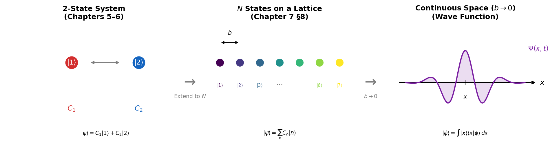
Fig. 7.1: Transition from discrete states to continuous space. Left: two-state system (Chapters 5–6). Center: \(N\) states on a lattice (Chapter 7 §8, Feynman's model). Right: as lattice spacing \(b \to 0\), the continuous-space wave function \(\Psi(x,t)\) emerges.
🟡 Lina: And when we expand an arbitrary state \(|\phi\rangle\) in the position basis states:
This is the continuous version of the discrete case \(|\phi\rangle = \sum_i |i\rangle\langle i|\phi\rangle\) (multiplying each basis state by "its component \(\langle i|\phi\rangle\)" and summing). The sum has simply become an integral. And the expansion coefficient \(\langle x|\phi\rangle\) is precisely the wave function that will be our protagonist from now on.
✅ Comprehension Check: How is the completeness relation \(\sum_i |i\rangle\langle i| = \hat{1}\) for discrete basis states replaced for continuous position basis states? And how does the orthogonality condition change?
Answer
The completeness relation becomes \(\int_{-\infty}^{+\infty} |x\rangle\langle x|\,dx = \hat{1}\), and orthogonality changes from the Kronecker delta \(\delta_{ij}\) to the Dirac delta function \(\langle x|x'\rangle = \delta(x - x')\). In the discrete-to-continuous transition, the correspondence is "sum → integral" and "\(\delta_{ij}\) → \(\delta(x-x')\)."
7.2 Superposition of de Broglie Waves and the Wave Function¶
🟡 Lina: In Ch. 2, we learned that a particle with momentum \(p\) has an associated de Broglie wavelength \(\lambda = h/p\). Here we define the wave number \(k\) as \(k = 2\pi/\lambda\). This represents "how many radians of phase the wave advances per meter." (There's an analogous quantity in the time direction—angular frequency \(\omega\)—but we'll introduce that in the next section 7.3 "The Free-Particle Schrödinger Equation — Derivation from Physical Motivation".) Now, how do we represent a wave of wavelength \(\lambda\) mathematically—it turns out we can express it as the complex exponential \(e^{ikx}\). You might think "how is \(e\) raised to an imaginary power a wave?" Using Euler's formula, it decomposes into \(\cos\) and \(\sin\), so it is indeed a wave. I'll explain this in detail shortly.
🔵 Kai: \(e^{ikx}\) is a complex number, right? How is a complex number a "wave"?
🟡 Lina: Good question. Recall Euler's formula introduced in Ch. 4:
This is the formula that says "raising \(e\) to the imaginary power \(i\theta\) gives a combination of \(\cos\) and \(\sin\)." Intuitively, it specifies a point on the unit circle in the complex plane (real axis horizontal, imaginary axis vertical) at angle \(\theta\) from the origin—when \(\theta = 0\), \(e^{i\cdot 0} = 1\) (a point on the real axis), when \(\theta = \pi/2\), \(e^{i\pi/2} = i\) (a point on the imaginary axis), and so on. The rigorous proof is deferred to Appendix B, but for now accept it as "a convenient way to package \(\cos\) and \(\sin\) into a single exponential function." Using this, \(e^{ikx} = \cos(kx) + i\sin(kx)\). So the real part is \(\cos(kx)\) and the imaginary part is \(\sin(kx)\)—both are waves of wavelength \(\lambda\). \(\cos(kx)\) completes one period every time \(kx\) increases by \(2\pi\)—meaning one period when \(x\) advances by \(2\pi/k\). From the definition \(k = 2\pi/\lambda\), we get \(2\pi/k = \lambda\), confirming it indeed represents a wave of wavelength \(\lambda\). Substituting \(\lambda = h/p\) gives \(k = 2\pi/(h/p) = 2\pi p/h = p/\hbar\) (where \(\hbar = h/(2\pi)\) is the reduced Planck constant introduced in Ch. 2). So \(e^{ikx} = e^{ipx/\hbar}\) is "the de Broglie wave corresponding to a particle of momentum \(p\), with \(\cos\) and \(\sin\) packaged into a single complex exponential." Now, following the same idea as defining \(|x\rangle\) as "the state of being at position \(x\)" in 7.1 "From Discrete States to Continuous Space", we define \(|p\rangle\) as the ket representing "the state with definite momentum value \(p\)." Then \(\langle x|p\rangle\) is "the probability amplitude for finding a particle in momentum state \(p\) at position \(x\)"—and this turns out to be a plane wave. That is, the "probability amplitude as a function of position" for a particle with definite momentum \(p\) is
a plane wave. Regarding the proportionality constant (normalization), since \(|e^{ikx}|^2 = 1\) everywhere, the integral over all space diverges, and it cannot be normalized in the usual sense—we'll discuss this again in "Normalization Condition".
🔵 Kai: But \(|e^{ikx}|^2 = 1\), uniform everywhere. You have no idea where the particle is.
🟡 Lina: Right. When momentum is definite, position becomes completely uncertain—this is a manifestation of the uncertainty principle, which we'll cover in Ch. 8. A real particle is "somewhere within a certain range of positions," so we need to superpose plane waves of different momenta to form a wave packet.
🔵 Kai: A wave packet—is that the idea of adding up waves of various wavelengths to create a "peak"?
🟡 Lina: Exactly. Just as superposing sounds of various frequencies can create a short pulse. This is the continuous version of the "superposition of probability amplitudes" we learned in Ch. 4. For a finite number of wave numbers \(k_1, k_2, \ldots, k_N\), the superposition of plane waves is \(\Psi(x) = c_1 e^{ik_1 x} + c_2 e^{ik_2 x} + \cdots = \sum_{n=1}^{N} c_n e^{ik_n x}\). Each \(c_n\) is a weight representing "how much of wave number \(k_n\) is included." Using the "sum → integral" correspondence from 7.1 "From Discrete States to Continuous Space", a superposition of continuously distributed wave numbers is written \(\Psi(x) = \int \phi(k)\,e^{ikx}\,dk\). Here \(\phi(k)\) is a weight function representing "how much of wave number \(k\) is included." The broader the range of \(k\) that \(\phi(k)\) includes, the more narrowly localized the wave packet becomes—intuitively, superposing many waves of different wavelengths makes the "peak" sharper, while using only a few wavelengths produces only a spread-out wave. This mathematical structure (Fourier transform) will be treated in detail in Ch. 8, so for now just hold the image that "adding up waves of various \(k\) can create a localized wave packet." And the state created by this superposition, expressed as "the probability amplitude at each position \(x\)," is the wave function. For a general state \(|\phi\rangle\):
This is "the probability amplitude for finding a particle in state \(|\phi(t)\rangle\) at position \(x\) at time \(t\)."
🔵 Kai: Since it's a probability amplitude, it's a complex number, right?
🟡 Lina: Yes. \(\Psi(x,t)\) is generally a complex-valued function. And applying the rule from Ch. 4—"probability is the absolute value squared of the amplitude"—to the continuous case:
We call \(|\Psi(x,t)|^2\) the probability density.
🔵 Kai: So it's not \(\Psi\) itself but \(|\Psi|^2\) that gives the probability. Since \(\Psi\) is complex, it can't directly be a probability.
🟡 Lina: To be precise, \(|\Psi|^2 = \Psi^*\Psi\). Here \(\Psi^*\) is the complex conjugate of \(\Psi\)—the imaginary part has its sign flipped. For example, if \(z = a + bi\) then \(z^* = a - bi\), and \(|z|^2 = z^*z = (a-bi)(a+bi) = a^2 + b^2\). For \(e^{i\theta}\), we have \((e^{i\theta})^* = e^{-i\theta}\), so \(|e^{i\theta}|^2 = e^{-i\theta}e^{i\theta} = e^0 = 1\).
🔵 Kai: I see, so that's why \(|e^{ikx}|^2 = 1\).
🟡 Lina: Right. Check Fig. 7.2 "Comparison of a plane wave and a wave packet. Top: A plane wave \(\Psi\propto e^{ikx}\) with definite momentum. \(|\Psi|^2\) is constant over all space, and position is completely uncertain. Bottom: A wave packet formed by superposing plane waves of different momenta. Position becomes somewhat localized, but at the cost of introducing a spread in momentum" for a visual comparison of plane waves and wave packets.
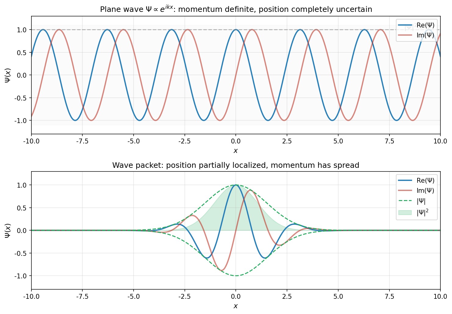
Fig. 7.2: Comparison of a plane wave and a wave packet. Top: A plane wave \(\Psi\propto e^{ikx}\) with definite momentum. \(|\Psi|^2\) is constant over all space, and position is completely uncertain. Bottom: A wave packet formed by superposing plane waves of different momenta. Position becomes somewhat localized, but at the cost of introducing a spread in momentum—this is the state of a real particle.
✅ Comprehension Check: For the wave function \(\Psi(x) \propto e^{ipx/\hbar}\) of a particle with definite momentum \(p\), what is the probability density \(|\Psi|^2\)? What does this mean physically?
Answer
\(|\Psi|^2 = |e^{ipx/\hbar}|^2 = 1\) (constant). The probability density is equal everywhere, meaning position is completely uncertain. The fact that definite momentum leads to uncertain position is a manifestation of the uncertainty principle.
7.3 The Free-Particle Schrödinger Equation — Derivation from Physical Motivation¶
🟡 Lina: Now we want to find the equation that determines how the wave function \(\Psi(x,t)\) evolves in time. In Ch. 6 we learned that the time evolution of a two-state system is described by
We're going to translate this into the position representation.
🔵 Kai: \(\hat{H}\) is the Hamiltonian—the operator representing the system's energy, right?
🟡 Lina: Right. Let's start with the simplest case—a free particle with no forces acting on it. The energy of a free particle is just kinetic energy:
Now consider the wave function of a particle with definite momentum \(p\) and energy \(E\). We'll use the de Broglie relation \(p = \hbar k\) and the Planck-Einstein relation \(E = h\nu\) from Ch. 2. Here \(\nu\) (nu) is the number of oscillations per second (frequency). Just as we absorbed \(2\pi\) into the wave number by writing \(p = \hbar k\) (\(\hbar = h/2\pi\)), it's convenient to introduce a quantity that absorbs \(2\pi\) from the frequency \(\nu\) as well. We write this as \(\omega\) (omega) and call it the angular frequency: \(\omega = 2\pi\nu\). Its meaning is "the phase (in radians) advanced per second"—the number of oscillations \(\nu\) multiplied by \(2\pi\) to convert to angle. Then \(E = h\nu = (2\pi\hbar)\cdot(\omega/2\pi) = \hbar\omega\) writes neatly. That is, just as the relationship between \(k\) and \(\hbar\) is \(p = \hbar k\), the relationship between \(\omega\) and \(\hbar\) is \(E = \hbar\omega\) with exactly the same structure. Since \(h\) and \(2\pi\) always appear together, it's more natural to use \(\hbar\) and \(\omega\) from the start. Then:
Here \(A\) is a constant (generally complex) that determines the overall magnitude of the wave function. It doesn't depend on \(x\) or \(t\), so when differentiating, we can pull \(A\) out front and differentiate only the rest. For a plane wave, \(|e^{ikx}|^2 = 1\) and the integral over all space diverges, so it cannot be normalized in the usual sense—we'll discuss this point again in "Normalization Condition". For now, don't worry about the value of \(A\) and focus on the differentiation calculations.
🔵 Kai: The spatial part \(e^{ikx}\) is the de Broglie wave, right? Where does the time part \(e^{-i\omega t}\) come from? And why is it \(e^{-i\omega t}\) with a minus sign rather than \(e^{+i\omega t}\)?
🟡 Lina: In Ch. 6, we learned that an energy eigenstate acquires a phase factor \(e^{-iEt/\hbar}\) over time. Back then, the coefficients \(C_i(t)\) of the two-state system had \(e^{-iE_n t/\hbar}\) multiplied to them, but in the position representation exactly the same thing happens—if the wave function \(\Psi(x,t)\) is an energy eigenstate, its time dependence also takes the form \(e^{-iEt/\hbar}\). The minus sign comes from the fact that the left side of the Schrödinger equation is \(i\hbar\frac{\partial}{\partial t}\)—that is, it has \(+i\) attached. Differentiating \(e^{-iEt/\hbar}\) with respect to \(t\) gives \(-iE/\hbar\), and multiplying by the \(i\hbar\) on the left side gives \(i\hbar \cdot (-iE/\hbar) = E\). If it were \(e^{+iEt/\hbar}\), we'd get \(-E\) instead of \(E\). So the minus sign is determined by the structure of the equation. Since \(E = \hbar\omega\), we have \(e^{-iEt/\hbar} = e^{-i\omega t}\). A particle with definite momentum \(p\) also has definite energy \(E = p^2/(2m)\), so the complete wave function is the spatial part \(e^{ikx}\) multiplied by the time phase factor \(e^{-i\omega t}\). Intuitively, \(e^{ikx}\) represents "where in space the oscillation occurs" and \(e^{-i\omega t}\) represents "how fast it oscillates in time"—multiplying both gives \(e^{i(kx - \omega t)}\), representing "a wave propagating through spacetime." That's the form of equation (7.8).
⚪ Mei: Spatially it oscillates as \(e^{ikx}\), temporally as \(e^{-i\omega t}\)—combined they give the form of equation (7.8).
🟡 Lina: By the way, \(e^{i(kx - \omega t)}\) represents a "wave traveling to the right." If you track a point of constant phase (\(kx - \omega t = \text{const}\)), it moves as \(x = \omega t/k + \text{const}\) with velocity \(v = \omega/k\) to the right.
🟡 Lina: Now, to connect this plane wave to the Schrödinger equation, we need to differentiate \(\Psi(x,t)\) with respect to \(t\) and \(x\). Let me review partial derivatives here. A partial derivative means "differentiating with respect to one variable while holding the others fixed" for functions of two or more variables. Since \(\Psi(x,t)\) depends on both \(x\) and \(t\), instead of the ordinary \(\frac{d}{dt}\), we use \(\frac{\partial}{\partial t}\) (the \(\partial\) symbol is called "round d" or "partial") to mean "differentiate with respect to \(t\) while holding \(x\) fixed." Similarly, \(\frac{\partial}{\partial x}\) means "differentiate with respect to \(x\) while holding \(t\) fixed." The calculation method is exactly the same as ordinary differentiation—you just "treat the other variables as constants." For example, if \(f(x,t) = x^2 t\), then \(\frac{\partial f}{\partial t} = x^2\) (treating \(x^2\) as a constant), \(\frac{\partial f}{\partial x} = 2xt\) (treating \(t\) as a constant). Simple, right?
🔵 Kai: Oh, you just treat one side as a constant. Same calculation as ordinary differentiation.
🟡 Lina: Right. Now let's proceed. In high school Math III, you learned that the derivative of \(e^x\) is \(e^x\) (\(e^x\) is the unique function that "returns to itself when differentiated"). Using the chain rule (composite function differentiation)—"differentiate the outer function, then multiply by the derivative of the inside"—differentiating \(e^{\alpha t}\) with respect to \(t\) gives \(\alpha e^{\alpha t}\). In fact, this formula holds even when \(\alpha\) is complex—recalling from Euler's formula that \(e^{i\theta} = \cos\theta + i\sin\theta\), you can verify this from the differentiation formulas for \(\cos\) and \(\sin\) (details in Appendix B). Let me quickly verify: differentiating \(e^{i\theta} = \cos\theta + i\sin\theta\) with respect to \(\theta\) gives \(-\sin\theta + i\cos\theta = i(\cos\theta + i\sin\theta) = ie^{i\theta}\)—indeed the same rule "the coefficient in the exponent comes down in front" holds just as in the real case. For now, let's accept that "complex exponential functions follow the same differentiation formulas as real ones" and proceed.
🔵 Kai: So differentiating \(e^{i\theta}\) with respect to \(\theta\) gives \(ie^{i\theta}\), just like the real case.
🟡 Lina: Exactly. Here we need the partial derivative of \(\Psi = Ae^{i(px - Et)/\hbar}\) with respect to \(t\), so we differentiate with respect to \(t\) only while holding \(x\) fixed. Holding \(x\) fixed means the \(e^{ipx/\hbar}\) part is treated as a constant. Expanding the exponent: \(\frac{i(px - Et)}{\hbar} = \frac{ipx}{\hbar} - \frac{iEt}{\hbar}\), and the coefficient of \(t\) is \(-\frac{iE}{\hbar}\). Since differentiating \(e^{\alpha t}\) with respect to \(t\) gives \(\alpha e^{\alpha t}\), with \(\alpha = -iE/\hbar\):
Next, the spatial derivative. Differentiating once with respect to \(x\) gives \(\frac{\partial\Psi}{\partial x} = \frac{ip}{\hbar}\Psi\). Differentiating once more:
🔵 Kai: Ah, from equation (7.10) we get \(p^2\Psi = -\hbar^2\frac{\partial^2\Psi}{\partial x^2}\).
⚪ Mei: Each time you differentiate, "the coefficient in the exponent comes down," so differentiating twice gives the square of the coefficient.
🟡 Lina: Exactly! Now substitute this into the energy relation (7.7). Since \(E = p^2/(2m)\):
Substituting \(E\Psi = i\hbar\frac{\partial\Psi}{\partial t}\) from equation (7.9) on the left and \(p^2\Psi = -\hbar^2\frac{\partial^2\Psi}{\partial x^2}\) from equation (7.10) on the right:
🔵 Kai: Wow! Is this the free-particle Schrödinger equation? But we derived it from a specific plane wave, right? Does it hold for other wave functions too?
🟡 Lina: Good question. Equation (7.11) is actually a linear partial differential equation. "Linear" means that \(\Psi\) and its derivatives appear to the first power (not multiplied together). There are no terms like \(\Psi^2\) or \(\Psi \cdot \frac{\partial\Psi}{\partial x}\). In this case, if \(\Psi_1\) and \(\Psi_2\) are each solutions, substituting \(c_1\Psi_1 + c_2\Psi_2\) makes each term separate out, so it's still a solution. This is the superposition principle.
🔵 Kai: Ah, so there's no problem deriving it from a specific plane wave. Any wave packet is a sum of plane waves, so if each component satisfies the equation, the whole thing does too.
⚪ Mei: In other words, no matter how many plane waves of different momenta you add together, the whole still satisfies equation (7.11).
🔵 Kai: But conversely, if the equation were nonlinear—say it had a term like \(\Psi^2\)—would superposition break down?
🟡 Lina: Exactly. In the nonlinear case, \((\Psi_1 + \Psi_2)^2 \neq \Psi_1^2 + \Psi_2^2\), so adding individual solutions doesn't give a solution. The linearity of the Schrödinger equation is directly linked to the superposition principle of quantum mechanics. So any wave packet—a superposition of plane waves of different momenta—also satisfies equation (7.11). It's an equation that governs all free-particle wave functions, not just specific plane waves.
🔵 Kai: Wait a moment. In equation (7.9), \(E\) comes from the first time derivative, and in equation (7.10), \(p^2\) comes from the second spatial derivative. Why the asymmetry between first and second order?
🟡 Lina: Sharp question. This reflects the classical energy-momentum relation \(E = p^2/(2m)\)—\(E\) is a quadratic function of \(p\). If \(E\) and \(p\) had a linear relationship (like \(E = cp\)), the spatial derivative would also be first order. In fact, for photons this is the case, and a different equation emerges. The Schrödinger equation is an equation for non-relativistic particles (moving slowly compared to the speed of light).
✅ Comprehension Check: In the derivation of the free-particle Schrödinger equation (7.11), explain in your own words how the three relations "\(E = p^2/(2m)\)," "\(E = \hbar\omega\)," and "\(p = \hbar k\)" were used.
Answer
Using \(p = \hbar k\) and \(E = \hbar\omega\), the second spatial derivative of the plane wave \(e^{i(kx-\omega t)}\) extracts \(p^2\), and the first time derivative extracts \(E\). Connecting these through the classical relation \(E = p^2/(2m)\) yields a partial differential equation containing a first time derivative and a second spatial derivative.
📝 Exercises:
- Verify by direct substitution that the plane wave \(\Psi = Ae^{i(kx - \omega t)}\) satisfies equation (7.11), and find the dispersion relation between \(\omega\) and \(k\) → Problem B-1. Substituting a Plane Wave into the Free-Particle Schrödinger Equation
7.4 Introduction of the Potential and the General Schrödinger Equation¶
🟡 Lina: Real particles experience forces. The energy of a particle subject to forces is:
Here \(V(x)\) is the potential energy. It's the same concept as gravitational potential energy \(mgh\) or spring elastic energy \(\frac{1}{2}kx^2\) from high school physics.
🔵 Kai: It's just kinetic energy plus the potential.
🟡 Lina: Right. In the free-particle derivation, we rewrote both sides of \(E\Psi = \frac{p^2}{2m}\Psi\) using differential operators. With a potential, \(E = \frac{p^2}{2m} + V(x)\), so \(E\Psi = \frac{p^2}{2m}\Psi + V(x)\Psi\). The left side is still \(i\hbar\frac{\partial\Psi}{\partial t}\), and \(\frac{p^2}{2m}\Psi\) on the right gets replaced by \(-\frac{\hbar^2}{2m}\frac{\partial^2\Psi}{\partial x^2}\). The \(V(x)\Psi\) term stays as is—\(V(x)\) is a function of \(x\), not a differential operator, so it's just multiplication. The result:
This is the one-dimensional time-dependent Schrödinger equation—the fundamental equation of quantum mechanics.
⚪ Mei: The left side is time evolution, the right side is the action of the energy operator—the same structure as the equation in Ch. 6.
🟡 Lina: Exactly. This is the position-representation version of \(i\hbar\frac{d}{dt}|\psi\rangle = \hat{H}|\psi\rangle\) from Ch. 6, written out explicitly. The Hamiltonian operator in the position representation is:
The first term is the kinetic energy operator \(\hat{T} = \hat{p}^2/(2m)\), and the second is the potential energy. Here the momentum operator is:
🔵 Kai: Why does momentum become a differential operator?
🟡 Lina: Recall equation (7.10). Acting \(-i\hbar\frac{\partial}{\partial x}\) on the plane wave \(e^{ipx/\hbar}\):
So \(-i\hbar\frac{\partial}{\partial x}\) "returns \(p\) times the original" when acting on a plane wave of momentum \(p\)—it has the form of an eigenvalue equation \(\hat{p}\,\psi_p = p\,\psi_p\). \(\psi_p = e^{ipx/\hbar}\) is the eigenfunction and \(p\) is the eigenvalue.
⚪ Mei: Same structure as the eigenvalue equations we learned in Ch. 5. Acting with the operator returns a constant multiple of the original function.
🟡 Lina: Right. And \(\hat{p}^2 = (-i\hbar\frac{\partial}{\partial x})^2 = -\hbar^2\frac{\partial^2}{\partial x^2}\), so the kinetic energy operator is \(\hat{T} = -\frac{\hbar^2}{2m}\frac{\partial^2}{\partial x^2}\).
✅ Comprehension Check: When adding a potential \(V(x)\) to the free-particle Schrödinger equation, what term is added to the right side of the equation? Why is this term simply a multiplication rather than a differential operator?
Answer
The term \(V(x)\Psi\) is added to the right side. Since \(V(x)\) is a function of position \(x\) and involves no differentiation operation on the wave function, it is simply a multiplication of \(\Psi\) by \(V(x)\). This contrasts with the kinetic energy term, which is a differential operator.
✅ Comprehension Check: What do you get when you act with the momentum operator \(\hat{p} = -i\hbar\frac{\partial}{\partial x}\) on the wave function \(\Psi(x) = Ae^{ip_0 x/\hbar}\) (\(p_0 = 3\,\text{kg}\cdot\text{m/s}\))?
Answer
\(\hat{p}\Psi = -i\hbar \cdot \frac{ip_0}{\hbar}Ae^{ip_0 x/\hbar} = p_0\,Ae^{ip_0 x/\hbar} = p_0\Psi\). The momentum eigenvalue \(p_0 = 3\,\text{kg}\cdot\text{m/s}\) is extracted. When \(\hat{p}\) acts on a momentum eigenfunction, it returns the eigenvalue (the value of the momentum) as a coefficient.
📝 Exercises:
- Write down the Hamiltonian operator for the potential \(V(x) = \frac{1}{2}m\omega^2 x^2\) (harmonic oscillator) and write the Schrödinger equation explicitly → Problem B-2. Apply the momentum operator to each of the following wave functions and find the result. If it is an eigenfunction, state the eigenvalue.
7.5 Stationary States and the Time-Independent Schrödinger Equation¶
🟡 Lina: In Ch. 6, we learned that energy eigenstates only acquire a phase factor \(e^{-iE_n t/\hbar}\) over time, making them physically unchanging "stationary states." The same thing happens in the position representation.
🔵 Kai: What form does the wave function of a stationary state take?
🟡 Lina: In Ch. 6, an eigenstate of energy \(E\) only acquired the time factor \(e^{-iEt/\hbar}\). Expecting the same in the position representation, let's try writing the wave function as a product of a "spatial part" and a "time part"—this is called separation of variables:
Here \(\psi(x)\) is a function of the spatial part only. Let's substitute this into the Schrödinger equation to verify it really works. The left side:
The right side:
Dividing both sides by \(e^{-iEt/\hbar}\):
⚪ Mei: Time has completely disappeared! Since \(\psi\) is a function of \(x\) only, we can write ordinary derivatives \(d\) instead of partial derivatives \(\partial\). It's become an ordinary differential equation in \(x\) alone.
🟡 Lina: This is the time-independent Schrödinger equation. It's the equation for finding energy eigenvalues \(E\) and eigenfunctions \(\psi(x)\). In operator language:
This is the eigenvalue equation of the Hamiltonian itself.
🔵 Kai: So solving this tells us the allowed energy values?
🟡 Lina: Yes. In general, solutions satisfying the boundary conditions (conditions for the wave function to be physically meaningful) exist only for specific energy values \(E_1, E_2, E_3, \ldots\). This is energy quantization—the answer to the mystery of atomic stability from Ch. 1.
🔵 Kai: Wow, I can finally see the origin of quantization inside the equation...!
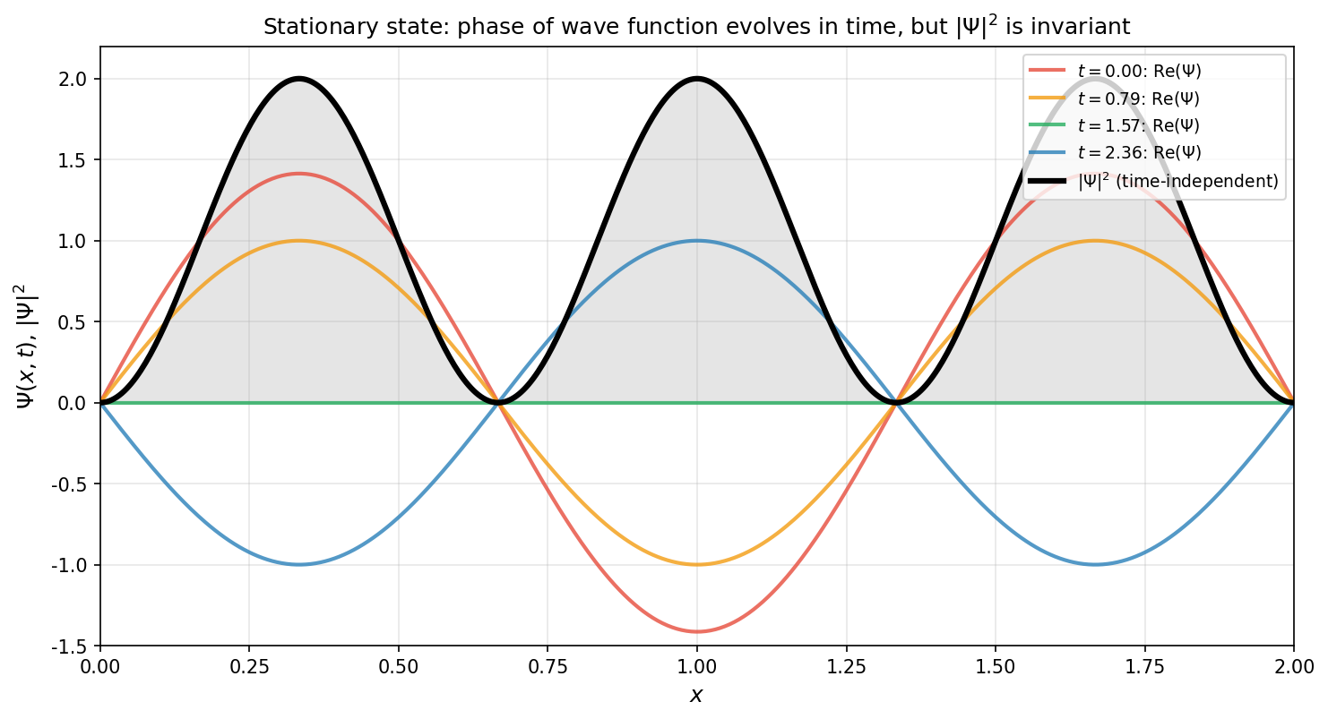
Fig. 7.3: Stationary state wave functions. An energy eigenstate \(\psi_n(x)\) acquires only a phase factor \(e^{-iE_n t/\hbar}\) over time, so the probability density \(|\Psi|^2 = |\psi_n|^2\) does not change with time — this is the meaning of "stationary."
🟡 Lina: Writing the eigenfunction corresponding to each \(E_n\) as \(\psi_n(x)\), a general wave function can be written as a superposition of these:
This is the generalization of the two-state system from Ch. 6.
⚪ Mei: The finite \(c_1, c_2\) have just become infinitely many \(c_n\)—the structure is the same.
🟡 Lina: Exactly. Each energy component has its own frequency \(\omega_n = E_n/\hbar\) at which the phase rotates. The phase difference between different energy components changes with time, causing the probability density \(|\Psi|^2\) to change over time—this is the source of dynamics in quantum systems.
🔵 Kai: Stationary states "don't change," but superposition states "move." But it's strange—each component has \(|e^{-iE_n t/\hbar}|^2 = 1\) and shouldn't affect the probability density, so why does adding them make things move?
🟡 Lina: Good question. Let's look at this concretely. We'll calculate the probability density for a superposition of two energy eigenstates \(\Psi = c_1\psi_1 e^{-iE_1 t/\hbar} + c_2\psi_2 e^{-iE_2 t/\hbar}\). Since \(|\Psi|^2 = \Psi^*\Psi\), first form \(\Psi^* = c_1^*\psi_1^* e^{iE_1 t/\hbar} + c_2^*\psi_2^* e^{iE_2 t/\hbar}\), then multiply with \(\Psi\) and expand.
🔵 Kai: Like \((A + B)(C + D)\), four terms come out.
🟡 Lina: Right. Specifically:
- \(c_1^*c_1\,\psi_1^*\psi_1 = |c_1|^2|\psi_1|^2\) (time factor \(e^{i(E_1-E_1)t/\hbar} = 1\) cancels)
- \(c_2^*c_2\,\psi_2^*\psi_2 = |c_2|^2|\psi_2|^2\) (time factor similarly cancels)
- \(c_1^*c_2\,\psi_1^*\psi_2\,e^{i(E_1-E_2)t/\hbar}\) (cross term 1)
- \(c_2^*c_1\,\psi_2^*\psi_1\,e^{i(E_2-E_1)t/\hbar}\) (cross term 2)
🔵 Kai: The first two don't depend on time, but the cross terms still have time in them—is this what causes the oscillation?
🟡 Lina: Exactly! Cross term 2 is the complex conjugate of cross term 1 (since \(e^{i(E_2-E_1)t/\hbar} = (e^{i(E_1-E_2)t/\hbar})^*\)). Here's a useful identity—for a complex number \(z = a + bi\), \(z + z^* = (a+bi) + (a-bi) = 2a = 2\,\text{Re}(z)\). That is, "a complex number plus its conjugate gives twice the real part." Using this with cross term 1 as \(z\) to combine the two gives \(2\,\text{Re}[c_1^*c_2\,\psi_1^*\psi_2\,e^{i(E_1-E_2)t/\hbar}]\). Since \((E_1 - E_2) = -(E_2 - E_1)\), we have \(e^{i(E_1-E_2)t/\hbar} = e^{-i(E_2-E_1)t/\hbar}\). Labeling so that \(E_2 > E_1\), we can define the frequency \(\omega_{21} \equiv (E_2-E_1)/\hbar > 0\):
⚪ Mei: The last term arises only when two components "mix." It oscillates with frequency \((E_2 - E_1)/\hbar\).
🟡 Lina: Exactly. This is called the interference term. It has the same structure as wave interference from high school physics—when two waves overlap, not only do you get the sum of individual intensities, but a "mixing term" appears. This is the position-space expression of the quantum oscillations we saw in the ammonia maser in Ch. 6. Bohr's frequency condition \(\nu = (E_2 - E_1)/h\) corresponds precisely to the frequency of this interference term. See Fig. 7.4 "Time evolution of probability density for a superposition state" to observe how the probability density of a superposition of two eigenstates changes over time.
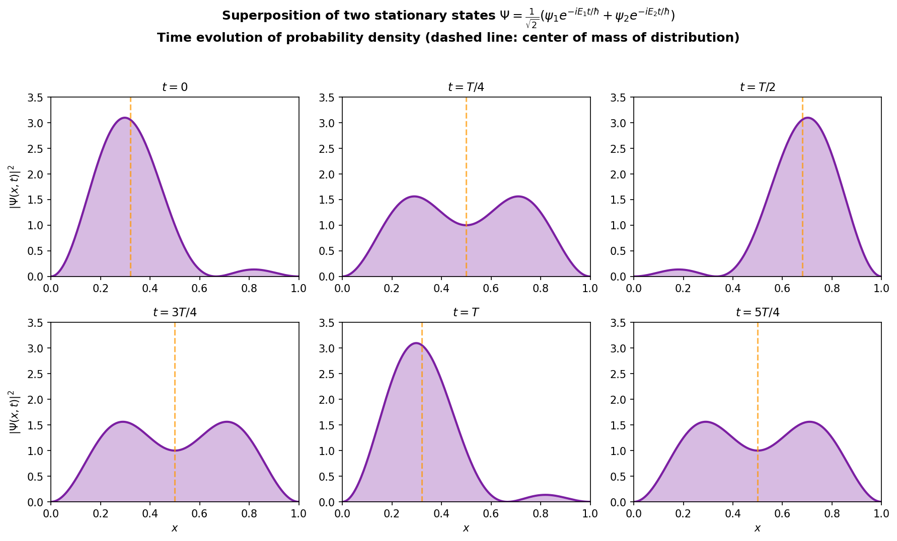
Fig. 7.4: Time evolution of probability density for a superposition state. \(|\Psi(x,t)|^2\) for an equal superposition of two stationary states \(\Psi = \frac{1}{\sqrt{2}}(\psi_1 e^{-iE_1 t/\hbar} + \psi_2 e^{-iE_2 t/\hbar})\). The dashed line shows the "center of mass" of the probability distribution, which oscillates with period \(T = 2\pi\hbar/(E_2 - E_1)\).
🔵 Kai: The probability peak is oscillating! Is this the same mechanism as the Rabi oscillations in Ch. 6? So this is what it looks like in position space.
🟡 Lina: Exactly. In Ch. 6, the probability between two states oscillated, but now it's the probability of "where in position space the particle is found" that oscillates—the mechanism is exactly the same.
🔵 Kai: Then if you superpose three or more energy eigenstates, does the oscillation become more complex?
🟡 Lina: Yes. With three or more components, interference terms with different frequencies \(\omega_{21}, \omega_{31}, \omega_{32}, \ldots\) all overlap, so it's no longer simple back-and-forth motion. But the basic mechanism is the same—phase differences between different energy components generate time variation. With \(N\) components, the number of interference terms is the number of pairs—\(_NC_2 = N(N-1)/2\).
⚪ Mei: With 2 components there's 1 giving simple oscillation, with 3 there are 3 giving complex oscillation—the more components, the more rapidly the interference terms proliferate.
🟡 Lina: Right. And the structure is the same for every interference term—the frequency is determined by "the energy difference between two components"—equation (7.20)'s \(\omega_{21} = (E_2 - E_1)/\hbar\) just becomes \(\omega_{nm} = (E_n - E_m)/\hbar\) for any pair \((n, m)\).
🔵 Kai: But something bugs me—if the probability peak is oscillating, is the particle actually moving back and forth? Or is it just that "the probability of where you'd find it if you measured is changing"?
🟡 Lina: Sharp question. Precisely the latter. The particle isn't tracing a classical trajectory. What's happening is that the distribution of "if you measured now, the probability of finding it here is high" changes over time. Until measurement, the particle has no definite position—this is the fundamental difference from classical mechanics.
🔵 Kai: Hmm, "it's not moving" but "the probability of where you'd find it is changing"... I get it intellectually, but it still feels uncomfortable intuitively. If the probability peak oscillates left and right, you want to say "the particle is moving." So before measurement, what is the particle actually "doing"?
🟡 Lina: That question touches the deepest part of quantum mechanics. To answer honestly at this stage—quantum mechanics says nothing about "what the particle is doing before measurement." All it can say is "if you measure, you'll find it here with such-and-such probability." This discomfort is a perfectly normal reaction—Einstein felt the same way. For now, let's proceed with the attitude "it feels weird, but the calculations work." In 7.9 "Overall Summary — The Structure of the Schrödinger Equation", we'll sort out "what's deterministic and what's probabilistic" in comparison with Newton's mechanics.
🔵 Kai: ...Honestly I'm still not convinced, but "the calculations work" is strong evidence. OK, I'll put it on hold for now and focus on getting comfortable with the equation first. I'll definitely ask again later though.
✅ Comprehension Check: Does the probability density \(|\Psi(x,t)|^2\) of a stationary state \(\Psi(x,t) = \psi(x)e^{-iEt/\hbar}\) depend on time? Answer with reasoning.
Answer
It does not depend on time. \(|\Psi|^2 = |\psi(x)|^2|e^{-iEt/\hbar}|^2 = |\psi(x)|^2 \cdot 1 = |\psi(x)|^2\). The absolute value of the phase factor is always 1, so the probability density is time-independent. That's why it's called a "stationary state."
📝 Exercises:
- Substitute the separation of variables \(\Psi(x,t) = \psi(x)T(t)\) into the Schrödinger equation (7.13) and carry out the process of separating into an equation in \(x\) only and an equation in \(t\) only → Problem M-1. Derivation of the Time-Independent Schrödinger Equation via Separation of Variables
7.6 Probability Density and Probability Current — Conservation of Probability¶
🟡 Lina: The most important physical requirement on the wave function is "conservation of probability." Particles don't disappear or appear from nothing. So the total probability of finding the particle somewhere in all space must always be 1:
🔵 Kai: But \(\Psi\) changes with time, right? Does this integral really stay at 1 forever?
🟡 Lina: Good question. Let's prove it. We'll compute the time derivative of the integral. Intuitively, "the rate of change of total probability" is "the sum of the rates of change of probability density at all points"—because if the whole changes, it's because some part is changing. Let me confirm one technical point here. "Differentiating with respect to \(t\) then integrating over \(x\)" and "integrating over \(x\) then differentiating with respect to \(t\)" can't always be interchanged freely. But when the wave function approaches 0 sufficiently fast as \(x \to \pm\infty\)—a condition we'll formally require in 7.7 "Normalization and Physical Requirements on the Wave Function"—we can cut off the integration range at a sufficiently large finite interval \([-L, L]\) with barely any change in the result. For integrals over a finite interval, as long as the integrand is smooth, differentiation and integration can be freely interchanged—intuitively, since an integral is "an infinitely fine sum," "differentiating each term of the sum then adding" and "adding then differentiating" give the same thing. Note that the \(\frac{d}{dt}\) on the left is ordinary differentiation of "a function of \(t\) only remaining after integrating over \(x\)," while the \(\frac{\partial}{\partial t}\) on the right is partial differentiation of "a function depending on both \(x\) and \(t\)." That is:
First let's compute \(\frac{\partial}{\partial t}|\Psi|^2\). Since \(|\Psi|^2 = \Psi^*\Psi\):
⚪ Mei: The product rule for differentiation.
🟡 Lina: We want to extract \(\frac{\partial\Psi}{\partial t}\) from the Schrödinger equation (7.13). Just divide both sides by \(i\hbar\)—dividing by \(i\hbar\) is the same as multiplying by \(\frac{1}{i\hbar} = \frac{-i}{\hbar}\). Why? Because multiplying numerator and denominator of \(\frac{1}{i}\) by \(-i\) gives \(\frac{1}{i} = \frac{-i}{-i^2} = \frac{-i}{1} = -i\). The left side becomes \(i\hbar\frac{\partial\Psi}{\partial t} \cdot \frac{1}{i\hbar} = \frac{\partial\Psi}{\partial t}\). The right side:
🔵 Kai: Multiplying by \(-\frac{i}{\hbar}\) makes the \(i\hbar\) disappear. \(-\frac{i}{\hbar} \cdot (-\frac{\hbar^2}{2m})\): minus times minus is plus, \(\hbar\) cancels, giving \(\frac{i\hbar}{2m}\). The equation checks out.
🟡 Lina: Right. Next, take the complex conjugate of this equation. Since \(V\) is real, \(V^* = V\), and \(i^* = -i\):
🔵 Kai: All the signs of \(i\) get flipped.
🟡 Lina: Substituting these into equation (7.23):
The terms containing \(V\) cancel:
🔵 Kai: Oh, the potential \(V\) terms cancelled!
🟡 Lina: Right. Because \(V\) is real, the \(V\)-containing terms from the \(\Psi^*\) equation and the \(\Psi\) equation cancel exactly. This is an important point—probability conservation depends on \(V\) being real. If \(V\) were complex, the cancellation would break down and probability wouldn't be conserved.
⚪ Mei: So the condition for probability conservation is directly linked to the property of the potential (being real).
🟡 Lina: Exactly. Now look closely at the right side of equation (7.26). There are two terms: \(\Psi^*\frac{\partial^2\Psi}{\partial x^2}\) and \(\frac{\partial^2\Psi^*}{\partial x^2}\Psi\). Let's try to rewrite this in the form of "a derivative with respect to \(x\)." Expanding \(\frac{\partial}{\partial x}\left(\Psi^*\frac{\partial\Psi}{\partial x}\right)\) using the product rule:
Similarly:
Taking the difference of these two, the \(\frac{\partial\Psi^*}{\partial x}\frac{\partial\Psi}{\partial x}\) terms cancel:
This is exactly what remains on the right side of equation (7.26). Combining the left side gives \(\frac{\partial}{\partial x}\left(\Psi^*\frac{\partial\Psi}{\partial x} - \frac{\partial\Psi^*}{\partial x}\Psi\right)\), so:
🔵 Kai: I see—we tried "can we write this in the form of a derivative with respect to \(x\)?" and it worked out.
🟡 Lina: Right. The reason we look for this form is that if we can write \(\frac{\partial\rho}{\partial t} = \frac{\partial(\text{something})}{\partial x}\), then integrating over all space makes the right side depend only on boundary values, which lets us show probability conservation. The physical motivation comes first.
⚪ Mei: We're reverse-engineering "what form do we want to arrange it into" from the goal.
🟡 Lina: Looking at the right side of equation (7.27), it's in the form of the \(x\)-derivative of \(\frac{i\hbar}{2m}\left(\Psi^*\frac{\partial\Psi}{\partial x} - \frac{\partial\Psi^*}{\partial x}\Psi\right)\). That is, \(\frac{\partial}{\partial t}|\Psi|^2 = \frac{\partial}{\partial x}(\text{something})\). This has the same form as mass conservation in fluid dynamics—"time change of density = spatial change of flow." In fluid dynamics we write \(\frac{\partial\rho}{\partial t} + \frac{\partial j}{\partial x} = 0\) and call \(j\) the "current." To match this form, we want to write the right side as \(-\frac{\partial j}{\partial x}\). Equation (7.27) is \(\frac{\partial}{\partial t}|\Psi|^2 = \frac{\partial}{\partial x}\left[\frac{i\hbar}{2m}(\cdots)\right]\), so to get \(\frac{\partial}{\partial t}|\Psi|^2 = -\frac{\partial j}{\partial x}\) we define \(j = -\frac{i\hbar}{2m}(\cdots)\). Note that \(-\frac{i\hbar}{2m}\) can also be written as \(\frac{\hbar}{2mi}\). To verify: \(\frac{1}{i} = \frac{1}{i}\cdot\frac{-i}{-i} = \frac{-i}{1} = -i\), so \(\frac{\hbar}{2mi} = \frac{\hbar}{2m}\cdot\frac{1}{i} = \frac{\hbar}{2m}\cdot(-i) = -\frac{i\hbar}{2m}\). Since different textbooks use different notations, here we adopt the \(\frac{\hbar}{2mi}\) form to define the probability current density \(j(x,t)\):
With this definition, equation (7.27) becomes the clean form \(\frac{\partial}{\partial t}|\Psi|^2 = -\frac{\partial j}{\partial x}\). Check it—the right side of (7.27) is \(\frac{\partial}{\partial x}\left[\frac{i\hbar}{2m}(\cdots)\right]\), and \(j = -\frac{i\hbar}{2m}(\cdots)\), so the right side \(= \frac{\partial}{\partial x}\left[-j\right] = -\frac{\partial j}{\partial x}\).
🔵 Kai: I see—the sign of \(\frac{i\hbar}{2m}\) and \(j\) are opposite, so differentiating with respect to \(x\) gives \(-\frac{\partial j}{\partial x}\).
🟡 Lina: Exactly. The physical meaning of the minus sign is "where probability density increases, probability current is flowing in"—we define it so that inflow and density increase have the same sign.
🔵 Kai: Is there some physical image for the definition of probability current \(j\) in equation (7.28)? Just looking at the formula, it seems complex...
🟡 Lina: Good question. Physically, since \(\hat{p} = -i\hbar\frac{\partial}{\partial x}\), we have \(\frac{\hat{p}}{m} = \frac{-i\hbar}{m}\frac{\partial}{\partial x}\), which is the quantum version of classical mechanics' "velocity = momentum/mass." An alternative way to write it is \(j = \text{Re}\left[\Psi^*\frac{-i\hbar}{m}\frac{\partial\Psi}{\partial x}\right]\). Note here that \(\frac{\partial}{\partial x}\) means "differentiate the function immediately to its right," and \(\Psi^*\) is already to the left of the derivative so it doesn't get differentiated—so the order is: compute \(\Psi^* \times \frac{-i\hbar}{m}\frac{\partial\Psi}{\partial x}\), then take the real part. To verify: setting \(z = \Psi^*\frac{-i\hbar}{m}\frac{\partial\Psi}{\partial x}\) and using \(\text{Re}(z) = \frac{z + z^*}{2}\), we get \(z^* = \Psi\frac{i\hbar}{m}\frac{\partial\Psi^*}{\partial x}\) (the sign of \(i\) flips, and \(\Psi\) and \(\Psi^*\) swap), so \(\frac{z + z^*}{2} = \frac{-i\hbar}{2m}\!\left(\Psi^*\frac{\partial\Psi}{\partial x} - \frac{\partial\Psi^*}{\partial x}\Psi\right) = \frac{\hbar}{2mi}\!\left(\Psi^*\frac{\partial\Psi}{\partial x} - \frac{\partial\Psi^*}{\partial x}\Psi\right)\), matching equation (7.28)—verify this with your own hands in problem Problem M-3. Calculation of Probability Current Density. So this is "the real part of sandwiching the velocity operator \(\hat{v} = \hat{p}/m\) between \(\Psi^*\) and \(\Psi\)," interpretable as the quantum version of the classical "density × velocity = current."
🔵 Kai: So the classical "current = density × velocity" becomes a form using operators in quantum mechanics.
🟡 Lina: Right. Therefore equation (7.27) can be written as \(\frac{\partial}{\partial t}|\Psi|^2 = -\frac{\partial j}{\partial x}\). Rearranging:
🟡 Lina: This form of equation is called the continuity equation. It has exactly the same structure as the equation expressing "mass doesn't appear or disappear" in fluid dynamics. The probability density \(\rho = |\Psi|^2\) represents "density of probability" and \(j\) represents "flow of probability." Probability neither appears nor disappears—meaning probability is locally conserved. See Fig. 7.5 "Probability current and probability conservation" for the image of a wave packet moving while total probability is preserved. Note that in general a wave packet spreads (disperses) over time as it moves, but the total probability \(\int|\Psi|^2 dx = 1\) is always preserved—that's the meaning of the continuity equation.
⚪ Mei: Probability conservation is expressed in the same form as mass conservation in fluids. Even if the shape changes, the "total amount" doesn't change.
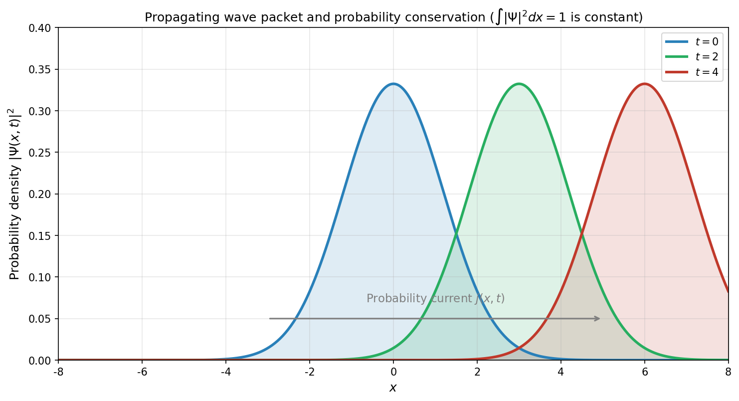
Fig. 7.5: Probability current and probability conservation. A wave packet moving over time (schematic diagram neglecting dispersion here). The shape of the wave packet generally spreads over time, but the integral over all space \(\int|\Psi|^2 dx = 1\) is always preserved. The probability current \(j(x,t)\) represents the "flow of probability."
🔵 Kai: And the integral over all space stays constant?
🟡 Lina: Integrating both sides of the continuity equation (7.29) over \(x\) from \(-\infty\) to \(+\infty\), the left side gives \(\frac{d}{dt}\int|\Psi|^2 dx\), and the right side gives \(-\int_{-\infty}^{+\infty}\frac{\partial j}{\partial x}\,dx\). We use the fundamental theorem of calculus from high school: \(\int_a^b f'(x)dx = f(b) - f(a)\). Here \(\int_{-\infty}^{+\infty}\left(-\frac{\partial j}{\partial x}\right)dx\), thinking of \(-j\) as "the function before differentiating with respect to \(x\)":
Here \(\int_{-\infty}^{+\infty}\frac{\partial j}{\partial x}dx = [j]_{-\infty}^{+\infty} = j(+\infty) - j(-\infty)\) is the fundamental theorem of calculus itself. With the overall minus sign, \(-(j(+\infty) - j(-\infty)) = j(-\infty) - j(+\infty)\) flips the sign.
Physically meaningful wave functions approach 0 sufficiently fast as \(x \to \pm\infty\), so \(j(\pm\infty, t) = 0\) and the right side is 0:
🔵 Kai: Amazing! Once normalized, it stays normalized forever.
🟡 Lina: This is an important result demonstrating the internal consistency of the Schrödinger equation. If this property didn't hold, the probability interpretation itself would break down.
⚪ Mei: So probability conservation emerges from the mathematical structure of the equation. It wasn't imposed as an extra condition after the fact.
🟡 Lina: Right. More precisely, in Ch. 6 we confirmed probability conservation (\(|C_1|^2 + |C_2|^2 = 1\) being time-independent). This is the position-representation expression of that. The "length" of the state vector—in position representation, \(\int|\Psi|^2\,dx\)—is preserved under time evolution. This property is called unitarity.
✅ Comprehension Check: In the proof of probability conservation (equation 7.26), why do the terms containing the potential \(V(x)\) cancel? What would happen if \(V(x)\) were complex?
Answer
Because \(V(x)\) is real, \(\Psi^*(-\frac{i}{\hbar}V\Psi)\) and \((\frac{i}{\hbar}V\Psi^*)\Psi\) cancel exactly. If \(V(x)\) were complex, the cancellation would be incomplete and probability would not be conserved. That is, the potential being real is a necessary condition for probability conservation.
✅ Comprehension Check: Explain the physical meaning of the continuity equation (7.29) in terms of the relationship between "the increase or decrease of probability within a region" and "probability current."
Answer
The rate of change of probability within the interval \([a, b]\), \(P_{ab} = \int_a^b |\Psi|^2 dx\), is \(\frac{dP_{ab}}{dt} = j(a,t) - j(b,t)\). That is, probability within the interval increases only when the probability current flowing in from the left end is greater than that flowing out from the right end. Probability never "springs from nowhere"—it always flows in from adjacent regions.
📝 Exercises:
- Calculate the probability current density \(j\) for a plane wave \(\Psi = Ae^{i(kx - \omega t)}\) and compare with the classical "particle current" \(\rho v\) (\(\rho\) is probability density, \(v\) is velocity) → Problem M-3. Calculation of Probability Current Density
7.7 Normalization and Physical Requirements on the Wave Function¶
🟡 Lina: From the discussion of probability conservation, let's summarize the physical conditions that wave functions must satisfy.
Normalization Condition¶
🟡 Lina: First, the most basic condition:
This is the mathematical expression of "the particle must be somewhere."
🔵 Kai: What if a \(\Psi\) obtained by solving the Schrödinger equation doesn't integrate to 1?
🟡 Lina: Since it's a linear equation, multiplying a solution by a constant gives another solution. If the integral gives a finite value \(N\), replacing \(\Psi\) with \(\Psi/\sqrt{N}\) normalizes it. However, if the integral diverges (goes to infinity), normalization is impossible—such a function doesn't represent a physical state.
⚪ Mei: The plane wave \(e^{ikx}\) is exactly that case. \(\int_{-\infty}^{+\infty}|e^{ikx}|^2 dx = \int_{-\infty}^{+\infty}1\,dx = \infty\).
🟡 Lina: Right. A plane wave is an idealization of "a state with definite momentum"—physically it needs to be used as part of a wave packet superposition. Mathematically it's a convenient tool, but it can't be normalized on its own.
Continuity and Smoothness¶
🟡 Lina: Next, the smoothness conditions the wave function must satisfy:
- \(\Psi(x,t)\) must be continuous
- \(\frac{\partial\Psi}{\partial x}\) must also be continuous (when the potential is finite)
🔵 Kai: Why does it have to be smooth?
🟡 Lina: Two reasons. First, the probability current \(j\) (equation 7.28) contains \(\frac{\partial\Psi}{\partial x}\), so if it's discontinuous, the probability current can't be defined. Second, the right side of the Schrödinger equation contains \(\frac{\partial^2\Psi}{\partial x^2}\), so if \(\frac{\partial\Psi}{\partial x}\) is discontinuous, the second derivative can't be defined.
⚪ Mei: So for the Schrödinger equation to make sense, the wave function must be at least twice differentiable.
🟡 Lina: However, there's an exception. At points where the potential jumps to infinity (infinitely high walls), continuity of \(\frac{\partial\Psi}{\partial x}\) is not required. We'll see this concretely in Ch. 9.
Summary of Boundary Conditions¶
🟡 Lina: Let me summarize the conditions for physically allowed wave functions:
Table 7.2: List of boundary conditions for wave functions
| Condition | Mathematical expression | Physical reason |
|---|---|---|
| Normalizable | $\int | \Psi |
| Continuous | No discontinuities in \(\Psi\) | Probability density is uniquely defined |
| Smooth connection | \(\partial\Psi/\partial x\) continuous | Probability current is conserved |
| Zero at infinity | \(\Psi \to 0\) (\(x \to \pm\infty\)) | Particle is not at infinity |
🔵 Kai: These conditions generate energy quantization, right? Not "any \(E\) has a solution," but only those \(E\) satisfying these conditions are allowed.
🟡 Lina: Exactly! That's the heart of quantum mechanics. When we solve the square well potential and harmonic oscillator concretely in Ch. 9, we'll see how boundary conditions select the allowed energies.
✅ Comprehension Check: Of the four physical requirements on the wave function (normalizable, continuous, smooth connection, zero at infinity), which are responsible for producing energy quantization?
Answer
All of these conditions combined produce energy quantization. In particular, solutions satisfying both normalizability (\(\Psi \to 0\) at \(x \to \pm\infty\)) and continuity/smoothness conditions simultaneously exist not for arbitrary energies \(E\), but only for specific discrete values \(E_n\). The boundary conditions restrict which solutions exist, thereby selecting the allowed energies.
✅ Comprehension Check: Is the wave function \(\Psi(x) = A\) (constant) normalizable? State your reasoning.
Answer
Not normalizable. \(\int_{-\infty}^{+\infty}|A|^2 dx = |A|^2 \cdot \infty = \infty\), which diverges.
7.8 Feynman's Perspective — From Lattice to Continuous Space¶
🟡 Lina: Here I'll introduce another perspective on where the Schrödinger equation comes from. It's the beautiful approach Feynman showed in The Feynman Lectures on Physics.
🔵 Kai: Is it different from the derivation we just did?
🟡 Lina: Earlier we took the approach of "reading off the equation from the properties of de Broglie waves." Feynman's approach is "to derive the Schrödinger equation as the limit of taking lattice spacing to zero in the equation for electrons on a crystal lattice."
🟡 Lina: Consider a line of atoms spaced at interval \(b\). Write the position of the \(n\)-th atom as \(x_n = nb\). Write the probability amplitude for the electron to be at the \(n\)-th atom at time \(t\) as \(C(x_n)\)—the same thing as \(C_1, C_2\) from Ch. 6, but since there are infinitely many atoms, it's more convenient to label by position \(x_n\) rather than number \(n\) when taking the continuous limit later (it really depends on \(t\) too, but I'll write it concisely). In Ch. 6's ammonia molecule, two configurations exchanged with amplitude \(A\). With the same reasoning, let the probability amplitude for the electron to "hop" to a neighboring atom be \(A\) (\(A > 0\)). Then the time evolution of the amplitude at the \(n\)-th atom, following the same structure as \(i\hbar\frac{dC_i}{dt} = \sum_j H_{ij}C_j\) from Ch. 6, is:
- Diagonal element \(H_{nn} = E_0\) (energy when staying at the \(n\)-th atom without hopping): \(E_0 C(x_n)\)
- Coupling to right neighbor \((n+1)\) (off-diagonal element \(H_{n,n+1} = -A\), same structure as \(H_{12} = -A\) in Ch. 6): \(-A C(x_n + b)\)
- Coupling to left neighbor \((n-1)\) (off-diagonal element \(H_{n,n-1} = -A\)): \(-A C(x_n - b)\)
Combining these:
🔵 Kai: This is a generalization of the ammonia maser from Ch. 6! Instead of two states, there are infinitely many atoms.
🟡 Lina: I've illustrated this structure in Fig. 7.6 "Feynman's lattice model", so check it out.
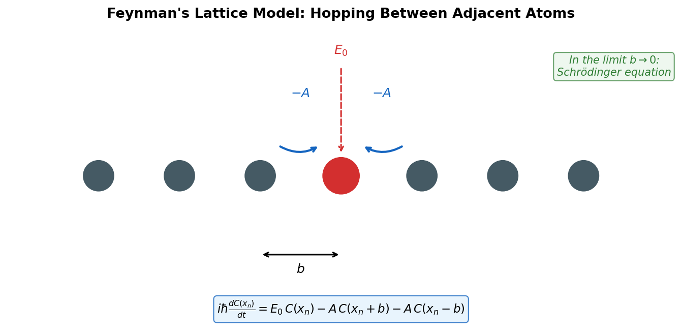
Fig. 7.6: Feynman's lattice model. An electron on atoms spaced at interval \(b\). The amplitude at the \(n\)-th atom evolves in time through its own energy \(E_0\) and coupling \(-A\) to left and right neighboring atoms. In the limit \(b \to 0\) of lattice spacing, the continuous-space Schrödinger equation emerges.
🔵 Kai: Why is the sign negative for "hopping in" from a neighbor?
🟡 Lina: Recall the ammonia molecule equations from Ch. 6. There we had \(i\hbar\frac{dC_1}{dt} = H_{11}C_1 + H_{12}C_2\) with \(H_{12} = -A\) (\(A > 0\)). As a result, the eigenvalues split into \(E_0 + A\) and \(E_0 - A\), with the lower energy being \(E_0 - A\)—meaning coupling lowered the energy. The key point is that "the minus in \(-A\) is just a convention." If we fix \(A > 0\) and write the off-diagonal element as \(-A\), then coupling results in energy lower than \(E_0\) (\(E_0 - A < E_0\)). If we wrote \(+A\), energy would increase instead, contradicting the physics that "being able to hop to a neighbor makes things more stable." In high school chemistry you learned that "forming a covalent bond stabilizes things (lowers energy)," right? Same thing here—an electron that can hop to a neighbor has lower energy than one confined to a single atom. That's why we write \(-A\).
⚪ Mei: So the sign convention reflects the physics that "coupling lowers the energy."
🟡 Lina: Right. Let me rearrange the right side a bit. The goal is to bring the "difference from neighbors" into the form of a second derivative. The second derivative \(\frac{d^2f}{dx^2}\) represents "the curvature of a function," but on a discrete lattice it's approximated by "the deviation of the middle value from the average of both neighbors." Specifically, \(f''(x) \approx \frac{f(x+b) - 2f(x) + f(x-b)}{b^2}\)—looking at the numerator, it has the form "add both neighbor values, subtract twice the middle." Flipping the sign: \(2f(x) - f(x+b) - f(x-b) \approx -b^2 f''(x)\). To create this form in the right side of equation (7.33), we add \(+2AC(x_n) - 2AC(x_n) = 0\):
We split these 5 terms into 2 groups. Pair \(E_0 C(x_n)\) with \(-2AC(x_n)\) to get \((E_0 - 2A)C(x_n)\). From the remaining \(+2AC(x_n) - AC(x_n+b) - AC(x_n-b)\), factor out \(A\) to get \(A[2C(x_n) - C(x_n+b) - C(x_n-b)]\). Combined:
🔵 Kai: Ah, you combined \(E_0 C - 2AC\) into \((E_0 - 2A)C\) and put the rest in brackets. The bracket content is "twice the middle value minus both neighbors"—and this turns into a second derivative?
🟡 Lina: Exactly! That's precisely the point. But first, let me address one thing. \((E_0 - 2A)\) is merely a constant energy shift—just as you could freely choose the reference point for potential energy in high school physics, where you place the "zero" of energy doesn't affect the physics.
🔵 Kai: Wait, but \(E_0\) is the energy of staying at an atom, and \(A\) is the strength of hopping coupling, right? Is it OK to just eliminate them?
🟡 Lina: Good check. What matters here is only "energy differences." Adding or subtracting a constant from everything just adds a common phase factor \(e^{-i(E_0-2A)t/\hbar}\) in the time evolution equation, which doesn't affect the probability density \(|\Psi|^2\)—the same logic as "overall phase doesn't affect physics" from Ch. 6. So we choose the energy origin such that \(E_0 - 2A = 0\) and eliminate it. Then only the bracket content remains. Now let me answer Kai's question. 🟡 Lina: If \(C(x)\) is a smooth function, we can approximate it using a Taylor expansion. A Taylor expansion is a method of expressing the value of a function at nearby points using "derivative coefficients at that point." Intuitively, writing \(f(x+b)\) as a power series in \(b\) gives \(f(x+b) = f(x) + bf'(x) + \frac{b^2}{2}f''(x) + \cdots\) (\(f'\) is shorthand for first derivative, \(f''\) for second). The first term is "the original value," the second is "slope × displacement" as a first-order correction, and the third is "the second-order correction due to curvature." The smaller \(b\) is, the more rapidly the higher-order terms shrink, improving accuracy.
🔵 Kai: Concretely, what does that mean?
🟡 Lina: Try it with \(f(x) = x^2\). \(f(x+b) = (x+b)^2 = x^2 + 2xb + b^2\). On the other hand, applying the Taylor expansion formula: \(f(x) + bf'(x) + \frac{b^2}{2}f''(x) = x^2 + b(2x) + \frac{b^2}{2}(2) = x^2 + 2xb + b^2\). They match perfectly. You might wonder where the \(\frac{1}{2}\) in \(\frac{b^2}{2}\) comes from—looking at the \(x^2\) example, expanding \((x+b)^2\) gives a coefficient of \(1\) for the \(b^2\) term. Meanwhile \(f''(x) = 2\), so multiplying \(f''\) by \(\frac{b^2}{2}\) gives \(\frac{b^2}{2} \times 2 = b^2\), correctly reproducing it. So the \(\frac{1}{2}\) is "the coefficient that cancels the extra 2 that comes from differentiating twice." In general, the coefficient of the \(n\)-th order term is \(\frac{1}{n!}\) (\(n\) factorial, \(n! = n \times (n-1) \times \cdots \times 2 \times 1\)). See Appendix B for details. For general functions it's an approximation, but for small \(b\) it's an extremely good one.
🔵 Kai: I see—for \(x^2\) it matches exactly, but for general functions it's an approximation that gets better as \(b\) gets smaller.
🟡 Lina: Using this:
Adding these two, the first-order terms (\(+b\frac{\partial C}{\partial x}\) and \(-b\frac{\partial C}{\partial x}\)) cancel:
⚪ Mei: Because we added \(+b\) and \(-b\), the first-order terms (\(\pm b\frac{\partial C}{\partial x}\)) cancelled, leaving only the second derivative term.
🔵 Kai: Are we going to replace \(Ab^2\) with something?
🔵 Kai: But why only hopping to "the nearest atom"? Can't it hop directly to one two sites away?
🟡 Lina: Good question. In principle, hopping to the next-nearest neighbor is possible, but its amplitude is much smaller than the nearest-neighbor amplitude \(A\). Quantum tunneling weakens exponentially with distance, so considering only the nearest neighbors is a good approximation. This is called the "nearest-neighbor approximation."
🟡 Lina: Now, substituting equation (7.35) into equation (7.34) (after setting \(E_0 - 2A = 0\)):
For this to match the free-particle Schrödinger equation (7.11), we need \(Ab^2 = \hbar^2/(2m)\). Conversely, the effective mass of the particle is determined from the lattice model parameters \(A\) and \(b\) as \(m = \hbar^2/(2Ab^2)\). Thus:
🔵 Kai: It's the free-particle Schrödinger equation! It emerges as the continuous limit of the discrete lattice equation. But if \(Ab^2 = \hbar^2/(2m)\), does \(A\) keep growing as \(b \to 0\)?
⚪ Mei: Since \(A = \hbar^2/(2mb^2)\), when \(b\) halves, \(A\) quadruples—indeed \(A \to \infty\) as \(b \to 0\).
🟡 Lina: Right. As the lattice spacing \(b\) decreases, the hopping amplitude \(A\) to the neighbor increases—which makes sense if you think "the closer the neighbor, the easier it is to hop." With \(A \propto 1/b^2\) increasing as \(b \to 0\), the motion of a particle with finite mass \(m\) in continuous space is reproduced. What about the case with a potential?
🟡 Lina: In the lattice model, the energy \(E_0\) varies from site to site depending on position—that is, replacing \(E_0 \to E_0 + V(x_n)\), the \(V(x)\Psi\) term naturally appears in the continuous limit. But as Feynman himself emphasized, this isn't a rigorous "derivation" but rather a "clue" giving physical motivation for the Schrödinger equation. Ultimately, the Schrödinger equation is accepted as a hypothesis consistent with experiment. But it's a beautiful perspective showing that the quantum mechanics of discrete systems (what we learned in Chapters 4–6) connects naturally to quantum mechanics in continuous space.
⚪ Mei: The story of finite dimensions from Chapters 5–6 and the continuous-space story of this chapter are connected in a single line through the lattice model.
✅ Comprehension Check: In Feynman's lattice model, why must \(Ab^2\) be kept constant when taking the limit \(b \to 0\)?
Answer
\(Ab^2 = \hbar^2/(2m)\) is the quantity that determines the particle's mass. If only \(A\) were held fixed as \(b \to 0\), then \(Ab^2 \to 0\) and the kinetic energy term would vanish. To obtain a physically meaningful continuous limit, \(A\) must grow proportionally to \(b^{-2}\) while \(b \to 0\).
7.9 Overall Summary — The Structure of the Schrödinger Equation¶
🟡 Lina: Let's organize the framework introduced in this chapter. Mei, could you summarize?
⚪ Mei: I'll try.
Table 7.3: Summary of fundamental concepts of the Schrödinger equation
| Concept | Mathematical expression | Physical meaning |
|---|---|---|
| Wave function | \(\Psi(x,t) = \langle x\vert\phi(t)\rangle\) | Probability amplitude for finding the particle at position \(x\) |
| Probability density | \(\rho(x,t) = \lvert\Psi(x,t)\rvert^2\) | Finding probability per unit length |
| Time evolution | \(i\hbar\frac{\partial\Psi}{\partial t} = \hat{H}\Psi\) | Schrödinger equation |
| Hamiltonian | \(\hat{H} = -\frac{\hbar^2}{2m}\frac{\partial^2}{\partial x^2} + V(x)\) | Energy operator |
| Momentum operator | \(\hat{p} = -i\hbar\frac{\partial}{\partial x}\) | Operator that extracts momentum |
| Stationary states | \(\hat{H}\psi_n = E_n\psi_n\) | Energy eigenstates |
| Probability conservation | \(\frac{\partial\rho}{\partial t} + \frac{\partial j}{\partial x} = 0\) | Continuity equation |
🔵 Kai: Laying it all out like this, I'm starting to see the structure. Is it the same kind of structure as \(F = ma\) in Newton's mechanics—"solve the equation to find something"?
🟡 Lina: Great observation. That's exactly right, and let me lay out the comparison in a table. One thing I want you to notice is the difference in "order of differentiation." Newton's equation of motion contains the second time derivative (acceleration), so you need two initial conditions: position and velocity. The Schrödinger equation, on the other hand, contains only the first time derivative, so the initial condition \(\Psi(x,0)\) alone is sufficient—that alone determines the future.
Table 7.4: Structural comparison of Newton's mechanics and quantum mechanics
| Newton's mechanics | Quantum mechanics | |
|---|---|---|
| Fundamental equation | \(F = ma\) (Newton's equation of motion) | \(i\hbar\frac{\partial\Psi}{\partial t} = \hat{H}\Psi\) (Schrödinger equation) |
| What we solve for | Position \(x(t)\) | Wave function \(\Psi(x,t)\) |
| Meaning | Definite trajectory of particle | Distribution of probability amplitudes |
| Initial conditions | Position \(x(0)\) and velocity \(v(0)\) | Wave function \(\Psi(x,0)\) |
| Measurement outcome | Deterministic (definite position obtained) | Probabilistic (\(\|\Psi\|^2\) gives probability density) |
| Time evolution | Deterministic (\(x(t)\) uniquely determined from initial conditions) | Deterministic (\(\Psi(x,t)\) uniquely determined from initial conditions) ※Measurement outcomes are probabilistic |
| Order of differentiation | Second order in time | First order in time |
🔵 Kai: But \(\Psi\) doesn't tell us "the particle's actual position" like \(x(t)\) does, right? I asked this in 7.5 "Stationary States and the Time-Independent Schrödinger Equation" too, but I want to confirm it again within the overall picture.
🟡 Lina: Right. Newton's \(x(t)\) gives the particle's "definite position." On the other hand, \(\Psi(x,t)\) is a probability amplitude, giving "the distribution of probability for finding the particle." Where the particle will be found in any individual measurement cannot be predicted.
🔵 Kai: The table says "time evolution is deterministic" but measurement outcomes are probabilistic... so is quantum mechanics deterministic or probabilistic? Which is it?
🟡 Lina: Interestingly, it's only half deterministic. Given the initial condition \(\Psi(x, 0)\), the Schrödinger equation uniquely determines \(\Psi(x,t)\) at all future times. In that sense, the time evolution of the wave function is deterministic. But "where will the particle be at the next measurement" can only be predicted probabilistically.
⚪ Mei: So what's deterministic is the time evolution of \(\Psi\), not individual measurement outcomes.
🔵 Kai: But the time evolution of \(\Psi\) is deterministic while measurement makes it probabilistic—where's the "boundary" between those? What physically happens during measurement?
🟡 Lina: That's one of the deepest problems in quantum mechanics, called the "measurement problem." It's beyond the scope of this textbook, but it's an important question. For now, let's accept that the Schrödinger equation is the best hypothesis consistent with experiment—it hasn't been falsified at any scale from atoms, molecules, and solids to elementary particles since its proposal in 1926—and move forward.
🔵 Kai: So the Schrödinger equation describes "time evolution between measurements," and "measurement itself" is a separate story. Honestly I still feel uneasy but... Let me ask the reverse then: if you don't measure, does \(\Psi\) keep evolving deterministically forever? As long as you don't measure, "probability" never appears?
🟡 Lina: That's correct. As long as no measurement is made, the wave function evolves completely deterministically according to the Schrödinger equation. "Probability" only shows its face at the moment of measurement. This strangeness lies at the very heart of quantum mechanics. For now, let's first master using the equation and get a feel for what can be predicted and what cannot.
🔵 Kai: In Newton's mechanics, solving \(F = ma\) tells you "where the particle will be next instant," but solving the Schrödinger equation doesn't tell you "where the particle will be found at the next measurement"—even though both are "solving a fundamental equation," the nature of what you get is fundamentally different. But I suppose I won't understand until I actually use it.
⚪ Mei: To summarize—what the Schrödinger equation describes is time evolution "between measurements," which is deterministic. But at the moment of measurement, results come out probabilistically according to \(|\Psi|^2\)—it's a two-stage structure.
✅ Comprehension Check: Are "quantum mechanics is deterministic" and "quantum mechanics is probabilistic" contradictory? Explain how they coexist.
Answer
The time evolution of the wave function (Schrödinger equation) is deterministic—the future wave function is uniquely determined from the initial condition. However, what is obtained from the wave function is the probability distribution of measurement outcomes, and individual measurement results can only be predicted probabilistically. They coexist in the form "evolution of the state is deterministic, but measurement outcomes are probabilistic."
📝 Exercises:
- Verify that the Gaussian wave packet \(\Psi(x, 0) = \left(\frac{2a}{\pi}\right)^{1/4}e^{-ax^2}\) satisfies the normalization condition \(\int_{-\infty}^{+\infty}|\Psi|^2 dx = 1\) (you may use the Gaussian integral \(\int_{-\infty}^{+\infty}e^{-\alpha x^2}dx = \sqrt{\pi/\alpha}\)) → Problem A-1. Time Evolution of a Gaussian Wave Packet and Wave Packet Spreading
Preview of Next Chapter¶
🟡 Lina: In this chapter, the "stage setting" of the Schrödinger equation is complete. But we're still missing important tools.
🔵 Kai: What's missing?
🟡 Lina: How to compute "the expectation value of position" and "the expectation value of momentum." And the quantitative expression of the fact that position and momentum cannot be determined simultaneously with perfect accuracy—the uncertainty principle. In Ch. 8, we'll develop methods for calculating expectation values of operators, and from the "commutation relation" \([\hat{x}, \hat{p}] = i\hbar\) between the position operator \(\hat{x}\) and momentum operator \(\hat{p}\), we'll derive Heisenberg's uncertainty principle \(\Delta x\,\Delta p \geq \hbar/2\).
⚪ Mei: Methods for extracting "averages" and "spreads" from probability amplitudes. Looking forward to it.
🟡 Lina: Furthermore, we'll also prove Ehrenfest's theorem—that expectation values obey classical equations of motion. We'll see how the bridge between quantum mechanics and classical mechanics works.
References¶
- D. J. Griffiths, Introduction to Quantum Mechanics, 3rd ed., Cambridge University Press (2018), Ch.1: Statistical interpretation of the wave function, time invariance of normalization, introduction of operators
- 広江克彦『趣味で量子力学』, Ch.5: Concrete solutions of the 1D Schrödinger equation, boundary conditions for the square well potential
- 清水明『新版 量子論の基礎』, Ch.5: Time evolution of closed systems, unitary evolution and probability conservation, time evolution of energy eigenstates
- R. P. Feynman, R. B. Leighton, M. Sands, The Feynman Lectures on Physics, Vol. III, Ch.16: "The Dependence of Amplitudes on Position" — Transition from lattice model to continuous-space Schrödinger equation, probability density interpretation of the wave function
- J. J. Sakurai, J. Napolitano, Modern Quantum Mechanics, 3rd ed., Cambridge University Press (2021), Ch.2: Time evolution operator, Schrödinger and Heisenberg pictures, expansion in energy eigenkets
Feedback on this page
Let us know if something was unclear, incorrect, or could be improved.