Chapter 4: Why Do Successful Models Break Down? — The Crisis of Classical Physics
Story so far: In Chapters 1–3, we examined three successful models: Newtonian mechanics (gravity), Maxwell's electromagnetism (unification of electricity, magnetism, and light), and Boltzmann's statistical mechanics (entropy). Each possessed astonishing predictive power, and by the end of the 19th century, some believed that "physics is nearly complete."
Goals of this chapter
- Relive how classical physics—thought to be "nearly complete" at the end of the 19th century—was broken by three experimental facts: the ultraviolet catastrophe in black-body radiation, the photoelectric effect, and the perihelion precession of Mercury
- Internalize the essence of science that "no matter how successful a model is, it must be revised if it contradicts experiment," and obtain a complete map showing which chapters in Part II and beyond resolve each question
4.1 "Physics Is Nearly Complete"?
🟡 Lina: At the end of the 19th century, some physicists believed that "all the fundamental laws have been found. All that remains is improving precision beyond the decimal point."
🔵 Kai: Were they really that confident?
🟡 Lina: Newtonian mechanics could explain everything from planets to cannonballs. Maxwell's electromagnetism unified electricity, magnetism, and light. Thermodynamics explained thermal phenomena through entropy. Indeed, it appeared that nearly all phenomena could be explained.
🔵 Kai: "Nearly" means there were still phenomena that couldn't be explained?
🟡 Lina: Exactly. The British physicist Lord Kelvin reportedly said around 1900 that "there are only two clouds remaining in the sky of physics." One was the problem of the speed of light (experiments attempting to detect the medium "ether" that supposedly carried light had failed, leaving the mechanism of light speed unexplained), and the other was the problem of thermal radiation (the spectrum of black-body radiation couldn't be explained). However, these "mere two clouds" turned out to be harbingers of an enormous storm that would fundamentally rewrite the entire picture of physics. We'll address the speed of light problem in Ch. 5; in this chapter, we'll start from the thermal radiation problem and examine three crises that classical physics faced.
🔵 Kai: Something that appeared to be a small problem was actually fatal... But why couldn't physicists at the time recognize this? With three pillars working so well, wouldn't it be hard to take "just two clouds" seriously?
🟡 Lina: Good question. That's a very important point in the philosophy of science. All models are hypotheses, and no matter how successful they are, they can be overturned by a single experimental fact. The property that "it can be shown wrong by experiment"—this is called falsifiability. Falsifiability is both the strength of science and its severity.
🔵 Kai: So it's not "proven correct," but rather "no errors have been found yet"?
🟡 Lina: Exactly. No matter how successful a model is, there's always the possibility that the next experiment will overturn it. That's the attitude of science.
Philosophy of science note: The optimism that "physics is nearly complete" resulted from confusing models with "truth." A model is merely "the best hypothesis that has not yet been refuted by experiment." When we forget this attitude, our response is delayed when a crisis arrives. Develop the ability to judge for yourself.
✅ Comprehension Check: What are the three models that served as the basis for believing "physics is nearly complete" at the end of the 19th century?
Answer
Newtonian mechanics, Maxwell's electromagnetism, and thermodynamics (statistical mechanics).
4.2 The First Crisis: The Ultraviolet Catastrophe of Black-Body Radiation
Setting Up the Problem
🟡 Lina: Heated objects emit light. When iron is heated, it glows red; heated further, it glows white. An idealized object that "absorbs all incoming light and emits radiation determined solely by its temperature" is called a black body. A good approximation is a completely enclosed cavity with a small hole—light entering through the hole bounces off the interior walls multiple times and is almost entirely absorbed. When we try to calculate the spectrum of "thermal radiation" emitted by this black body using classical physics—what the intensity is at each frequency—
🔵 Kai: What happens?
🟡 Lina: At high frequencies (the ultraviolet side)—high frequency means short wavelength (recall the relation \(c = \lambda\nu\))—the radiated energy becomes infinite. This is called the ultraviolet catastrophe. It "diverges" on the "ultraviolet" side, hence the name. Look at Fig. 4.1 "Conceptual diagram of the black-body radiation spectrum"—you can see at a glance how much the classical theory prediction and experimental data disagree.
%%{init: {"theme": "default", "themeCSS": ".edgePath .path, .flowchart-link { stroke-width: 2px !important; }"}}%%
---
config:
  theme: base
  themeVariables:
    xyChart:
      plotColorPalette: "#e53935, #1e88e5"
---
xychart-beta
    title "Black-Body Radiation Spectrum (Conceptual Diagram)"
    x-axis "Frequency ν →" [0, 1, 2, 3, 4, 5, 6, 7, 8]
    y-axis "Radiation Energy Density u(ν) →"
    line "Experiment (Planck)" [0, 2, 5, 7, 6, 4, 2, 1, 0.5]
    line "Classical Theory (Rayleigh-Jeans)" [0, 0.5, 2, 4.5, 8, 12.5, 18, 24.5, 32]
Fig. 4.1: Conceptual diagram of the black-body radiation spectrum
The classical theory (Rayleigh-Jeans) increases without bound at high frequencies (ultraviolet catastrophe). Experimental data turns over and decreases at high frequencies. Planck derived a spectrum matching experiment by assuming energy quantization \(E = h\nu\).
Note: Frequency \(\nu\) and wavelength \(\lambda\) are related by \(c = \lambda\nu\). High frequency = short wavelength. The name "ultraviolet catastrophe" comes from the divergence on the "ultraviolet (short wavelength = high frequency) side."
Derivation of the Rayleigh-Jeans Formula
🟡 Lina: Let's trace through the equations to see why classical physics fails. Consider electromagnetic waves confined in a sealed box (cavity). Let the length of one side of the box be \(L\). We'll use the tools from statistical mechanics that we learned in Ch. 3.
🔵 Kai: Statistical mechanics comes up here?
🟡 Lina: Yes. First, Step 1: Counting modes. We consider what shapes electromagnetic waves can take inside the box. The walls of the box are metallic, so the electric field must be zero at the wall positions—metal contains many freely moving electrons, and if there were an electric field at the wall surface, electrons would be pulled by that field and instantly rearrange, redistributing charge to cancel the original field. Therefore, the electric field is always maintained at zero on a metal surface. This is the flip side of "metals conduct electricity"—precisely because electrons can move freely, they maintain zero electric field at the surface. With the electric field at zero at the walls, the walls become "nodes" of the wave. The wave then bounces back and forth between the walls, and the rightward-traveling and leftward-traveling waves superpose to form a standing wave—a wave that oscillates in place without propagating. Think of a guitar string—both ends of the string are fixed (they're nodes), so only waves whose half-wavelengths fit an integer number of times within the string length can exist.
🔵 Kai: The fundamental mode, second harmonic, third harmonic... right.
🟡 Lina: Exactly. The condition for exactly \(n_x\) half-wavelengths \(\lambda_x/2\) to fit within the box length \(L\) is:
Here we define the wave number \(k\) as \(k = 2\pi/\lambda\). \(1/\lambda\) represents "how many wave cycles fit in one meter," and \(k\) is that multiplied by \(2\pi\). It's a quantity representing the spatial "fineness" of the wave. Substituting \(\lambda_x = 2L/n_x\):
Similarly \(k_y = n_y\pi/L\), \(k_z = n_z\pi/L\) (\(n_x, n_y, n_z\) are positive integers).
🔵 Kai: It's the three-dimensional version of standing waves on a guitar string.
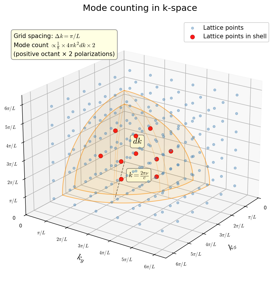
Fig. 4.2: Standing wave modes in a box and wave number space. The allowed electromagnetic wave modes in a cubic cavity of side \(L\) correspond to lattice points in wave number space. The detailed counting method (the \(1/8\) factor and polarization factor of 2) is explained in the text.
🟡 Lina: Exactly. Look at Fig. 4.2 "Standing wave modes in a box and wave number space". Since the relationship between the magnitude of the wave number \(k = |\boldsymbol{k}|\) and frequency \(\nu\) is \(k = 2\pi\nu/c\), we want to count the number of modes in the frequency range from \(\nu\) to \(\nu + d\nu\).
Here's the picture. Consider a "wave number space" with \(k_x, k_y, k_z\) as the three axes. The allowed modes correspond to lattice points at \((k_x, k_y, k_z) = (n_x\pi/L,\; n_y\pi/L,\; n_z\pi/L)\). The spacing between lattice points in each direction is \(\pi/L\), so the volume per lattice point is \((\pi/L)^3\).
🔵 Kai: It's like a three-dimensional grid.
🟡 Lina: Right. Since standing waves have the form \(\sin(n_x\pi x/L)\), changing \(n_x\) to \(-n_x\) gives \(\sin(-n_x\pi x/L) = -\sin(n_x\pi x/L)\)—only the overall sign flips, and the "shape" of the wave (where the nodes and antinodes are) remains the same. The overall sign of the amplitude has no physical meaning (since wave intensity is determined by the square of the amplitude), so \(n_x\) and \(-n_x\) represent the same mode. Therefore, to count independent modes, we only take positive integers. This means lattice points exist only in the "first octant" of wave number space (\(k_x > 0,\; k_y > 0,\; k_z > 0\), one of the 8 octants). So we count only \(1/8\) of all space. The wave number range corresponding to frequencies from \(\nu\) to \(\nu + d\nu\) is a spherical shell from radius \(k\) to \(k + dk\). The volume of this shell is \(4\pi k^2\,dk\). The number of lattice points within \(1/8\) of this shell is:
Here the factor of 2 reflects the fact that electromagnetic waves have two polarizations—two directions in which the electric field can oscillate. As we learned in Ch. 2, electromagnetic waves are transverse waves (waves whose oscillation direction is perpendicular to the propagation direction), and the electric field oscillates in a plane perpendicular to the propagation direction. For example, if light is traveling in the \(z\) direction, the electric field oscillates in the \(xy\) plane. There are only two independent directions within this plane—the \(x\) direction and the \(y\) direction—oscillation at 45° can be expressed as "equal parts of \(x\)-direction oscillation and \(y\)-direction oscillation added together," so it's not a new independent direction. It's exactly like how any vector in a plane can be decomposed into \(x\) and \(y\) components. So for each wave number, there are two modes differing only in polarization.
⚪ Mei: So \((\pi/L)^3\) is the volume per lattice point in wave number space, and we divide the shell volume by it to get the number of lattice points. The \(1/8\) is for counting only positive integers, and the \(\times 2\) is for the polarization degrees of freedom.
🟡 Lina: Right. Substituting \(k = 2\pi\nu/c\) and converting with \(dk = (2\pi/c)\,d\nu\):
Let's organize this step by step. First the prefactors: \(2 \times \frac{1}{8} \times 4\pi = \pi\). Next the \(k^2\,dk\) part: \((2\pi\nu/c)^2 \cdot (2\pi/c)\,d\nu = \frac{4\pi^2\nu^2}{c^2} \cdot \frac{2\pi}{c}\,d\nu = \frac{8\pi^3\nu^2}{c^3}\,d\nu\). The denominator is \((\pi/L)^3 = \pi^3/L^3\). Putting it all together:
(Verify that \(\pi \times 8\pi^3 / \pi^3 = 8\pi\).)
Dividing by the box volume \(V = L^3\), we get the mode density per unit volume \(g(\nu)\):
🔵 Kai: Up to this point, it's just geometric counting—no physical assumptions have been introduced?
🟡 Lina: Essentially yes. The only inputs are the boundary condition "electric field is zero at the walls" and the property "electromagnetic waves are transverse with 2 polarization directions." No statistical mechanical assumptions have been used yet.
🔵 Kai: I understand the factor of 2 from polarization. But if light were a longitudinal wave, there would be no polarization degree of freedom and no factor of 2?
🟡 Lina: Exactly. For longitudinal waves like sound waves, there's only one oscillation direction (along the propagation direction), so there would be no factor of 2. The fact that electromagnetic waves are transverse is essential here.
🟡 Lina: Now, everything up to this point is a purely geometric result determined only by the box shape and electromagnetic boundary conditions. The problem lies in the next step—how much energy to assign to each mode.
Step 2: Applying the equipartition theorem. According to Boltzmann's statistical mechanics from Ch. 3, in thermal equilibrium each degree of freedom receives an average energy of \(\frac{1}{2}k_B T\). A single mode of electromagnetic waves oscillates with the electric and magnetic fields alternately exchanging energy. This is mathematically the same structure as a mass on a spring—what physicists call a harmonic oscillator—alternating between kinetic energy and potential energy.
🔵 Kai: What does "mathematically the same structure" mean, specifically?
🟡 Lina: When you pull a mass on a spring and release it, the restoring force (the spring trying to return to its natural length) makes the mass oscillate. This restoring force is "proportional to the displacement"—that's Hooke's law. The equation of motion is \(m\ddot{x} = -\kappa x\), meaning oscillation driven by a "restoring force proportional to displacement" (\(\ddot{x}\) is shorthand notation for the second time derivative of position \(x\), \(d^2x/dt^2\). The spring constant is often written \(k\) in high school, but here I'll write \(\kappa\) (kappa) to avoid confusion with the wave number \(k\)). Each mode of the electromagnetic wave, when derived from Maxwell's equations, gives an electric field amplitude \(\mathcal{E}(t)\) that obeys an equation of the same form: \(\ddot{\mathcal{E}} = -\omega^2 \mathcal{E}\) (I'll write the electric field amplitude as \(\mathcal{E}\) to distinguish it from energy \(E\)).
🔵 Kai: The same form as the spring equation... but why does an electromagnetic wave obey the same equation as a spring?
🟡 Lina: Think of it intuitively like this. A standing wave can be written as the product of a "spatial shape" and a "temporal oscillation"—for example, \(\sin(k_x x)\sin(k_y y)\sin(k_z z) \times \mathcal{E}(t)\). The spatial shape is fixed by the wall boundary conditions, so only the time part \(\mathcal{E}(t)\) moves freely.
🔵 Kai: So the spatial shape is a fixed "template," and only the time-direction oscillation is free to move?
🟡 Lina: Exactly. When you substitute this form into the wave equation \(\nabla^2 f = \frac{1}{c^2}\frac{\partial^2 f}{\partial t^2}\), differentiating the spatial part produces \(-k^2\). The reason is that differentiating \(\sin(k_x x)\) twice with respect to \(x\) gives \(-k_x^2 \sin(k_x x)\) (differentiating \(\sin\) gives \(\cos\), differentiating again gives back \(-\sin\), and each time \(k_x\) comes out front). The same applies for \(y\) and \(z\) directions, so applying \(\nabla^2 = \partial^2/\partial x^2 + \partial^2/\partial y^2 + \partial^2/\partial z^2\) multiplies the whole thing by \(-(k_x^2 + k_y^2 + k_z^2) = -k^2\). The time part must satisfy \(\ddot{\mathcal{E}} = -c^2 k^2 \mathcal{E} = -\omega^2 \mathcal{E}\) (where \(\omega = ck\)). This is exactly the same form as the spring equation, and the solutions are \(\sin(\omega t)\) or \(\cos(\omega t)\). Here \(\omega = 2\pi\nu\) is the angular frequency—the frequency \(\nu\) (oscillations per second) multiplied by \(2\pi\), a convenient quantity for writing equations. Since the form of the equation is the same, the energy structure is also the same—it splits into a "term corresponding to the speed of oscillation" and a "term corresponding to the magnitude of oscillation."
⚪ Mei: So each standing wave mode in the box is mathematically equivalent to a spring, and the equipartition theorem applies directly.
🟡 Lina: Exactly. For a spring, there's kinetic energy \(\frac{1}{2}mv^2\) and potential energy \(\frac{1}{2}\kappa x^2\). Recall the equipartition theorem from Ch. 3—"\(\frac{1}{2}k_BT\) per degree of freedom." Here "degree of freedom" means independent quadratic terms appearing in the energy expression. The spring's energy has one \(v^2\) term and one \(x^2\) term, totaling 2 quadratic terms. So there are 2 degrees of freedom, each receiving \(\frac{1}{2}k_BT\). A spring has one \(v^2\) term and one \(x^2\) term, so it receives a total of \(\frac{1}{2}k_BT + \frac{1}{2}k_BT = k_BT\). An electromagnetic wave mode similarly possesses two quadratic terms: electric field energy (proportional to the square of the amplitude—corresponding to the spring's \(\frac{1}{2}\kappa x^2\)) and magnetic field energy (proportional to the square of the magnetic field amplitude—corresponding to the spring's \(\frac{1}{2}mv^2\)). Just as with a spring, where maximum displacement corresponds to zero velocity (maximum potential energy, zero kinetic energy), in electromagnetic waves when the electric field is maximum the magnetic field is zero, and when the magnetic field is maximum the electric field is zero—the two alternately exchange energy while oscillating. So the average energy per mode is:
⚪ Mei: Each mode receives a uniform energy of \(k_B T\).
🟡 Lina: Multiplying this by the mode density gives the radiation energy density per unit volume per unit frequency \(u(\nu, T)\):
This is the Rayleigh-Jeans formula.
🔵 Kai: Since it's proportional to \(\nu^2\), the energy density keeps increasing as frequency increases...!
🟡 Lina: If we integrate over all frequencies:
The integral diverges. The total energy of the electromagnetic field in the box is infinite—this is the ultraviolet catastrophe.
Why Classical Theory Breaks Down
🔵 Kai: But the mode counting itself is correct, right? Where was the mistake?
🟡 Lina: The heart of the problem lies in the equipartition theorem's assignment of a uniform \(k_B T\) to each mode.
🔵 Kai: So the number of modes increases as frequency goes up, but the energy per mode doesn't decrease, leading to divergence?
🟡 Lina: Sharp observation. High-frequency modes are infinite in number (\(g(\nu) \propto \nu^2\) keeps growing). If you assign \(k_B T\) to each, the total naturally becomes infinite. Classical physics has no mechanism to "suppress energy allocation to high-frequency modes."
🔵 Kai: In experiments, radiation decreases at high frequencies, but the classical theory has no brake for that.
Planck's Quantum Hypothesis
🟡 Lina: In 1900, Planck introduced a revolutionary hypothesis to solve this problem:
The energy of a mode with frequency \(\nu\) is not continuous, but can only take integer multiples of \(h\nu\).
Here \(h = 6.626 \times 10^{-34}\;\mathrm{J \cdot s}\) is the Planck constant.
🔵 Kai: Energy becomes "discrete"...? How does that prevent the ultraviolet catastrophe?
🟡 Lina: Let's compare how energy is distributed differently in classical and quantum theories—look at Fig. 4.3 "Energy quantization".
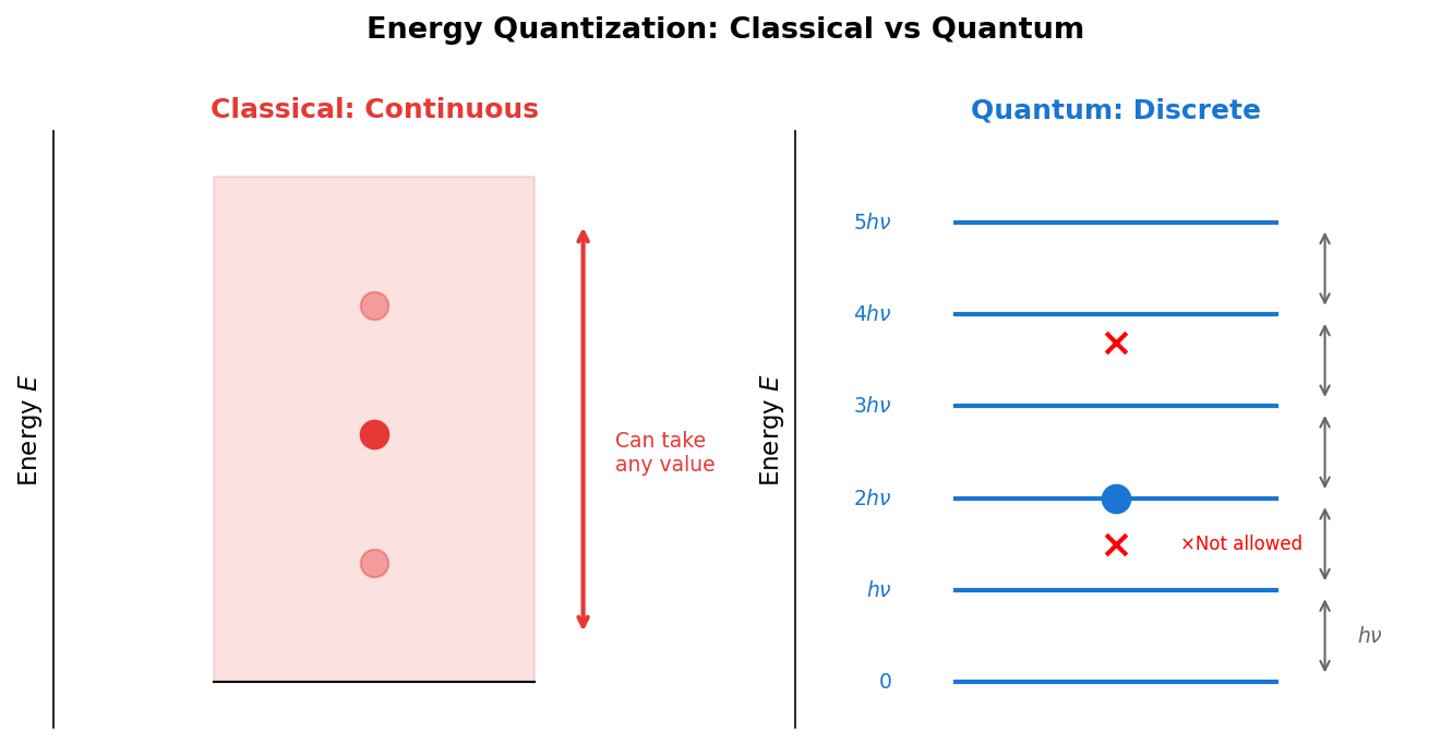
Fig. 4.3: Energy quantization. In classical theory (left), energy can take any continuous value. In quantum theory (right), energy can only take integer multiples of \(h\nu\), and intermediate values are not allowed.
🔵 Kai: I understand it becomes discrete, but just from that, I still don't see intuitively why the high-frequency side gets suppressed...
🟡 Lina: Let's recalculate the average energy per mode under this assumption. Recall the Boltzmann distribution from Ch. 3. In thermal equilibrium at temperature \(T\), the probability of being in a state with energy \(E_n\) is proportional to \(e^{-E_n/k_B T}\). To find the actual probability, we normalize by dividing by the sum of \(e^{-E_n/k_BT}\) over all states (the denominator). The average energy is the sum of "energy of each state × its probability":
Setting \(x = h\nu/k_BT\), each term in the denominator can be written as \(e^{-nh\nu/k_BT} = (e^{-h\nu/k_BT})^n = (e^{-x})^n\). This is an infinite geometric series with first term \(1\) (when \(n=0\), \((e^{-x})^0 = 1\)) and common ratio \(r = e^{-x}\) (since \(x > 0\), \(0 < r < 1\)), so using the formula \(\sum_{n=0}^{\infty} r^n = 1/(1-r)\) learned in high school:
🔵 Kai: The denominator sums up neatly as a geometric series. What about the numerator?
🟡 Lina: For the numerator series, factoring out \(h\nu\) as a constant gives \(h\nu \sum_{n=0}^{\infty} n\,e^{-nx}\). Directly computing the remaining \(\sum n\,e^{-nx}\) is difficult, but there's a clever technique. What we want is a "series with \(n\) multiplied in." Here we shift our thinking—instead of "multiplying in \(n\) ourselves," we look for "an operation that produces \(n\) naturally." Now, differentiating \(e^{-nx}\) with respect to \(x\) gives \(-n\,e^{-nx}\)—since \(-nx\) is in the exponent, differentiating brings \(-n\) down in front (just like differentiating \(e^{ax}\) gives \(a\,e^{ax}\)). So just by differentiating, \(n\) appears out front. Therefore, if we differentiate each term of the denominator series \(\sum e^{-nx}\) we just found with respect to \(x\) and add them up (for a finite sum, "derivative of the sum = sum of the derivatives" obviously holds), we automatically get the series with \(n\) multiplied in. Specifically, differentiating each term of \(\sum_{n=0}^{\infty} e^{-nx}\) with respect to \(x\):
So differentiating the entire series gives \(\sum(-n)e^{-nx}\). Flipping the sign gives \(\sum n\,e^{-nx}\):
⚪ Mei: So just by differentiating a known result, we get a new series. Clever technique.
🟡 Lina: Here we differentiate \(f(x) = (1-e^{-x})^{-1}\). Setting \(u = 1-e^{-x}\), the derivative of \(e^{-x}\) is \(-e^{-x}\), so \(du/dx = 0 - (-e^{-x}) = e^{-x}\). By the chain rule \(df/dx = (df/du)(du/dx)\):
Therefore:
🔵 Kai: I see—differentiating each term brings \(-n\) out front, so differentiating the sum of the series directly gives us \(\sum n\,e^{-nx}\). But is it really okay to differentiate infinitely many terms one by one and add them up?
🟡 Lina: Good question. First think about a finite sum. For example, differentiating \(S_3(x) = 1 + e^{-x} + e^{-2x} + e^{-3x}\) with respect to \(x\) gives \(S_3'(x) = 0 + (-1)e^{-x} + (-2)e^{-2x} + (-3)e^{-3x}\)—you just differentiate each term and add. The same works as \(N\) grows larger. Since \(e^{-nx}\) approaches zero rapidly as \(n\) increases, the contribution from distant terms becomes smaller and smaller. So the finite sum result carries over directly to the infinite sum. Rigorously, there are mathematical conditions for "being allowed to differentiate infinitely many terms simultaneously," but intuitively you can think "if the tail terms approach zero fast enough, it's fine." Series that decay exponentially, like ours, satisfy this condition perfectly. In physics, we frequently use the technique of "differentiating a known result to obtain a new result."
Therefore, the numerator is \(h\nu \cdot \frac{e^{-x}}{(1-e^{-x})^2}\) and the denominator is \(\frac{1}{1-e^{-x}}\). The average energy is numerator ÷ denominator:
(In the last equality, one factor of \((1-e^{-x})\) in the denominator cancels with the \((1-e^{-x})\) in the numerator.)
Multiplying numerator and denominator by \(e^{x}\) (numerator: \(e^{-x} \times e^x = 1\), denominator: \((1-e^{-x}) \times e^x = e^x - 1\)):
🔵 Kai: The classical \(k_B T\) has been replaced by \(\dfrac{h\nu}{e^{h\nu/k_BT} - 1}\)! But does this really eliminate the ultraviolet catastrophe?
🟡 Lina: Multiplying this by the mode density gives the Planck radiation formula:
Low-Frequency and High-Frequency Limits
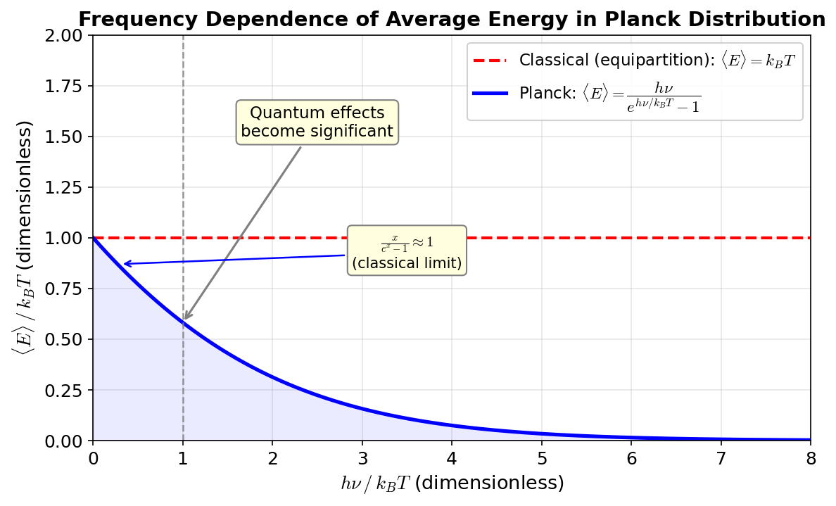
Fig. 4.4: Average energy in the Planck distribution. Average energy per mode. In classical theory (equipartition), it's uniformly \(k_BT\), but with Planck's quantum hypothesis it decays exponentially at high frequencies.
🟡 Lina: Look at Fig. 4.4 "Average energy in the Planck distribution". Let's verify that this formula is consistent with classical theory.
Low-frequency limit (\(h\nu \ll k_BT\)): Taylor expanding the exponential gives \(e^{h\nu/k_BT} \approx 1 + h\nu/k_BT\), so:
This matches the Rayleigh-Jeans formula. Classical theory was a correct approximation at low frequencies.
🔵 Kai: Oh, it properly contains the classical theory! What about the high-frequency side?
🟡 Lina: High-frequency limit (\(h\nu \gg k_BT\)): Since \(e^{h\nu/k_BT} \gg 1\):
It decays exponentially. This is the "brake" that prevents the ultraviolet catastrophe. Physically, when \(h\nu\) becomes larger than \(k_BT\), the energy of a single quantum is too large compared to the thermal energy, making it impossible to excite that mode. So radiation on the high-frequency side is suppressed.
⚪ Mei: So at low frequencies, the energy per quantum is small and the system behaves classically, while at high frequencies the energy per quantum is too large and the mode is "frozen out." The crossover occurs around \(h\nu \sim k_BT\).
🟡 Lina: Exactly. Planck's formula gives a finite value when integrated over all frequencies:
(This integral can be evaluated by the substitution \(x = h\nu/k_BT\), and the result is finite.) This is consistent with the Stefan-Boltzmann law (see Ch. 3).
📝 Exercises:
- Confirming the ultraviolet catastrophe by integrating the Rayleigh-Jeans law → Problem B-1. Verification of the Ultraviolet Catastrophe
✅ Comprehension Check: What is the ultraviolet catastrophe?
Answer
The problem that when calculating the black-body radiation spectrum with classical theory, the radiation energy diverges to infinity at high frequencies (the ultraviolet side).
✅ Comprehension Check: What hypothesis did Planck introduce to solve this problem, and what is the formula?
Answer
The hypothesis that energy takes discrete values rather than continuous ones. The formula is \(E = nh\nu\) (\(h\) is Planck's constant, \(\nu\) is frequency, \(n\) is a non-negative integer). The energy per quantum is \(E = h\nu\).
✅ Comprehension Check: Show, using a limiting operation on the formula, that Planck's radiation formula reduces to the Rayleigh-Jeans formula at low frequencies.
Answer
When \(h\nu \ll k_BT\), \(e^{h\nu/k_BT} \approx 1 + h\nu/k_BT\), so \(h\nu/(e^{h\nu/k_BT}-1) \approx k_BT\). Substituting this gives \(u(\nu,T) \approx (8\pi\nu^2/c^3)k_BT\), which matches the Rayleigh-Jeans formula.
4.3 The Second Crisis: The Photoelectric Effect
Predictions of Classical Wave Theory vs. Experiment
🟡 Lina: When light shines on a metal, electrons are ejected—the photoelectric effect. In classical wave theory, the energy of light is proportional to the square of the amplitude (i.e., intensity), so it predicts:
- Making the light stronger increases the energy of the ejected electrons
- Light of any frequency can knock out electrons if it's strong enough
- For weak light, it takes time for electrons to accumulate energy
🔵 Kai: The experimental results are different?
🟡 Lina: Completely different. What experiments showed was:
- The maximum energy of ejected electrons depends only on the frequency of light, not on intensity
- Unless the frequency exceeds a certain threshold \(\nu_0\), no electrons are ejected no matter how strong the light
- If the light exceeds the threshold, electrons are ejected instantly no matter how weak the light
⚪ Mei: The classical prediction contradicts experiment on all three points. Organizing this gives Table 4.1 "Photoelectric effect: Classical wave theory predictions vs".
Table 4.1: Photoelectric effect: Classical wave theory predictions vs. experimental facts
| Property | Classical wave theory prediction | Experimental fact |
|---|---|---|
| What determines energy | Light intensity (amplitude squared) | Light frequency |
| Threshold frequency | None (anything works if strong enough) | Exists (\(\nu < \nu_0\) doesn't work) |
| Timing of electron emission | Weak light requires accumulation time | Emitted instantly even with weak light |
✅ Comprehension Check: Name one point where classical wave theory predictions and experimental results contradict each other regarding the photoelectric effect.
Answer
Example: Classical theory predicts that stronger light increases electron energy, but experiments show the maximum kinetic energy of ejected electrons depends only on light frequency and is independent of intensity. (Other contradictions include the existence of a threshold frequency and the instantaneous emission of electrons even with weak light.)
Einstein's Light Quantum Hypothesis and Derivation
🟡 Lina: In 1905, Einstein pushed Planck's quantum hypothesis further. Planck said "the energy of wall oscillators is discrete," but Einstein claimed that light itself is a collection of particles (light quanta, later called photons) each with energy \(h\nu\).
A single light quantum collides with a single electron in the metal. For the electron to escape from the metal, it must overcome the binding energy \(W\) inside the metal (the work function). Writing energy conservation:
Look at Fig. 4.5 "Experimental setup and light quantum model of the photoelectric effect". It shows one light quantum delivering energy to one electron.
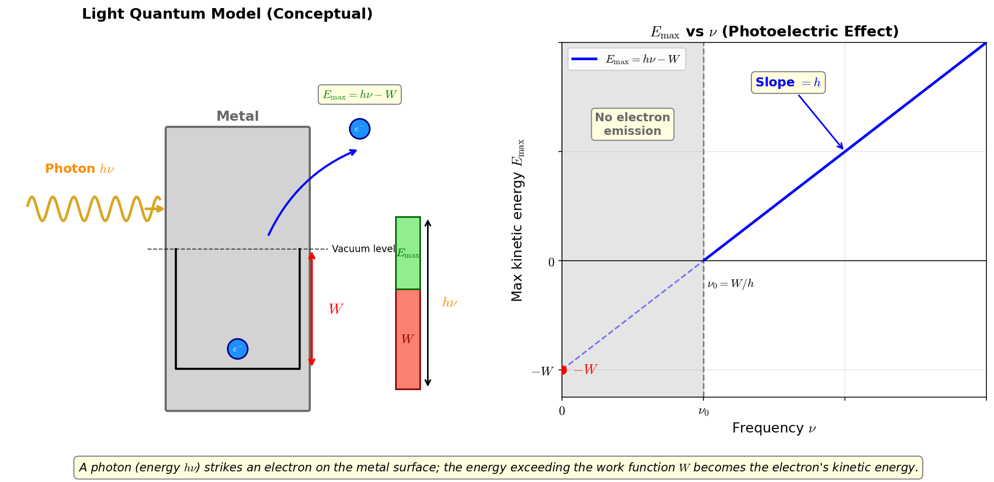
Fig. 4.5: Experimental setup and light quantum model of the photoelectric effect. A light quantum (energy \(h\nu\)) strikes an electron on the metal surface, and the energy exceeding the work function \(W\) becomes the electron's kinetic energy.
The maximum kinetic energy \(E_{\text{max}}\) of the ejected electron corresponds to the case where the electron is near the metal surface and can escape with minimal energy:
🔵 Kai: So simple...! Just the light quantum's energy minus the work function.
🟡 Lina: This formula explains all the experimental facts.
Derivation of the threshold frequency: For an electron to escape, we need \(E_{\text{max}} \geq 0\):
No electrons are ejected unless the frequency exceeds \(\nu_0 = W/h\). This is the threshold frequency.
Explanation of intensity dependence: Increasing the light intensity increases the number of light quanta. However, the energy per quantum \(h\nu\) doesn't change. So the number of ejected electrons increases, but the maximum energy per electron remains unchanged.
🔵 Kai: Stronger light = more particles, but the punch of each particle is the same.
🟡 Lina: Nice analogy. To put it in more everyday terms—think of hail. Whether a car hood gets dented depends not on the total amount of hail, but on the size of each individual hailstone.
⚪ Mei: I see. Light intensity corresponds to the total amount of hail, and the energy of one light quantum corresponds to the size of a single hailstone.
🟡 Lina: Exactly. Plotting \(E_{\text{max}}\) as a function of \(\nu\) (Fig. 4.6 "Linear relationship in the photoelectric effect"):
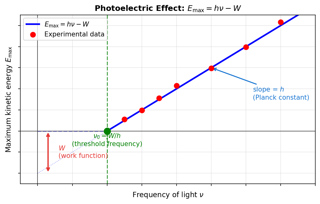
Fig. 4.6: Linear relationship in the photoelectric effect. The maximum kinetic energy \(E_{\mathrm{max}}\) of ejected electrons forms a straight line proportional to frequency \(\nu\), with the slope giving Planck's constant \(h\) and the \(\nu\)-intercept giving the threshold frequency \(\nu_0 = W/h\).
🟡 Lina: This is a straight line with slope \(h\) and intercept \(-W\). In 1916, Millikan precisely confirmed this linear relationship and independently measured the value of Planck's constant \(h\). Einstein's light quantum hypothesis was brilliantly verified.
Why Classical Theory Fails
🟡 Lina: In classical wave theory, light energy flows continuously onto the metal surface, proportional to the square of the wave amplitude. The electron slowly accumulates this energy, and once enough has built up, it escapes—that's the classical scenario.
Let's estimate the accumulation time in classical theory. Taking the electron's cross-section as atomic size \(\sim (10^{-10}\;\mathrm{m})^2 = 10^{-20}\;\mathrm{m^2}\) and assuming a typical light intensity \(I \sim 1\;\mathrm{W/m^2}\), the power received by the electron is:
The time needed to accumulate the work function energy \(W \sim 4\;\mathrm{eV} = 6.4 \times 10^{-19}\;\mathrm{J}\) is:
🔵 Kai: The calculation says it takes over a minute. But in experiments electrons come out instantly.
🟡 Lina: Experiments show electrons are emitted in less than \(10^{-9}\;\mathrm{s}\). That's a discrepancy of more than 10 orders of magnitude from the classical prediction. This isn't a precision issue—it means the mechanism is fundamentally different.
✅ Comprehension Check: When trying to explain the photoelectric effect with classical wave theory, the estimated electron emission time is about 64 seconds. How much does this deviate from experimental results?
Answer
Experiments show electrons are emitted in less than \(10^{-9}\) seconds, so there's a discrepancy of more than 10 orders of magnitude from the classical prediction. This isn't a precision issue—it shows that the classical mechanism of energy flowing in continuously is itself wrong.
The detailed quantum mechanical treatment of this problem is covered in Quantum Mechanics at Quantum Mechanics Ch. 1.
📝 Exercises:
- Calculation of the photoelectric threshold frequency → Problem B-2. Threshold Frequency of the Photoelectric Effect
✅ Comprehension Check: In the photoelectric effect, what determines whether electrons are ejected—light intensity or frequency?
Answer
Light frequency. Unless the frequency exceeds a certain threshold, no electrons are ejected no matter how much the intensity is increased.
✅ Comprehension Check: How did Einstein treat light to explain the photoelectric effect? Also, write the formula for the maximum kinetic energy of ejected electrons.
Answer
He treated light as particles (light quanta) with energy \(E = h\nu\). The maximum kinetic energy of ejected electrons is \(E_{\text{max}} = h\nu - W\) (\(W\) is the work function).
4.4 The Third Crisis: Mercury's Perihelion Precession
The Discrepancy Between Newton's Model and Observation
🟡 Lina: Mercury's orbit is an ellipse, but the ellipse itself slowly rotates (perihelion precession). Look at Fig. 4.7 "Mercury's perihelion precession". Even after calculating all the influences of other planets using Newton's model, a discrepancy of 43 arcseconds per century remains.
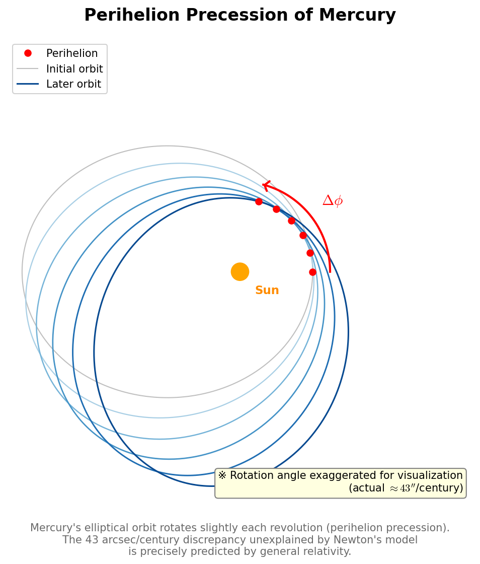
Fig. 4.7: Mercury's perihelion precession. Mercury's elliptical orbit rotates slightly with each revolution (perihelion precession). The 43 arcseconds/century discrepancy unexplainable by the Newtonian model is precisely predicted by general relativity.
🔵 Kai: 43 arcseconds is incredibly small, right?
🟡 Lina: Below "degrees" in angular units there are "arcminutes" and "arcseconds." 1 degree = 60 arcminutes, 1 arcminute = 60 arcseconds, so 1 arcsecond is \(60 \times 60 = 3600\)th of a degree. 43 arcseconds is about 0.012 degrees—the diameter of a 1-yen coin viewed at arm's length is about 1 degree, so this is about one-hundredth of that. This much over 100 years. It's certainly small. But given the precision of Newton's model, it's an unexplainable discrepancy.
Let's look at the specific numbers. Comparing the observed value of Mercury's perihelion precession with calculated values of perturbations from each planet using Newton's model (Table 4.2 "Breakdown of contributions to Mercury's perihelion precession"):
Table 4.2: Breakdown of contributions to Mercury's perihelion precession
| Cause | Perihelion precession (arcseconds/century) |
|---|---|
| Perturbation from Venus | 277.9 |
| Perturbation from Jupiter | 153.6 |
| Perturbation from Earth | 90.0 |
| Other planets | 10.5 |
| Newtonian model total | 532.0 |
| Observed value | 575.0 |
| Difference (unexplained discrepancy) | 43.0 |
⚪ Mei: Subtracting Newton's model prediction from the observed value leaves exactly 43 arcseconds.
Le Verrier's Vulcan Hypothesis
🟡 Lina: In 1859, the French astronomer Le Verrier discovered this discrepancy. He tried the same strategy we learned about in Ch. 1 with Neptune's discovery—"Could there be an unknown planet inside Mercury's orbit?"
🔵 Kai: The Neptune case was successful, right?
🟡 Lina: Yes. The discrepancy in Uranus's orbit led to predicting the existence of an unknown planet (Neptune), which was then actually discovered. Using the same logic, Le Verrier predicted a planet called "Vulcan" inside Mercury's orbit.
🔵 Kai: So, was Vulcan found?
🟡 Lina: They searched for decades but never found it. This is an important lesson. With Neptune, "the model is correct, there's an unknown element" worked. But this time, the model itself needed to be modified.
Resolution by General Relativity (Presenting the Result)
🟡 Lina: In 1915, Einstein's general theory of relativity explained this 43-arcsecond discrepancy without any additional parameters. Showing just the result:
This is the perihelion precession per orbit (in radians). Here: - \(G\): gravitational constant - \(M\): mass of the Sun - \(c\): speed of light - \(a\): semi-major axis of Mercury's orbit (the longer radius of the ellipse—corresponding to the average of the closest and farthest distances from the Sun) - \(e\): orbital eccentricity of Mercury (a dimensionless quantity representing how "squished" the ellipse is. \(e = 0\) means a perfect circle; the closer \(e\) is to 1, the more elongated the ellipse. Mercury has \(e \approx 0.206\), somewhat more elliptical among solar system planets)
🔵 Kai: Where does this formula come from?
🟡 Lina: It's derived from the Schwarzschild solution in general relativity (the geometry of spacetime around a spherically symmetric mass). The derivation requires solving the geodesic equation in curved spacetime, so I'll defer that to Ch. 6. → See General Relativity at General Relativity Ch. 10 for details.
However, we can read the "meaning" of this formula even at this stage.
🔵 Kai: The combination \(GM/c^2\) appears—what does it represent?
🟡 Lina: Good question. \(R_s = 2GM/c^2\) is called the Schwarzschild radius. Intuitively, it corresponds to the radius at which, in Newtonian mechanics, the escape velocity from the surface equals the speed of light \(c\).
🔵 Kai: Escape velocity is the speed needed for a rocket to break free from Earth's gravity, right?
🟡 Lina: Yes. It can be derived from energy conservation. Consider an object launched from the surface of a body of radius \(r\) at velocity \(v\). The kinetic energy at the surface is \(\frac{1}{2}mv^2\), and the gravitational potential energy is \(-\frac{GMm}{r}\).
🔵 Kai: Why is the potential energy negative?
🟡 Lina: Because we set infinity (where gravitational influence vanishes) as the reference zero. Since gravitational force weakens with distance and becomes completely zero at infinity, it's natural to set "no binding = zero energy" there. Closer to the body means more gravitationally bound—lower energy—hence negative. The value \(-GMm/r\) is the work (energy) \(GMm/r\) needed to move the object from distance \(r\) to infinity against the gravitational force \(F = GMm/r^2\), with a minus sign. Since the force weakens with distance, the work to reach infinity converges to a finite value (\(\int_r^\infty GMm/r'^2\,dr' = GMm/r\)—the integrand goes as \(1/r'^2\), so the antiderivative is \(-1/r'\). Unlike the high school formula for work with constant force \(F \times d\), when force varies you need integration, but just remembering the result is fine).
⚪ Mei: So setting "infinity as zero" means all bound states are negative—intuitively it's like "being in a hole."
🟡 Lina: Exactly. The condition for the velocity to be exactly zero at infinity—meaning the total energy (kinetic + potential) is exactly zero—is \(\frac{1}{2}mv^2 - \frac{GMm}{r} = 0\), i.e., \(\frac{1}{2}mv^2 = \frac{GMm}{r}\). Canceling \(m\) gives \(v = \sqrt{2GM/r}\). Setting \(v = c\) and solving for \(r\) gives \(r = 2GM/c^2 = R_s\) (the rigorous derivation requires general relativity, but the scale is correct from this estimate).
🔵 Kai: I see, so \(R_s\) is the radius where escape velocity equals the speed of light.
🟡 Lina: The \(GM/c^2\) appearing in the perihelion precession formula corresponds to \(R_s/2\). Here it serves as a yardstick measuring "how strong the relativistic gravitational effects are." The larger \(R_s\) is compared to the orbital radius, the larger the deviation from Newton's model. For the Sun, \(R_s \approx 3\;\mathrm{km}\). Compared to Mercury's orbital radius \(a \approx 5.8 \times 10^7\;\mathrm{km}\):
🔵 Kai: 5 hundred-millionths... incredibly small.
🟡 Lina: That's why the perihelion precession discrepancy is also small. But accumulated over 100 years it becomes 43 arcseconds, which was detectable by 19th-century precision astronomy. Let's substitute the numbers:
Substituting values in SI units (m, kg, s):
Computing the numerator:
Computing the denominator (\(1 - e^2 = 1 - 0.2056^2 = 1 - 0.0423 = 0.9577\)):
Therefore:
Mercury's orbital period is about 0.241 years, so the number of orbits in 100 years is \(100/0.241 \approx 415\). The cumulative effect over 100 years:
Converting to arcseconds (\(1\;\mathrm{rad} = 180°/\pi \approx 57.3°\), \(1° = 3600\;\text{arcsec}\) so \(1\;\mathrm{rad} = 57.3 \times 3600 \approx 206265\;\text{arcsec}\)):
🔵 Kai: Exactly 43 arcseconds! Amazing... And all the numbers in the formula are things already known—the Sun's mass, Mercury's orbit, etc. There's no "we adjusted this to make it fit."
🟡 Lina: Exactly. "Matching the experimental value without parameter adjustments"—that's what makes a theory's persuasiveness decisive.
⚪ Mei: The extremely small ratio \(R_s/a \sim 10^{-8}\) becomes a detectable quantity through the accumulation of 415 orbits and the conversion to angle. Even small effects can be captured by precision measurements.
🟡 Lina: This was the first quantitative success of general relativity. Einstein himself reportedly said he "couldn't sleep for several days from excitement" when he obtained this calculation result.
Model Revision vs. Parameter Addition
🔵 Kai: The same method as the Neptune case didn't work this time. What was different?
🟡 Lina: Good question. Comparing the discovery of Neptune with Mercury's perihelion precession reveals a very important point in the philosophy of science. Look at Table 4.3 "Comparison of Neptune's discovery and perihelion precession" and Fig. 4.8 "Two paths when observation conflicts with model".
Table 4.3: Comparison of Neptune's discovery and perihelion precession
| Discovery of Neptune | Mercury's perihelion precession | |
|---|---|---|
| Problem | Discrepancy in Uranus's orbit | Discrepancy in Mercury's orbit |
| Attempted solution | Assume an unknown planet | Assume an unknown planet (Vulcan) |
| Result | Success (Neptune discovered) | Failure (Vulcan doesn't exist) |
| True solution | Resolved within the model | Model itself modified (general relativity) |
%%{init: {"theme": "default", "themeCSS": ".edgePath .path, .flowchart-link { stroke-width: 2px !important; }"}}%%
flowchart TD
    A["Observation doesn't match model"] --> B{"Can it be resolved within the model?"}
    B -->|"Yes"| C["Add unknown elements<br>(parameter adjustment)"]
    B -->|"No"| D["Modify the model itself<br>(paradigm shift)"]
    C --> E["✅ Discovery of Neptune<br>Resolved within Newton's model"]
    C --> F["❌ Vulcan hypothesis<br>Didn't exist"]
    F --> D
    D --> G["✅ General relativity<br>Replaced Newton's model"]

    style E fill:#c8e6c9
    style F fill:#ffcdd2
    style G fill:#c8e6c9
Fig. 4.8: Two paths when observation conflicts with model
🟡 Lina: "When a model's predictions don't match, should we adjust parameters within the model, or modify the model itself?"—this judgment is one of the most difficult parts of science. The correct answer isn't known in advance. It gradually becomes clear through the dialogue between experiment and theory.
✅ Comprehension Check: Le Verrier tried the same strategy for Mercury's perihelion precession discrepancy as for Neptune's discovery. What was that strategy, and why did it fail this time?
Answer
The strategy of assuming an unknown planet (Vulcan) exists inside Mercury's orbit. With Neptune, the problem could be resolved by adding an unknown element within the model (Newtonian mechanics), but this time Vulcan didn't exist, making resolution within the model impossible. The true resolution required modifying the model itself (transitioning to general relativity).
📝 Exercises:
- Mercury's perihelion precession and the limits of Newton's model → Problem A-1. Mercury's Perihelion Precession and the Limits of the Newtonian Model
✅ Comprehension Check: How large is the discrepancy in Mercury's perihelion precession that Newton's model cannot explain?
Answer
43 arcseconds per century.
✅ Comprehension Check: What model explained this 43-arcsecond discrepancy without additional parameters?
Answer
Einstein's general theory of relativity (1915).
4.5 Map of Unsolved Questions
🟡 Lina: Let's organize the questions remaining from the previous 3 chapters and the new questions born in this chapter. This will be the map for Part II and beyond. First, look at the figure giving an overview of the three crises (Fig. 4.9 "Three crises of classical physics").
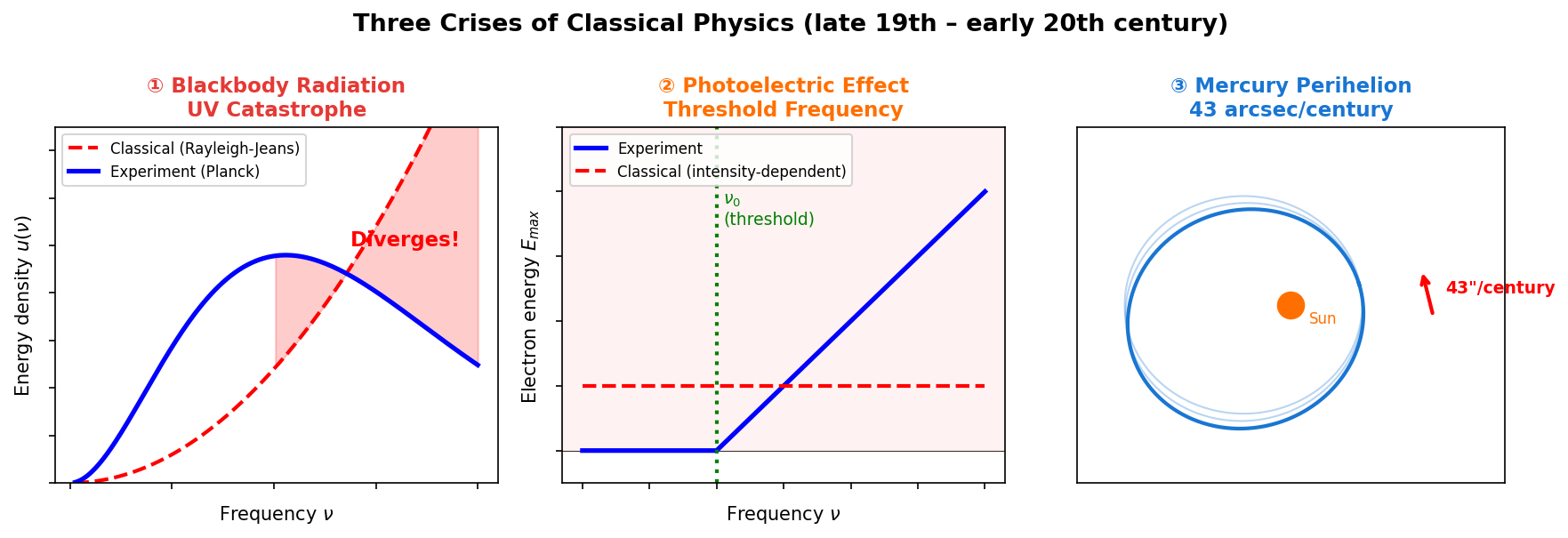
Fig. 4.9: Three crises of classical physics. ① The ultraviolet catastrophe of black-body radiation (energy density diverges at high frequencies in classical theory), ② The threshold frequency of the photoelectric effect (particle nature of light), ③ Mercury's perihelion precession (43 arcseconds/century discrepancy unexplainable by Newton's model).
⚪ Mei: Summarizing the three crises in a comparison table gives Table 4.4 "Comparison of the three crises of classical physics".
Table 4.4: Comparison of the three crises of classical physics
| Crisis | Classical prediction | Experimental fact | Theory that resolved it |
|---|---|---|---|
| Black-body radiation | Energy density diverges at high frequencies | Decreases at high frequencies | Planck's quantum hypothesis (\(E = nh\nu\)) |
| Photoelectric effect | Energy determined by light intensity | Energy determined by frequency | Einstein's light quantum hypothesis |
| Mercury's perihelion precession | All explained by planetary perturbations | 43 arcsec/century discrepancy remains | Einstein's general relativity |
🔵 Kai: It's nicely organized. But both black-body radiation and the photoelectric effect are "quantum" stories, and Mercury seems to go in a different direction.
🟡 Lina: Good observation. Organizing things, we see that the three crises each demand revolutions in different directions. Black-body radiation and the photoelectric effect suggest "discreteness of energy" and point toward quantum mechanics. Mercury's perihelion precession suggests "geometry of spacetime" and points toward general relativity. And the speed of light problem points toward special relativity. In other words, quantum mechanics changes "what is continuous and what is discrete," while relativity changes "the shape of spacetime itself"—since the targets of modification differ, they developed as separate theories.
⚪ Mei: So of the three crises, two point in the "discreteness" direction and one in the "geometry" direction, and since the targets of modification differ, they became separate theories.
Table 4.5: Unsolved questions and where they are resolved
| Question | Where it's resolved |
|---|---|
| Why is the speed of light the same for everyone? (Ch. 2) | → Ch. 5 Special Relativity |
| What is the true nature of gravity? Mercury's perihelion precession? (Ch. 1, Ch. 4) | → Ch. 6 General Relativity |
| What is the fundamental principle behind the "discreteness of energy" that produces black-body radiation and the photoelectric effect? (Discovered in Ch. 4, systematized in Ch. 7) | → Ch. 7 Quantum Mechanics |
| Making quantum mechanics and relativity compatible (revealed in Ch. 7) | → Ch. 8 Quantum Field Theory |
| Can the 4 forces be unified? (extension of Ch. 2) | → Ch. 9 The Standard Model |
| Contradiction between gravity and quantum mechanics (revealed in Ch. 6, Ch. 8) | → Part III The Quantum Gravity Problem |
| A unified theory? (revealed in Ch. 9) | → Part IV String Theory |
%%{init: {"theme": "default", "themeCSS": ".edgePath .path, .flowchart-link { stroke-width: 2px !important; }"}}%%
graph TD
    A["Three crises of classical physics<br>(Chapter 4)"] --> B["The mystery of light speed<br>Chapter 5: Special Relativity"]
    A --> C["The nature of gravity<br>Chapter 6: General Relativity"]
    A --> D["The quantum world<br>Chapter 7: Quantum Mechanics"]
    B --> E["Relativistic quantum theory<br>Chapter 8: Quantum Field Theory"]
    D --> E
    C --> F["Contradiction between gravity and quantum<br>Part III: Quantum Gravity Problem"]
    E --> F
    E --> G["Unification of forces<br>Chapter 9: The Standard Model"]
    F --> H["Attempts at unified theory<br>Part IV: String Theory"]
    G --> H

    style A fill:#ffcdd2
    style F fill:#fff9c4
    style H fill:#c8e6c9
Fig. 4.10: From the crises of classical physics to the chapter structure ahead
🔵 Kai: So this is the whole map... But if quantum mechanics and general relativity head in different directions, don't they eventually contradict each other? If both are correct but incompatible, isn't that strange?
🟡 Lina: That's precisely the core issue. Each is astonishingly correct in its own domain, but when you try to use both simultaneously, contradictions arise. "Resolution" brings new models that generate new questions. This chain continues all the way to Part V.
🔵 Kai: "Using both simultaneously"—what kind of situation specifically? Normally one is enough, right?
🟡 Lina: Good question. For example, the center of a black hole, or the first moments of the universe—situations where extremely large mass is concentrated in an extremely small region. There, gravity is strong (requiring general relativity) yet the scale is extremely small (also requiring quantum mechanics). Neither alone can describe it. We'll cover this in detail in Part III.
⚪ Mei: To make Kai's question more concrete—black-body radiation and Mercury's perihelion precession demand modifications in completely different directions. Discreteness of energy and geometry of spacetime—the targets of modification are different, yet when we try to use both simultaneously, what specific form does the contradiction take?
🟡 Lina: Good organization. When I said "contradict," to be more precise, applying quantum mechanical methods to gravity causes calculations to diverge—a problem similar to the ultraviolet catastrophe reappears in a more fundamental form. How to resolve this contradiction is the theme of Part III and beyond.
🔵 Kai: So the ultraviolet catastrophe we saw in this chapter comes back in a different form...
Philosophy of science note: The three crises vividly demonstrate the structure of science where "the breakdown of a successful model gives birth to a new model." However, note that new models are also merely hypotheses. General relativity and quantum mechanics may be replaced by even deeper models in the future. A "final theory" may not exist. Never forget the attitude of judging for yourself.
✅ Comprehension Check: In which chapter of Part II are the problems of black-body radiation and the photoelectric effect resolved?
Answer
Ch. 7 (Quantum Mechanics).
✅ Comprehension Check: In which part of this textbook is the contradiction between quantum mechanics and general relativity addressed?
Answer
Part III (The Quantum Gravity Problem).
Preview of the Next Chapter
Ch. 5「Why Is the Speed of Light Constant? — Special Relativity」 — Einstein answers the mystery of the speed of light predicted by Maxwell's equations. Special relativity, where our common sense about time and space is rewritten.
References
- Carlo Rovelli, Reality Is Not What It Seems, Ch.3: "Albert", Ch.4: "Quanta" — Historical background of black-body radiation, photoelectric effect, and quantum hypothesis
- Lee Smolin, The Trouble with Physics, Introduction — Historical context of the crises
- David Tong, Lectures on General Relativity, Ch.1: "Geodesics in Spacetime" — Mercury's perihelion precession
- Quantum Mechanics Chapter 1 "Three Crises of Classical Physics" — More detailed treatment of black-body radiation, photoelectric effect, and atomic stability
- General Relativity Chapter 10 "Is Einstein's Model More Accurate Than Newton's?" — General relativistic derivation of Mercury's perihelion precession
- Quantum Field Theory Chapter 3 "Classical Field Theory" — Lagrangian formalism and field equations
Feedback on this page
Let us know if something was unclear, incorrect, or could be improved.