Appendix D Toolkit for Loop Calculations — Dimensional Analysis, Feynman Parameters, and Wick Rotation
Story so far:
In Appendix C we organized Gaussian integrals (single-variable and multi-variable) and the algebra of Grassmann numbers and Berezin integration, clarifying the contrast between bosonic (\((\det A)^{-1/2}\)) and fermionic (\(\det A\)) path integrals.
Goals of this chapter
- Assemble the "computational toolkit" needed for concrete loop calculations in quantum field theory
- Compile as an always-accessible reference: natural units and mass dimensions, sign conventions, Fourier transforms and factors of \(2\pi\), combining denominators with Feynman parameters, transitioning to Euclidean space via Wick rotation, and momentum integral evaluation formulas
- Serve as the place to return to when Chapters 13–14 on renormalization instruct "see Appendix D"
Natural Units and Mass Dimension
🟡 Lina: Let's properly organize the natural unit system we've been using throughout the previous chapters in this Appendix. If you get the dimension of a quantity wrong when doing loop calculations, your answer can be off by orders of magnitude.
🔵 Kai: That's the \(c = 1\), \(\hbar = 1\) thing, right? It's convenient, but sometimes I get confused when I want to go back to "real units."
🟡 Lina: Organizing exactly that is today's goal. The starting point is two equalities:
🟡 Lina: Setting \(c = 1\) makes "length" and "time" have the same dimension. Setting \(\hbar = 1\) makes "energy" and "inverse time" have the same dimension. As a result, all physical quantities are characterized solely by their mass dimension — "what power of mass." For example, a distance \(x\) can be written in the form \(\hbar c / E\), so with \(\hbar = c = 1\), \(x \sim 1/E \sim 1/m\). That means distance has mass dimension \(-1\).
⚪ Mei: I see, so distance has dimension of "mass to the \(-1\) power." That's consistent with the intuition that higher energy probes shorter distances.
🟡 Lina: Exactly. We write the mass dimension of a quantity \(X\) as \([X]\). Here's a summary of the basic rules:
Table D.1: Mass dimensions of basic physical quantities
| Quantity | Mass dimension | Reason |
|---|---|---|
| Coordinate \(x^\mu\), time \(t\) | \(-1\) | \(x \sim 1/m\) |
| Derivative \(\partial_\mu\), momentum \(p_\mu\) | \(+1\) | \(\partial_\mu = \partial/\partial x^\mu\) is the inverse of a coordinate |
| Velocity \(v = x/t\) | \(0\) | Dimensionless since \(c = 1\) |
| 4-dimensional integration measure \(d^4x\) | \(-4\) | \((-1) \times 4\) |
| Action \(S = \int d^4x\,\mathcal{L}\) | \(0\) | The exponent in \(e^{iS/\hbar}\) must be dimensionless |
| Lagrangian density \(\mathcal{L}\) | \(+4\) | From \([S] = [d^4x] + [\mathcal{L}] = 0\) |
🔵 Kai: The action being dimensionless comes from \(e^{iS}\) in the path integral, right? That's what we covered in Chapters 10–11.
🟡 Lina: Right. Since \(\hbar = 1\), we have \(e^{iS/\hbar} = e^{iS}\), and the argument of the exponential must be dimensionless.
Mass Dimension of Fields
🟡 Lina: From the condition \([\mathcal{L}] = 4\), the mass dimensions of fields are determined.
For a scalar field \(\phi\), the free Lagrangian is
Focusing on the kinetic term:
🔵 Kai: So just from the Lagrangian having dimension 4, the field dimension is uniquely determined. That's simple.
🟡 Lina: It is. Using the same logic, we can find the mass dimension of the Dirac field \(\psi\). The Dirac Lagrangian is \(\mathcal{L} = \bar{\psi}(i\gamma^\mu\partial_\mu - m)\psi\), remember. Focusing on the kinetic term \(\bar{\psi}\,i\gamma^\mu\partial_\mu\,\psi\)?
⚪ Mei: \([\bar{\psi}] + [\partial_\mu] + [\psi] = 2[\psi] + 1 = 4\), so \([\psi] = 3/2\).
🟡 Lina: Exactly right. To summarize:
Table D.2: Mass dimensions of various fields
| Field | Mass dimension |
|---|---|
| Scalar field \(\phi\) | \(1\) |
| Dirac field \(\psi\) | \(3/2\) |
| Gauge field \(A_\mu\) | \(1\) |
The gauge field follows from \(-\frac{1}{4}F_{\mu\nu}F^{\mu\nu}\). Since \(F_{\mu\nu} = \partial_\mu A_\nu - \partial_\nu A_\mu\), we have \([F_{\mu\nu}] = [\partial] + [A] = 1 + [A]\). From \([F^2] = 2(1 + [A]) = 4\), we get \([A_\mu] = 1\).
🔵 Kai: Can we determine the dimensions of coupling constants from this too?
🟡 Lina: Good question. For example, the dimension of the QED interaction term \(e\bar{\psi}\gamma^\mu\psi A_\mu\) is:
Since \([\mathcal{L}] = 4\), we get \([e] = 0\). In other words, the QED coupling constant \(e\) is dimensionless. This is one indicator that the theory is "renormalizable." That's what we learned in Chapters 14–16.
Comprehension check: What is the mass dimension of the coupling constant \(\lambda\) in \(\phi^4\) theory?
From \(\mathcal{L}_{\text{int}} = -\frac{\lambda}{4!}\phi^4\), we get \([\lambda] + 4[\phi] = [\lambda] + 4 = 4\). Therefore \([\lambda] = 0\) (dimensionless).
📝 Exercises:
- Mass dimension of the coupling constant \(g\) in \(\phi^3\) theory → Problem B-1. Determining Mass Dimension (Yukawa Interaction)
Restoring \(\hbar\) and \(c\)
🟡 Lina: When comparing with experiments, you need to restore physical units. The conversion factors to remember:
In natural units, \(\text{GeV}^{-2}\) has the dimension of area. To convert to SI units, use \(\hbar c = 0.1973\ \text{GeV}\cdot\text{fm}\) (\(1\ \text{fm} = 10^{-15}\ \text{m}\)):
Therefore, to convert a cross section written as "\(1/\text{GeV}^2\)" in natural units to \(\text{fm}^2\), use the conversion factor \(\hbar c = 0.1973\ \text{GeV}\cdot\text{fm}\). Specifically:$$ 1\ \text{GeV}^{-2} \longrightarrow (\hbar c)^2 \times 1\ \text{GeV}^{-2} = 0.03893\ \text{GeV}^2!\cdot!\text{fm}^2 \times \text{GeV}^{-2} = 0.03893\ \text{fm}^2 = 0.3893\ \text{mb} = 3.893 \times 10^{-28}\ \text{cm}^2 \tag{D.6b} $$
Here \(1\ \text{mb}\ (\text{millibarn}) = 10^{-27}\ \text{cm}^2 = 10^{-31}\ \text{m}^2\), \(1\ \text{pb}\ (\text{picobarn}) = 10^{-40}\ \text{m}^2\). That is, \(1\ \text{GeV}^{-2} = 3.893 \times 10^{8}\ \text{pb}\). To compare a cross section written as "\(1/\text{GeV}^2\)" in natural units with experimental values, multiply by \((\hbar c)^2\) to convert to \(\text{m}^2\) or barns.
🔵 Kai: "Barn" is a funny name.
🟡 Lina: In experiments where particles are shot at atomic nuclei, the nucleus appeared to be "as big as a barn" as a target. \(1\ \text{barn} = 10^{-28}\ \text{m}^2\), which is the order of magnitude of nuclear cross sections.
Sign Conventions
🟡 Lina: Next, let me summarize the sign conventions adopted throughout this Quantum Field Theory. Conventions differ between textbooks, so always check when consulting other references.
Metric Tensor
🟡 Lina: The Minkowski metric is:
This is called the "mostly minus" convention. With this convention, the mass-shell condition is:
⚪ Mei: This is the same convention from special relativity that we reviewed in Ch. 2. \(p^2\) is positive and equals the mass squared.
Lagrangian Sign Convention
🟡 Lina: Let me summarize the free Lagrangians for each field. The signs are chosen so that the energy density is positive.
Real scalar field:
Complex scalar field:
🔵 Kai: Why does the real scalar have a \(\frac{1}{2}\) but the complex scalar doesn't?
🟡 Lina: When you vary the kinetic term \((\partial\phi)^2\) of the real scalar field with respect to \(\phi\), since \(\phi\) appears in two places, the product rule of differentiation produces a factor of 2. The \(\frac{1}{2}\) cancels that to give the correct equation of motion. On the other hand, for the complex scalar, \(\phi\) and \(\phi^*\) are treated as independent variables (as we learned in Ch. 3). When you vary \((\partial\phi^*)(\partial\phi)\) with respect to \(\phi^*\), \(\phi\) appears in only one place, so no factor of 2 emerges — hence no \(\frac{1}{2}\) is needed.
Gauge field:
Dirac fermion: 🟡 Lina: Let me confirm the slash notation (Feynman slash notation) here (introduced in Ch. 5). For any 4-vector \(a\), we define \(\not\!a \equiv \gamma^\mu a_\mu\). For example, \(\not\!\partial \equiv \gamma^\mu\partial_\mu\), \(\not\!p \equiv \gamma^\mu p_\mu\). Using this notation, the Dirac Lagrangian is: $$ \mathcal{L} = \bar{\psi}(i!\not!\partial - m)\psi \tag{D.12} $$
written compactly.
Covariant Derivative
🟡 Lina: The covariant derivative for non-Abelian gauge theories — that is, theories where performing two gauge transformations in sequence gives different results depending on the order — is:
Here \(g\) is the coupling constant, \(T^a_R\) are the generators of the gauge group (the subscript \(R\) stands for "representation," a label distinguishing different types of fields), and \(A^a_\mu\) are the gauge field components (the index \(a\) labels the group generators — for example, for \(SU(3)\), \(a = 1, 2, \ldots, 8\), giving 8 generators). See Ch. 17 for details.
🔵 Kai: Honestly, "representation" and "generators" — just reading this section alone, I can't quite picture it...
🟡 Lina: That's fine. Since this is just a confirmation of conventions, for now it's enough to note that "the sign in the covariant derivative is \(-ig\)." \(T^a_R\) is "the matrix that determines how gauge transformations act on a field," and the size of the matrix changes depending on the type of field — for example, it's a \(3 \times 3\) matrix for quark fields and an \(8 \times 8\) matrix for gluon fields. But you don't need to worry about these details now. The physical meaning will be carefully taught in Ch. 17, so for now just remember the form of the equation.
⚪ Mei: So at this stage, we just take away the catalog information that "the convention \(-ig\) is adopted."
🟡 Lina: Exactly. QED is a \(U(1)\) gauge theory with only one generator (the index \(a\) is unnecessary), and that "matrix" is simply the particle's charge \(Q\) as a number. So replacing \(g \to e\), \(T^a_R \to Q\) in equation (D.13):
The electron's charge is \(-e\) (\(e > 0\)), so measured in units of the elementary charge \(e\), \(Q = -1\). Substituting into equation (D.14) gives \(D_\mu = \partial_\mu - ie(-1)A_\mu = \partial_\mu + ieA_\mu\):
Feynman Propagator
🟡 Lina: The conventions for Feynman propagators used in this Quantum Field Theory:
Scalar field:
Here \(T\{\cdots\}\) is the time-ordered product, the operation that places later-time fields to the left (introduced in Ch. 10).
Here \(\varepsilon > 0\) is an infinitesimal positive quantity, called the \(i\varepsilon\) prescription. It slightly shifts the poles away from the real axis on the \(p_0\) integration path, selecting causal (time-ordered) propagation. Keep this in mind as it becomes important again in the Wick rotation section.
🔵 Kai: I used to think of \(i\varepsilon\) as just a "magic spell" to preserve causality, but it also plays a role in the Wick rotation.
🟡 Lina: That's right. The reason we can rotate the contour to the imaginary axis in the Wick rotation is precisely because \(i\varepsilon\) shifts the positions of the poles.
Gauge field (covariant gauge — the general class of gauge fixings that preserve Lorentz covariance, characterized by the parameter \(\xi\)):
\(\xi = 1\) is Feynman gauge, \(\xi = 0\) is Landau gauge.
Dirac fermion:
🔵 Kai: Wait, doesn't the sign of the exponential in the propagator — whether it's \(e^{-ip(x-y)}\) or \(e^{+ip(x-y)}\) — differ between textbooks? Are we using \(e^{-ip(x-y)}\) uniformly here?
🟡 Lina: Good catch. The bottom line is that the choice of sign in the exponential and the form of the propagator numerator are determined as a pair, so both conventions give the same physical results. In practice, you use the momentum-space propagator \(i/(\not\!p - m)\) directly via the Feynman rules, so situations where you need to worry about the exponential sign are rare.
To briefly explain the mechanism: since \(p\) is an integration variable, substituting \(p \to -p\) changes the exponential \(e^{-ip(x-y)}\) to \(e^{+ip(x-y)}\). The integration measure is invariant: \(d^4p \to d^4p\) (the Jacobian is \((-1)^4 = 1\)). The denominator also gets rewritten as a function of \(p\), but when you reorganize everything, the coordinate-space propagator gives the same result. In other words, it's a difference absorbed by relabeling the integration variable. If you see \(e^{+ip(x-y)}\) used in another textbook, rest assured the physical results are unchanged.
🔵 Kai: I see, it's absorbed by relabeling the integration variable.
🟡 Lina: Exactly. In this Quantum Field Theory we adopt \(e^{-ip(x-y)}\), which corresponds to the natural choice where the annihilation operator in the Fourier expansion of \(\psi(x)\) is accompanied by \(e^{-ipx}\).
⚪ Mei: The numerator being \(+i\) for scalars and \(-i\) for gauge fields — is there a reason for that?
🟡 Lina: Good observation. The propagator is the Green's function of the equation of motion, so the sign of the kinetic term in the Lagrangian is directly reflected. The scalar field has \(+\frac{1}{2}(\partial\phi)^2\) with a positive sign, while the gauge field has \(-\frac{1}{4}F^2\) with a negative sign — this difference becomes the \(+i\) versus \(-i\) in the numerator.
Comprehension check: What is the numerator of the gauge field propagator in Feynman gauge (\(\xi = 1\))?
Substituting \(\xi = 1\) gives \((1-\xi) = 0\), so the numerator is simply \(-i\eta_{\mu\nu}\). This is the gauge that makes calculations simplest.
✅ Comprehension Check: What is the physical role of the \(i\varepsilon\) prescription appearing in the Feynman propagator of the scalar field?
Answer
\(i\varepsilon\) (an infinitesimal positive quantity \(\varepsilon > 0\)) shifts the poles of the propagator slightly off the real axis in the complex \(p_0\) plane. This selects causal (time-ordered) propagation and guarantees that during the later Wick rotation, when the integration contour is rotated from the real axis to the imaginary axis, no poles are crossed.
Factors of \(2\pi\)
🟡 Lina: One of the most frequent mistakes in loop calculations is forgetting factors of \(2\pi\). Let me make the rules explicit.
🔵 Kai: Why is \(2\pi\) so troublesome?
🟡 Lina: It originates from the definition of the Fourier transform. The integral representation of the delta function:
Extended to 4 dimensions:
The Fourier transform convention in this Quantum Field Theory:
This convention is consistent with the \(e^{-ip(x-y)}\) in the propagator (equation (D.16)).
⚪ Mei: So momentum-space integrals carry \(1/(2\pi)^4\), while coordinate-space integrals do not. I just need to remember this asymmetry.
🟡 Lina: Right. When integrating over internal loop momenta using Feynman rules, we always write
and this comes from this convention.
✅ Comprehension Check: In the Fourier transform convention of this book, which integral — momentum-space or coordinate-space — carries the factor of \(2\pi\)?
Answer
The momentum-space integral carries \(1/(2\pi)^4\), while the coordinate-space integral does not. That is, \(f(x) = \int \frac{d^4p}{(2\pi)^4}\tilde{f}(p)e^{-ipx}\) and \(\tilde{f}(p) = \int d^4x\,f(x)e^{+ipx}\).
The correspondence between momentum and derivatives is:
This can be verified by acting with \(i\partial_\mu\) on a plane wave \(e^{-ipx}\): \(i(-ip_\mu)e^{-ipx} = p_\mu e^{-ipx}\). A note on spatial components: \(p_0 = E \leftrightarrow i\partial_t\) is the time component. For spatial components, \(p_i \leftrightarrow i\partial_i\), but in the mostly minus convention \(p^i = -p_i\), so in contravariant components, \(p^i \leftrightarrow -i\partial_i\). Since \(\vec{p} = (p^1, p^2, p^3)\) is the vector of spatial contravariant components, \(\vec{p} \longleftrightarrow -i\vec{\nabla}\). The familiar relation from quantum mechanics.
Feynman Parameters
🟡 Lina: Now we come to the core technique of loop calculations. As we saw in Ch. 13, in Feynman diagrams each internal line (the propagator of a virtual particle forming the loop) contributes a factor like \(i/(k^2 - m^2 + i\varepsilon)\), and we integrate over the loop momentum \(k\). When there are multiple internal lines, their propagators multiply together, producing integrals containing "products of multiple different denominators."
🔵 Kai: So you mean the denominator has several propagators multiplied together?
🟡 Lina: Right. The \(i\) in the numerator can be factored out as an overall coefficient, and \(i\varepsilon\) doesn't affect the algebraic structure of the integral at the stage of introducing Feynman parameters or completing the square (it becomes important in the Wick rotation, which I'll explain later). Focusing on the form of the denominator, for example in a 1-loop self-energy we get
The denominator is a product of two factors. (Hereafter, I'll suppress the \(i\varepsilon\) with the understanding that it's present in each factor.)
🔵 Kai: How do you integrate this? With the denominators being different, I'm stuck.
🟡 Lina: That's where Feynman parameters come in. By introducing auxiliary variables, we combine the product of denominators into a single denominator.
Basic Formula
🟡 Lina: The most basic formula is this. The idea is to "form the weighted average \(xA + (1-x)B\) of \(A\) and \(B\), and by letting the parameter \(x\) run from 0 to 1, pack the information of both \(A\) and \(B\) into a single expression." When \(A\) and \(B\) are positive real numbers (or complex numbers with positive imaginary part):
🔵 Kai: Wait, why does this hold? It seems to come out of nowhere.
🟡 Lina: Let's prove it. I'll show it for the case \(A \neq B\) (when \(A = B\), both sides are trivially \(1/A^2\)). We integrate the right-hand side with respect to \(x\). Setting \(D = xA + (1-x)B = x(A-B) + B\), we have \(dD = (A-B)\,dx\), so:
⚪ Mei: Substitution of variables. When \(x = 0\), \(D = B\), and when \(x = 1\), \(D = A\), so the integration range is from \(B\) to \(A\).
🟡 Lina: Right. Continuing:
🔵 Kai: Oh! \(1/(AB)\) comes out cleanly!
🟡 Lina: That's the proof of the basic Feynman parameter formula. \(x\) is an auxiliary variable running from 0 to 1 that doesn't appear in the final physical quantity.
Generalization: \(n\) Factors
🟡 Lina: Let me also write down the generalization for three or more factors:
The delta function \(\delta(1 - x_1 - \cdots - x_n)\) imposes the constraint "the sum of the parameters equals 1."
✅ Comprehension Check: What is the role of the delta function \(\delta(1 - x_1 - \cdots - x_n)\) appearing in the general Feynman parameter formula (D.25)?
Answer
It imposes the constraint that the Feynman parameters \(x_1, x_2, \ldots, x_n\) sum to 1. This ensures that the denominator \(x_1 A_1 + \cdots + x_n A_n\) is expressed as a convex combination (weighted average) of each \(A_i\). In the case \(n=2\), this gives \(x_2 = 1 - x_1\), reducing to the basic formula (D.24).
⚪ Mei: For the \(n = 2\) case, using \(\delta(1 - x_1 - x_2)\) to set \(x_2 = 1 - x_1\) recovers equation (D.24). The coefficient also works out since \((n-1)! = 1! = 1\).
🟡 Lina: Furthermore, the case where the powers of the denominators differ is also important. In this formula, a function that extends "factorials" beyond integers appears. You might wonder "why aren't integer factorials enough?" so let me state the motivation first. There are two reasons. First, when we write the basic integral in closed form in equation (D.34) coming up shortly, the gamma function naturally appears — because evaluating the beta function integral yields results written in terms of gamma functions. Second, in the dimensional regularization technique learned in Ch. 14, we take the spacetime dimension to be \(d = 4 - 2\epsilon\), "slightly less than 4 as a non-integer," capturing the divergence of loop integrals as poles in \(\epsilon \to 0\). Then the "4" in formulas gets replaced by "\(d\)," and for example \(\Gamma(d/2)\) has a non-integer argument, making a function that extends factorials to non-integers indispensable.
🔵 Kai: I see, because we're dealing with non-integer dimensions, integer factorials alone aren't enough.
🟡 Lina: Exactly. Now let me write the formula:
Here \(\Gamma\) is the gamma function. Its integral representation is \(\Gamma(z) = \int_0^\infty t^{z-1}e^{-t}\,dt\) (\(z > 0\)), and for positive integers \(n\), \(\Gamma(n) = (n-1)!\), making it a generalization of the factorial. You might wonder "what does \(t^{z-1}\) mean when \(z\) is non-integer?" but for \(t > 0\), since the natural logarithm \(\ln t\) is defined, we can define \(t^{z-1} = e^{(z-1)\ln t}\), which has meaning for any real \(z\) (for example, \(t^{1/2} = e^{(1/2)\ln t} = \sqrt{t}\)). However, the integral \(\int_0^\infty t^{z-1}e^{-t}dt\) converges only for \(z > 0\). Extension to \(z \leq 0\) uses the recursion relation explained shortly. For example, \(\Gamma(1) = 1\), \(\Gamma(2) = 1\), \(\Gamma(3) = 2\). It's also defined for non-integers, with the famous result \(\Gamma(1/2) = \sqrt{\pi}\).
⚪ Mei: I wonder if \(\Gamma(1/2) = \sqrt{\pi}\) is related to the Gaussian integral \(\int_{-\infty}^{\infty} e^{-x^2}dx = \sqrt{\pi}\).
🟡 Lina: Exactly! \(\Gamma(1/2) = \int_0^\infty t^{-1/2}e^{-t}dt\), and substituting \(t = x^2\) gives \(2\int_0^\infty e^{-x^2}dx = \sqrt{\pi}\). The important property is the recursion relation \(\Gamma(z+1) = z\,\Gamma(z)\). Rewriting this:
This equation defines the left side whenever the right side is defined, so it extends the domain from \(z > 0\) to \(z \leq 0\) (excluding \(z \neq 0, -1, -2, \ldots\)). Consider the limit \(z \to 0\). The numerator is \(\Gamma(0+1) = \Gamma(1) = 1\), which is finite, but the denominator \(z\) approaches \(0\), so \(\Gamma(z) \approx 1/z \to \infty\) diverges (precisely, it has a \(1/z\)-type pole at \(z = 0\)). This divergence will later connect to the divergence of loop integrals.
🔵 Kai: But let me confirm — I understand that \(\Gamma(z) = \Gamma(z+1)/z\) diverges as \(z \to 0\) because the denominator goes to zero. But does it also diverge at \(z = -1\) or \(z = -2\)?
🟡 Lina: Good question. \(\Gamma(-1) = \Gamma(0)/(-1)\), but since the numerator \(\Gamma(0)\) is already infinite, \(\Gamma(-1)\) also diverges. Similarly \(\Gamma(-2) = \Gamma(-1)/(-2)\) also diverges. So it has poles at all of \(z = 0, -1, -2, \ldots\). But for other negative reals — like \(z = -1/2\) — it has finite values. For loop calculations, only the pole at \(z = 0\) matters, so for now just remember that.
Also, let me introduce the beta function which we'll use later. Its definition is \(B(a,b) = \int_0^1 t^{a-1}(1-t)^{b-1}\,dt\), and its relation to the gamma function is:
For example, \(B(1,1) = \int_0^1 1\,dt = 1\), \(B(2,2) = \int_0^1 t(1-t)\,dt = \int_0^1 (t - t^2)\,dt = \frac{1}{2} - \frac{1}{3} = \frac{1}{6}\). Remember this as it's used in deriving the basic integral.
Practical Usage
🟡 Lina: Let me show a concrete example. The integral from before:
(Hereafter, I'll suppress \(i\varepsilon\) with the understanding it's present in each factor.)
Setting \(A = k^2 - m_1^2\), \(B = (k-p)^2 - m_2^2\) and introducing a Feynman parameter:
🔵 Kai: Do we expand the denominator?
🟡 Lina: Yes. Let's organize the contents of the denominator:
🟡 Lina: Now we complete the square. Substituting \(\ell = k - (1-x)p\), so \(k = \ell + (1-x)p\), try substituting into each term.
⚪ Mei: Let me try. Substituting \(k = \ell + (1-x)p\):
Adding these:
🟡 Lina: Perfect. So the denominator is:
Defining \(\Delta \equiv xm_1^2 + (1-x)m_2^2 - x(1-x)p^2\), we have \(-\Delta = x(1-x)p^2 - xm_1^2 - (1-x)m_2^2\), so the previous expression becomes \(\ell^2 + x(1-x)p^2 - xm_1^2 - (1-x)m_2^2 = \ell^2 - \Delta\):
🔵 Kai: Oh! The denominator now depends only on \(\ell\)! And the odd-power terms in \(\ell\) have vanished too?
🟡 Lina: Sharp observation. The integration range for \(\ell\) is all of space from \(-\infty\) to \(+\infty\), and the denominator depends only on \(\ell^2\) (an even function). So if there's an odd power like \(\ell^\mu\) in the numerator, under \(\ell \to -\ell\) the sign of the integrand flips, making the entire integral zero. It's the same logic as \(\int_{-\infty}^{\infty} x\,f(x^2)\,dx = 0\) in one dimension. This is the power of Feynman parameters and variable substitution — any loop integral can be reduced to a spherically symmetric standard form.
✅ Comprehension Check: Why do odd-power terms in \(\ell^\mu\) vanish after the variable substitution (completing the square) following Feynman parameter introduction?
Answer
The integration range of the new loop momentum \(\ell\) after the variable substitution is all of space \((-\infty, +\infty)\), and the denominator depends only on \(\ell^2\) (an even function). When there's an odd power of \(\ell^\mu\) in the numerator, the substitution \(\ell \to -\ell\) flips the sign of the integrand, so by symmetry the integral is zero.
Comprehension check: State the purpose of Feynman parameters in one sentence
To combine the product of multiple propagators (product of denominators) into a single denominator, and reduce the integral to a spherically symmetric standard form through a momentum variable substitution (completing the square).
📝 Exercises:
- Applying Feynman parameters in the equal-mass case and deriving \(\Delta\) → Problem B-3. Direct Calculation of Feynman Parameters
Wick Rotation
🟡 Lina: Now, we've reduced things to the form of equation (D.28), but there's still a problem.
🔵 Kai: What problem?
🟡 Lina: Since \(\ell^2 = \ell_0^2 - \vec{\ell}^{\,2}\) is in Minkowski metric, singularities (poles) may exist on the \(\ell_0\) integration path. Performing the integral directly in Minkowski space is mathematically tricky.
🔵 Kai: So is there a way to avoid the singularities?
🟡 Lina: Good question. That's where the idea of Wick rotation comes in. If we move to Euclidean space, \(\ell_E^2 = \ell_0^2 + \vec{\ell}^{\,2}\) is always positive, so the singularity problem disappears.
⚪ Mei: I see, since all signs in the metric become plus, the denominator never vanishes.
Wick Rotation Procedure
🟡 Lina: Let's look at this concretely. Consider the \(\ell_0\) integral in the complex plane. First, let's identify the pole positions:
🔵 Kai: So the poles are slightly shifted off the real axis.
🟡 Lina: Right. Let's look more carefully. When \(\varepsilon > 0\) is small, we want to find the value of \(\sqrt{a - i\varepsilon}\). You might wonder "what's the square root of a complex number?" but here it simply means "a number whose square is \(a - i\varepsilon\)." There are two such numbers (with opposite signs), and we choose the one with positive real part (principal value). When \(a > 0\) and \(\varepsilon\) is sufficiently small, we can write \(\sqrt{a - i\varepsilon} = \sqrt{a(1 - i\varepsilon/a)}\). Using the Taylor expansion \(\sqrt{1+x} \approx 1 + x/2\) (valid when \(|x| \ll 1\)) with \(x = -i\varepsilon/a\) — this formula works even for complex \(x\) when \(|x| \ll 1\) — we get \(\sqrt{a}\,(1 - i\varepsilon/(2a)) = \sqrt{a} - i\varepsilon/(2\sqrt{a})\). Setting \(a = \vec{\ell}^{\,2} + \Delta\), we have \(\sqrt{\vec{\ell}^{\,2} + \Delta - i\varepsilon} \approx \sqrt{\vec{\ell}^{\,2} + \Delta} - i\frac{\varepsilon}{2\sqrt{\vec{\ell}^{\,2} + \Delta}}\), so the positive pole \(\ell_0 \approx +\sqrt{\vec{\ell}^{\,2}+\Delta}\) has negative imaginary part — slightly below the real axis (4th quadrant), while the negative pole \(\ell_0 \approx -\sqrt{\vec{\ell}^{\,2}+\Delta}\) has positive imaginary part — slightly above the real axis (2nd quadrant).
🔵 Kai: So looking at the complex \(\ell_0\) plane, there are no poles in the 1st and 3rd quadrants.
🟡 Lina: Exactly! Look at Fig. D.1 "The complex \(\ell_0\) plane for Wick rotation". The original Minkowski integration path is along the real axis (blue line in the figure), and the Euclidean integration path after Wick rotation is along the imaginary axis (red line). The positive real axis path rotates through the 1st quadrant to the positive imaginary axis, and the negative real axis path rotates through the 3rd quadrant to the negative imaginary axis. Since there are no poles in the region swept by the rotation (1st and 3rd quadrants), the contour can be deformed without crossing any poles, and the integral value is preserved.
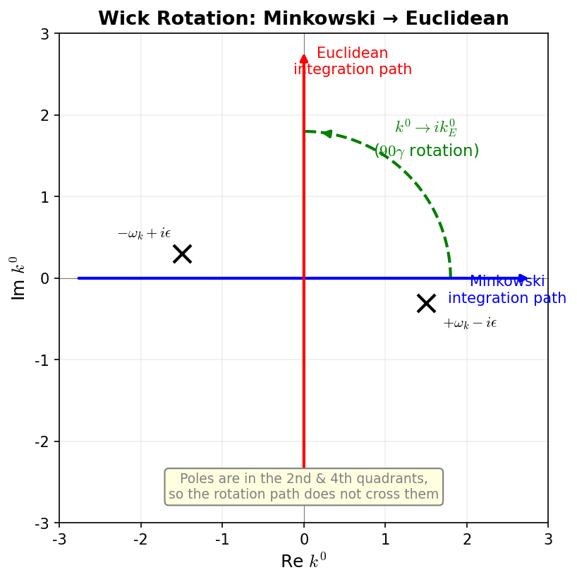
Fig. D.1: The complex \(\ell_0\) plane for Wick rotation. The Minkowski integration contour (blue, real axis) is rotated counterclockwise by \(90°\) to the Euclidean integration contour (red, imaginary axis). Due to the \(i\varepsilon\) prescription, the poles (× marks) are in the 2nd quadrant (negative real part, positive imaginary part) and 4th quadrant (positive real part, negative imaginary part), so no poles are crossed during the rotation through the 1st and 3rd quadrants, preserving the integral value.
What we use here is the "contour deformation principle" derived from Cauchy's theorem in complex analysis. Simply put, "if you continuously deform an integration contour in the complex plane without crossing any singularities (poles), the value of the integral doesn't change."
Let me give an intuitive explanation of why this holds. When a function \(f(z)\) in the complex plane behaves smoothly in a region without explosions like \(1/z\) (i.e., no poles) — in regions without poles, you can freely deform the integration contour without changing the integral value. This is called Cauchy's theorem (I'll leave the rigorous proof to complex analysis textbooks, but here we'll just use the fact that "contour deformation is free in regions without poles").
🔵 Kai: Would it be easier to imagine with an analogy, like water flow or something?
🟡 Lina: Good idea. Let me use a water flow analogy (this is just a metaphor, not an exact correspondence, but it's useful for building intuition). Imagine a flat water tank with several holes where water gushes out (= poles). Consider stretching a string from point A to point B in the tank and measuring the water flow crossing the string. If you change the path of the string, as long as there are no gushing holes between the paths, the flow rate doesn't change, right? But if there's a hole between the paths, the flow rate changes by the amount of water gushing from that hole. Something similar happens in complex integration — as long as you don't encircle poles, the integral value doesn't change no matter how you deform the contour.
⚪ Mei: As long as you move the string avoiding the holes = poles, the flow rate = integral value stays constant. A clear metaphor.
🟡 Lina: To be a bit more specific, when you connect the original contour (real axis) and the new contour (imaginary axis) at their endpoints to form a closed contour, if there are no poles inside it, the integral along the closed contour is zero (Cauchy's integral theorem). "Connecting at the endpoints" means joining the ends of the real axis (\(\pm R\)) to the ends of the imaginary axis (\(\pm iR\)) with quarter-circle arcs. As \(R \to \infty\), if the integrand decays sufficiently fast, the integral along the arcs vanishes, so closed contour integral = real axis integral + imaginary axis integral (reversed direction) = 0. This means the real axis integral equals the imaginary axis integral. In our case, since the denominator grows as a high power of \(\ell_0\), the integrand approaches zero rapidly as \(1/|\ell_0|^{2n}\) for \(|\ell_0| \to \infty\) — so the arc contributions indeed vanish. I'll leave the rigorous proof to complex analysis textbooks, but here we'll use the fact that "we can rotate the contour while avoiding poles."
Specifically:
where \(\ell_0^E\) is real. Then:
where \(\ell_E^2 = (\ell_0^E)^2 + \vec{\ell}^{\,2}\) is the squared norm in 4-dimensional Euclidean space.
⚪ Mei: What happens to the integration measure?
🟡 Lina: Since \(d\ell_0 = i\,d\ell_0^E\):
Application to the Standard Form
🟡 Lina: Let's apply the Wick rotation to equation (D.28):
The denominator is \((-\ell_E^2 - \Delta)^2 = [-(\ell_E^2 + \Delta)]^2 = (-1)^2(\ell_E^2 + \Delta)^2 = (\ell_E^2 + \Delta)^2\), so:
🔵 Kai: \((-1)^2 = 1\) made the sign in the denominator disappear! And since \(\ell_E^2 + \Delta\) is always positive, we can integrate with confidence.
🟡 Lina: Exactly. In Euclidean space the integral is spherically symmetric, so we can use 4-dimensional spherical coordinates.
Integration in 4-Dimensional Spherical Coordinates
🟡 Lina: The integral of a spherically symmetric integrand \(f(\ell_E^2)\) in 4-dimensional Euclidean space can be understood by analogy with 3 dimensions. In 3 dimensions we can write \(\int d^3x\,f(r^2) = 4\pi\int_0^\infty r^2\,dr\,f(r^2)\), right? You multiply by the surface area \(4\pi r^2\) and integrate radially. In 4 dimensions it's the same: we integrate with "surface area of a 4-dimensional sphere" \(\times\) \(\ell_E^3\,d\ell_E\):
Here \(2\pi^2\) is the surface area of the 4-dimensional unit sphere (I'll derive this shortly). \(\ell_E^3\) is the radial part of the volume element; in \(d\) dimensions it's generally \(\ell_E^{d-1}\). The reason is that just as \(d^3x = r^2\sin\theta\,dr\,d\theta\,d\phi\) in 3 dimensions, in \(d\) dimensions the volume element also decomposes into "radial direction \(d\ell_E\)" \(\times\) "angular surface element." Integrating out all the angles gives the surface area of a \((d-1)\)-dimensional sphere of radius \(\ell_E\): \(S_d \cdot \ell_E^{d-1}\). So the volume element becomes \(S_d \cdot \ell_E^{d-1}\,d\ell_E\). In 4 dimensions that's the \(\ell_E^3\,d\ell_E\) part.
🔵 Kai: In 3 dimensions it's \(r^2\,dr\), in 4 dimensions \(\ell_E^3\,d\ell_E\) — so the power goes up by one each time the dimension increases by one.
🟡 Lina: Exactly. In general, in \(d\) dimensions:
⚪ Mei: I'd like to check the 3-dimensional case. Substituting \(d = 3\) gives \(S_3 = 2\pi^{3/2}/\Gamma(3/2)\), but what's \(\Gamma(3/2)\)?
🟡 Lina: Just use the recursion relation from before. \(\Gamma(3/2) = \frac{1}{2}\Gamma(1/2) = \sqrt{\pi}/2\). So \(S_3 = 2\pi^{3/2}/(\sqrt{\pi}/2) = 4\pi\). The familiar surface area of a sphere.
⚪ Mei: I see, \(4\pi\) indeed comes out. The formula is confirmed to be consistent.
🔵 Kai: The surface area of a 4-dimensional sphere being \(2\pi^2\) is strange. 3 dimensions gives \(4\pi\) and 4 dimensions gives \(2\pi^2\)...
🟡 Lina: Here \(S_d\) represents "the surface area of the unit sphere in \(d\)-dimensional space" — that is, the area of a \((d-1)\)-dimensional sphere. \(S_d = 2\pi^{d/2}/\Gamma(d/2)\) can be derived from the \(d\)-dimensional version of the Gaussian integral. Substituting \(d = 4\) gives \(S_4 = 2\pi^2/\Gamma(2) = 2\pi^2\), matching the coefficient in equation (D.32). In other words, equation (D.32) is the special case \(d = 4\) of equation (D.33).
The key idea is that rewriting the \(d\)-dimensional Gaussian integral \(\int d^d x\,e^{-|\vec{x}|^2} = \pi^{d/2}\) in spherical coordinates gives \(S_d \int_0^\infty r^{d-1}e^{-r^2}dr\).
🔵 Kai: Wait a moment. Why is \(\int d^d x\,e^{-|\vec{x}|^2} = \pi^{d/2}\)?
🟡 Lina: Good question. Since \(|\vec{x}|^2 = x_1^2 + x_2^2 + \cdots + x_d^2\), we can factor \(e^{-|\vec{x}|^2} = e^{-x_1^2}\cdot e^{-x_2^2}\cdots e^{-x_d^2}\) into a product of exponentials for each axis. The integral also factorizes as \(\int d^d x = \int dx_1 \int dx_2 \cdots \int dx_d\), so the whole thing becomes a product of \(d\) independent 1-dimensional Gaussian integrals \(\int_{-\infty}^{\infty} e^{-x_i^2}dx_i = \sqrt{\pi}\) (this \(\sqrt{\pi}\) value corresponds to setting \(a = 2\) in equation (C.1) of Appendix C). So \(\sqrt{\pi}^{\,d} = \pi^{d/2}\). Setting \(a = 2\) in equation (C.1) of Appendix C gives \(\int e^{-q^2}dq = \sqrt{\pi}\), and this is raised to the \(d\)th power.
⚪ Mei: Since each axis is independent, the \(d\)-dimensional Gaussian integral is the \(d\)th power of the 1-dimensional one. Beautiful.
🔵 Kai: Ah, because the argument of the exponential is a sum of squares of each variable, it can be decomposed into a product. The radial integral \(\int_0^\infty r^{d-1}e^{-r^2}dr\) — as it stands, it doesn't look like a gamma function to me...
🟡 Lina: Good observation. Substitute \(t = r^2\). Then \(r = \sqrt{t}\) so \(dr = dt/(2\sqrt{t})\), \(r^{d-1} = t^{(d-1)/2}\). Multiplying gives \(r^{d-1}dr = t^{(d-1)/2} \cdot dt/(2\sqrt{t}) = \frac{1}{2}t^{d/2-1}dt\). So \(\int_0^\infty r^{d-1}e^{-r^2}dr = \frac{1}{2}\int_0^\infty t^{d/2-1}e^{-t}dt = \Gamma(d/2)/2\), which is exactly the definition of the gamma function.
Now we can equate the two results:
Solving for \(S_d\) gives \(S_d = 2\pi^{d/2}/\Gamma(d/2)\). For \(d = 4\), \(S_4 = 2\pi^2/\Gamma(2) = 2\pi^2\). That completes the derivation.
⚪ Mei: So a single formula \(S_d = 2\pi^{d/2}/\Gamma(d/2)\) for the \(d\)-dimensional surface area unifies both \(4\pi\) for \(d = 3\) and \(2\pi^2\) for \(d = 4\). And when using dimensional regularization with non-integer \(d\), as Lina mentioned, this formula can be used as-is.
Basic Momentum Integral Formulas
🟡 Lina: With the Wick rotation and spherical coordinates, we can evaluate the standard integrals that appear in loop calculations. Let me summarize the results.
Basic Integral in Euclidean Space
🟡 Lina: With \(\Delta > 0\), the basic integral in 4-dimensional Euclidean space:
🔵 Kai: How do you derive this?
🟡 Lina: Using equation (D.32):
Substituting \(u = \ell_E^2\), we get \(du = 2\ell_E\,d\ell_E\), \(\ell_E^3\,d\ell_E = \frac{1}{2}u\,du\), so:
(Let me organize the prefactor. \(\frac{2\pi^2}{(2\pi)^4} = \frac{2\pi^2}{16\pi^4} = \frac{2}{16\pi^2} = \frac{1}{8\pi^2}\). Multiplying by the \(\frac{1}{2}\) from the \(u\) substitution gives \(\frac{1}{8\pi^2} \times \frac{1}{2} = \frac{1}{16\pi^2} = \frac{1}{(4\pi)^2}\).)
🔵 Kai: I see, so the \(1/(4\pi)^2\) coefficient comes from here. That's a factor I often see in loop calculations.
🟡 Lina: Right, it's sometimes called the "loop factor \(1/(4\pi)^2\)." To bring this integral into beta function form, we look for a substitution that maps the range \([0,\infty)\) to \([0,1]\). Setting \(t = u/(u + \Delta)\) works: \(u = 0\) gives \(t = 0\), \(u \to \infty\) gives \(t \to 1\). We have \(u = \Delta t/(1-t)\), \(du = \Delta/(1-t)^2\,dt\), \(u + \Delta = \Delta/(1-t)\). Rewriting the integrand:
Multiplying by \(du = \Delta/(1-t)^2\,dt\):
When \(u: 0 \to \infty\), \(t: 0 \to 1\), so:
⚪ Mei: Ah, this is exactly the form \(B(2, n-2) = \int_0^1 t^{2-1}(1-t)^{(n-2)-1}dt\).
🟡 Lina: Exactly. This is the beta function \(B(a,b) = \int_0^1 t^{a-1}(1-t)^{b-1}dt = \frac{\Gamma(a)\Gamma(b)}{\Gamma(a+b)}\) introduced earlier. Here \(a = 2\), \(b = n-2\), so:
Substituting:
Since \(\Gamma(2) = 1! = 1\), this gives us equation (D.34).
⚪ Mei: For \(n = 2\), \(\Gamma(0)\) diverges. Does that mean the integral is infinite?
🟡 Lina: Sharp! Exactly so. When \(n = 2\), \(\Gamma(n-2) = \Gamma(0) = \infty\), and the integral diverges logarithmically. This is the identity of the "infinity appearing in loops" — the ultraviolet divergence — that we saw in Ch. 13. In dimensional regularization, this divergence is captured as a \(1/\epsilon\) pole by setting \(d = 4 - 2\epsilon\). See Ch. 14 for details.
✅ Comprehension Check: Why does a divergence occur in the basic Euclidean integral formula (D.34) when \(n = 2\)? Mathematically, what function's property causes this?
Answer
When \(n = 2\), the formula contains \(\Gamma(n-2) = \Gamma(0)\) which diverges. The gamma function has a pole at \(z = 0\), so \(\Gamma(0) = \infty\). Physically, this corresponds to the ultraviolet (logarithmic) divergence of the loop integral, which in dimensional regularization is captured as a \(1/\epsilon\) pole with \(d = 4 - 2\epsilon\).
📝 Exercises:
- Explicit calculation of equation (D.34) for \(n = 3\) and dimensional verification → Problem B-7. General Feynman Parameter Formula (\(n = 3\))
- Momentum integral in 2-dimensional Euclidean space and comparison with 4 dimensions → Problem M-1. Complete Reduction of a One-Loop Integral Using Feynman Parameters
The Case \(n = 2\) (Logarithmic Divergence)
🟡 Lina: The \(n = 2\) case is the most important, so let's also examine the divergence behavior using a different method. In equation (D.34), \(\Gamma(0) = \infty\) appeared and the formula couldn't be used directly. So instead, we cut off the upper limit of integration at a finite value \(\Lambda^2\) — meaning "we ignore contributions from momenta exceeding \(\Lambda\)." This \(\Lambda\) is called the ultraviolet cutoff. Physically, it corresponds to "the maximum energy scale where the theory is valid."
🔵 Kai: So you manually impose an upper energy limit saying "we only trust up to here."
🟡 Lina: That's right. We rewrite the numerator \(u\) as \((u+\Delta) - \Delta\) — this is just the identity of adding and subtracting \(\Delta\). This produces a form that can be canceled with \((u+\Delta)\) in the denominator:
Integrating each term: The first term gives \(\int_0^{\Lambda^2} \frac{du}{u+\Delta} = [\ln(u+\Delta)]_0^{\Lambda^2} = \ln(\Lambda^2+\Delta) - \ln\Delta = \ln\frac{\Lambda^2+\Delta}{\Delta}\). The second term gives \(\int_0^{\Lambda^2} \frac{\Delta\,du}{(u+\Delta)^2} = \Delta\left[-\frac{1}{u+\Delta}\right]_0^{\Lambda^2} = \Delta\left(-\frac{1}{\Lambda^2+\Delta} + \frac{1}{\Delta}\right) = 1 - \frac{\Delta}{\Lambda^2+\Delta} = \frac{\Lambda^2}{\Lambda^2+\Delta}\). Combining:
When \(\Lambda \gg \sqrt{\Delta}\):
🔵 Kai: Ah, \(\ln\Lambda^2\) appeared. It diverges logarithmically as the cutoff increases.
🟡 Lina: Be careful — as we saw in the derivation of equation (D.34), the complete loop integral has a factor of \(\frac{1}{(4\pi)^2}\) multiplied in front. So the result of equation (D.28) with \(n = 2\) after Wick rotation is \(\frac{i}{(4\pi)^2}\left(\ln\frac{\Lambda^2}{\Delta} - 1 + \cdots\right)\).
🔵 Kai: So it diverges logarithmically with the cutoff \(\Lambda\). That's milder than a power-law divergence like \(\Lambda^2\), but it's still infinite...
🟡 Lina: True. But this logarithmic divergence can be handled by renormalization. As we learned in Ch. 14.
Numerator with Loop Momentum
🟡 Lina: Formulas for when the numerator contains loop momentum \(\ell_E^\mu\) or \(\ell_E^\mu \ell_E^\nu\) are also important:
Odd powers:
This is obvious from symmetry.
Even powers:
🔵 Kai: Why does \(\delta^{\mu\nu}/4\) appear?
🟡 Lina: In Euclidean space the integral is symmetric under 4-dimensional rotations, so the result must be a rotation-invariant tensor. The only rank-2 symmetric tensor that's rotation-invariant is \(\delta^{\mu\nu}\). So we can write \(\int \ell_E^\mu \ell_E^\nu (\cdots) = C\,\delta^{\mu\nu}\). To determine the coefficient \(C\), contract both sides by setting \(\mu = \nu\) and summing. The left side becomes \(\int \ell_E^2 (\cdots)\), and the right side becomes \(C \cdot \delta^{\mu\mu} = 4C\) (since \(\delta^{\mu\mu} = 4\) in 4 dimensions). Comparing gives \(C = \frac{1}{4}\int \ell_E^2 (\cdots)\).
⚪ Mei: So the "4" is the number of dimensions. Divide by 4 because it's 4 dimensions. In a 3-dimensional integral, it would be \(\delta^{\mu\nu}/3\).
🟡 Lina: Exactly. In general, the same argument in \(d\) dimensions gives \(\delta^{\mu\nu}/d\). This is a fact used in dimensional regularization with \(d = 4 - 2\epsilon\). Now let's compute the right-hand side of equation (D.38). Writing \(\ell_E^2\) in the numerator as \((\ell_E^2 + \Delta) - \Delta\):
Applying equation (D.34):
🔵 Kai: Even with \(\ell_E^2\) in the numerator, just adding and subtracting \(\Delta\) reduces it to the basic formula. The same technique as the cutoff calculation for \(n = 2\) earlier.
⚪ Mei: Using the recursion relation \(\Gamma(z+1) = z\,\Gamma(z)\) that Lina taught us repeatedly: \(\Gamma(n-1) = (n-2)\Gamma(n-2) = (n-2)(n-3)\Gamma(n-3)\) so \(\frac{\Gamma(n-3)}{\Gamma(n-1)} = \frac{1}{(n-2)(n-3)}\). Similarly \(\Gamma(n) = (n-1)(n-2)\Gamma(n-2)\) so \(\frac{\Gamma(n-2)}{\Gamma(n)} = \frac{1}{(n-1)(n-2)}\).
🟡 Lina: Good. Taking the difference (finding a common denominator):
🔵 Kai: Using the recursion relation three times gives \(\Gamma(n) = (n-1)(n-2)(n-3)\Gamma(n-3)\), so the denominator is exactly \(\Gamma(n)/\Gamma(n-3)\).
🟡 Lina: Exactly. \(\frac{2}{(n-1)(n-2)(n-3)} = \frac{2\,\Gamma(n-3)}{\Gamma(n)}\). Combining with the \(\delta^{\mu\nu}/4\) out front gives \(\frac{\delta^{\mu\nu}}{4} \times \frac{2\,\Gamma(n-3)}{\Gamma(n)} = \frac{\delta^{\mu\nu}}{2}\cdot\frac{\Gamma(n-3)}{\Gamma(n)}\), so:
Result Translated Back to Minkowski Space
🟡 Lina: In actual calculations, we often want the result in Minkowski space before the Wick rotation. Including the \(i\) factor from equation (D.31):
🔵 Kai: Where does the \((-1)^n\) come from?
🟡 Lina: When transferring the Minkowski integral to Euclidean space, two effects combine:
- From \(d^4\ell = i\,d^4\ell_E\) (equation (D.30)), one factor of \(i\) comes out
- \(\ell^2 - \Delta \to -\ell_E^2 - \Delta = -(\ell_E^2 + \Delta)\)
⚪ Mei: So the integration measure produces \(i\), and the denominator produces \((-1)^n\).
🟡 Lina: Exactly. The \(n\)th power of the denominator transforms as \((\ell^2 - \Delta + i\varepsilon)^n = [-(\ell_E^2 + \Delta - i\varepsilon)]^n = (-1)^n(\ell_E^2 + \Delta - i\varepsilon)^n\). In Euclidean space \(\ell_E^2 + \Delta > 0\), so there's no worry about the denominator vanishing, and \(\varepsilon\) is no longer needed — we can safely take \(\varepsilon \to 0^+\):
Since \(n\) is a positive integer, \((-1)^n = \pm 1\). The reciprocal of \(\pm 1\) is itself, so \(1/(-1)^n = (-1)^n\) (check: \((-1)^n \times (-1)^n = (-1)^{2n} = 1\)). Therefore \(\frac{i}{(-1)^n} = i \cdot (-1)^n\), and the overall coefficient is \(i\,(-1)^n\). Equation (D.31) was the \(n = 2\) case where \((-1)^2 = 1\), so only \(i\) remained, but for general \(n\) this \((-1)^n\) persists.
⚪ Mei: Let me verify: for \(n = 2\), \((-1)^2 = 1\) so the coefficient is \(i/(4\pi)^2 \cdot \Gamma(0)/\Gamma(2) \cdot 1/\Delta^0\), but since \(\Gamma(0)\) diverges, this formula can't be used as-is — that's the ultraviolet divergence. For \(n = 3\), \((-1)^3 = -1\) gives \(-i/(4\pi)^2 \cdot \Gamma(1)/\Gamma(3) \cdot 1/\Delta = -i/(32\pi^2\Delta)\). This one is finite.
🟡 Lina: Correct. That confirms equation (D.40).
Comprehension check: State the two essential effects of the Wick rotation
- It changes the Minkowski metric \(\ell^2 = \ell_0^2 - \vec{\ell}^{\,2}\) to the Euclidean metric \(-\ell_E^2 = -(\ell_0^E)^2 - \vec{\ell}^{\,2}\), avoiding poles in the integrand.
- The integral becomes spherically symmetric in 4 dimensions, making the angular integration tractable.
Summary: Toolkit at a Glance
🟡 Lina: Finally, let me list the main formulas of this Appendix in one place. Come back here whenever you get lost in loop calculations.
Table D.3: Summary of main formulas in Appendix D
| Number | Formula | Use |
|---|---|---|
| (D.3)–(D.4) | \([\phi] = 1\), \([\psi] = 3/2\) | Determining dimensions of fields and coupling constants |
| (D.7) | \(\eta^{\mu\nu} = (+,-,-,-)\) | Metric convention |
| (D.21)–(D.22) | Fourier transform convention | Tracking \(2\pi\) factors |
| (D.24) | Feynman parameter (2 factors) | Combining denominators |
| (D.25) | Feynman parameter (\(n\) factors) | Combining multiple propagators |
| (D.26) | Unequal powers | Combining denominators with different powers |
| (D.29)–(D.30) | \(\ell_0 \to i\ell_0^E\), \(d^4\ell = i\,d^4\ell_E\) | Wick rotation |
| (D.34) | Basic integral in Euclidean space | Scalar-type loop integrals |
| (D.37)–(D.39) | Numerator with \(\ell\) | Tensor-type loop integrals |
| (D.40) | Final result in Minkowski space | Computing physical amplitudes |
🔵 Kai: With all this, it seems like we can concretely carry out the renormalization calculations in Chapters 13–14. But one thing I'm curious about: for two loops or more, won't there be many Feynman parameters, making the final \(x\) integral incredibly complicated?
🟡 Lina: Good question. Indeed, at two loops and beyond, multiple integrals over Feynman parameters remain, and often they can't be performed analytically. In such cases, numerical integration or special functions (polylogarithms, etc.) are used. But the procedure up to performing the momentum integral — combine denominators, complete the square, Wick rotate, integrate in spherical coordinates — is the same.
🔵 Kai: I see that the procedure itself is the same, with only the final Feynman parameter integral becoming harder. But at two loops, there are two loop momenta, right? Do you do the Wick rotation twice? Or rotate both time components simultaneously?
🟡 Lina: Yes, for each loop momentum \(k_1\), \(k_2\), you Wick rotate \(k_{1,0} \to ik_{1,0}^E\), \(k_{2,0} \to ik_{2,0}^E\). The typical approach is to integrate one loop momentum first (using the 1-loop formulas at this step), then apply the same procedure again for the remaining one.
🔵 Kai: So it has a nested structure. Fix the outer loop, deal with the inner one first — like nested loops in programming. But if the result of integrating the inner loop depends on the outer loop momentum, doesn't the outer integral become complicated again? Doesn't it eventually become intractable somewhere?
🟡 Lina: Good concern. Indeed, the result of the inner loop integral remains as a function of the outer loop momentum and Feynman parameters, making the outer integral generally more complex than a 1-loop calculation. Often it can't be written in closed form. But the procedure itself — Feynman parameters → completing the square → Wick rotation → spherical coordinates — is the same, so in principle the calculation is feasible.
🔵 Kai: I see. So conversely, while the framework for calculation can in principle be set up for any loop order using just this appendix's tools, whether the answer can actually be written in closed form is a separate matter.
⚪ Mei: To organize: the skeleton of loop calculations is the 4 steps "①Combine denominators with Feynman parameters → ②Complete the square to standard form → ③Wick rotate to Euclidean space → ④Integrate in spherical coordinates." At two loops and beyond, these 4 steps are applied repeatedly for each loop momentum, with a multiple integral over Feynman parameters remaining at the end.
🔵 Kai: Got it, 4 steps memorized. But one more thing — this toolkit is for when "the integral converges," right? For divergent cases (\(n = 2\), etc.), you still need separate treatment with cutoffs or dimensional regularization. The toolkit alone isn't self-contained.
🟡 Lina: Exactly right. This appendix is the toolkit for "bringing the integral to standard form," while the treatment of divergences — regularization and renormalization — is the job of Ch. 14. But without these 4 steps, you couldn't even identify "what is diverging" in the first place. So it's an essential foundation.
🔵 Kai: Use the toolkit to identify "what diverges," then delegate the treatment to Chapter 14 — the division of responsibilities is clear and easy to understand.
References
- Quantum Field Theory and the Standard Model (M. Schwartz) Appendix B "Regularization"
- An Introduction to Quantum Field Theory (Peskin & Schroeder) Appendix A "Some Useful Formulas"
- Quantum Field Theory (Srednicki) Chapter 14 "Loop Integrals in Vacuum"
Feedback on this page
Let us know if something was unclear, incorrect, or could be improved.