Chapter 4: The Mathematics of Minkowski Spacetime — Metric, Four-Vectors, and Tensors¶
Story so far: In Ch. 3, we derived the spacetime interval \(ds^2 = -(cdt)^2 + dx^2 + dy^2 + dz^2\) from the principle of relativity and the invariance of the speed of light, and obtained the Lorentz transformation as the coordinate transformation that preserves \(ds^2\). From there, we drew the physical consequences of relativity of simultaneity, time dilation, and length contraction, completing the "physics" of special relativity. However, to proceed to general relativity, we need to rewrite this physics in mathematical expressions that do not depend on the coordinate system.
Goals of this chapter
- Reorganize the special relativity physics obtained in Ch. 3 using the mathematical language needed to proceed to general relativity
- Specifically, we will establish natural units (\(c = 1\)), index notation and Einstein's summation convention, the Minkowski metric \(\eta_{\mu\nu}\), four-vectors (contravariant and covariant), and the basics of tensors
- This will prepare us to handle "curved spacetime"
4.1 Minkowski Spacetime and the Metric Tensor¶
🟡 Lina: In the opening of Section 3 of Ch. 3, I said "we'll postpone rank-1 tensors (four-vectors) for later." Now that we've dealt with Lorentz transformations and their physical consequences, it's time to continue up the tensor hierarchy—rank-1 tensors (four-vectors) and rank-2 tensors (the metric \(\eta_{\mu\nu}\)). First, as preparation, let's introduce natural units and index notation. But before that, let's confirm the overall picture of Minkowski spacetime in Fig. 4.1 "The light cone in Minkowski spacetime".
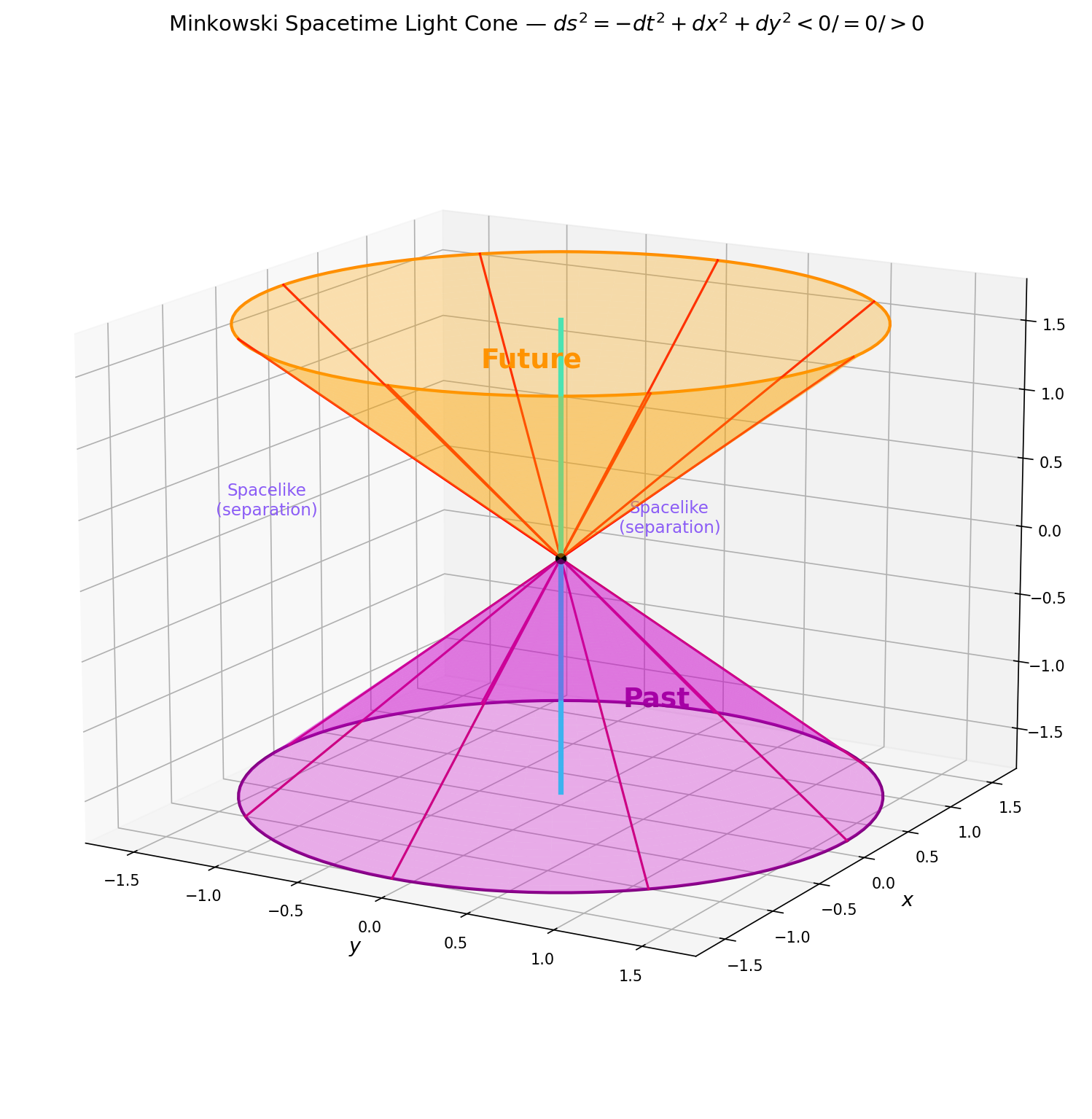
Fig. 4.1: The light cone in Minkowski spacetime. From any given event, the interior of the cone formed by light rays represents the future and past (causally connected), while the exterior is spacelike (causally disconnected). The sign of \(ds^2 = -(c\,dt)^2 + dx^2 + dy^2 + dz^2\) (in this chapter, with \(c = 1\): \(ds^2 = -dt^2 + dx^2 + dy^2 + dz^2\)) determines the region (\(< 0\): timelike, \(= 0\): lightlike, \(> 0\): spacelike). The blue line is the worldline of a massive particle (always confined within the light cone).
🔵 Kai: Looking at Fig. 4.1 "The light cone in Minkowski spacetime", the interior of the light cone is "causally connected" and the exterior is "causally disconnected"… meaning information can't travel faster than light, so you can't influence events outside your light cone.
🟡 Lina: Exactly. And the worldline of a massive particle (the blue line in the figure) always stays within the light cone—because nothing can exceed the speed of light. The sign of \(ds^2\) expresses this structure mathematically—\(ds^2 < 0\) means timelike (inside the light cone), \(ds^2 = 0\) means lightlike (on the surface of the light cone), and \(ds^2 > 0\) means spacelike (outside the light cone).
The \(c = 1\) Unit System (Natural Units)¶
🟡 Lina: From here on, we'll use units where \(c = 1\) to make the equations cleaner. This is a type of unit system called natural units, where setting the speed of light \(c\) to 1 allows us to treat time and space in the same units.
🔵 Kai: What does it mean to set the speed of light to 1?
🟡 Lina: We measure time in "meters." "1 meter of time" means the time it takes light to travel 1 meter—that is, \(1/c \approx 3.3\) nanoseconds. Then
Conversely, if we measure time in seconds and length in "light-seconds" (the distance light travels in 1 second \(\approx 3 \times 10^8\) m), we also get \(c = 1\). The point is measuring time and length in the same units.
⚪ Mei: How do the equations change specifically?
✅ Comprehension Check: What is the natural unit system (\(c = 1\))? And what are its advantages?
Answer
A unit system where the speed of light \(c\) is set to 1, allowing time and space to be treated in the same units. The equations become simpler by eliminating factors of \(c\), and the advantage is "not having to worry about where to place \(c\)." When you need to return to SI units, you can restore \(c\) through dimensional analysis.
🟡 Lina: Let me list a few examples.
Table 4.1: Comparison of physical formulas in SI units and natural units
| SI Units | Natural Units (\(c=1\)) |
|---|---|
| \(E = mc^2\) | \(E = m\) |
| \(\tau = t\sqrt{1 - v^2/c^2}\) | \(\tau = t\sqrt{1 - v^2}\) |
| \(\gamma = 1/\sqrt{1 - v^2/c^2}\) | \(\gamma = 1/\sqrt{1 - v^2}\) |
| \(ds^2 = -c^2 dt^2 + dx^2 + dy^2 + dz^2\) | \(ds^2 = -dt^2 + dx^2 + dy^2 + dz^2\) |
| \(v/c\) (dimensionless velocity) | \(v\) (velocity in units of the speed of light, \(0 \le v \le 1\)) |
🔵 Kai: Energy and mass become the same quantity?
🟡 Lina: Yes. The rest energy of a mass \(m\) kg is \(E = mc^2\) joules, but in natural units it's simply \(E = m\). Think of it as measuring both mass and energy in the same units (for example kg, or eV).
💡 Tip for getting used to it: Being told "measure mass in kg and energy in kg too" might be confusing at first. But if you adopt the view that "energy and mass are fundamentally the same thing (interchangeable via \(E=mc^2\))," it's a natural choice. In particle physics, both mass and energy are routinely measured in eV—for example, "the electron mass is 511 keV" (strictly \(511\ \mathrm{keV}/c^2\), but in natural units we drop the \(c\)). The biggest advantage in relativistic calculations is "not having to worry about units."
⚪ Mei: So when you want to convert back to SI units, you just restore \(c\) through dimensional analysis.
🟡 Lina: Exactly. For example, if \(E = m\), to match the dimensions of energy \([\text{kg}\cdot\text{m}^2/\text{s}^2]\) with mass \([\text{kg}]\), you multiply by \(c^2\) (dimensions \([\text{m}^2/\text{s}^2]\)) to get \(E = mc^2\). The natural unit system's advantage is "not having to worry about where to place \(c\)." Write equations simply with \(c = 1\), and if you need numerical values in SI at the end, restore \(c\) through dimensional analysis. This convention is standard in relativistic calculations.
Related unit systems
- Natural units: \(c = 1\). Used in relativity. Adopted in this chapter.
- Geometrized units: \(G = c = 1\). Newton's gravitational constant is also set to 1. Often used from Ch. 8 onward in general relativity.
- Planck units: \(G = c = \hbar = 1\). Used in quantum gravity (appears in Ch. 25).
- Particle physics natural units: \(\hbar = c = 1\). Used in quantum mechanics and quantum field theory.
This book will clearly state "the unit system for this chapter" at the beginning of each chapter, so be careful not to get confused.
🟡 Lina: In natural units, the Lorentz transformation becomes
which is quite clean. The spacetime interval is also
In the chapters that follow, we'll use natural units (\(c = 1\)) unless otherwise stated. We may sometimes switch to geometrized units (\(G = c = 1\)), so check "the unit system for this chapter" at the beginning of each chapter.
📝 Exercises:
- Converting to natural units and restoring \(c\) → Problem B-1. Conversion to Natural Units and Restoring \(c\), Problem B-2. Time and Length in Natural Units
Numbering the Coordinates¶
🟡 Lina: Now let me introduce the notation for handling all four coordinates together.
The superscript numbers are indices, not powers. We write all four coordinates collectively as \(x^\mu\) (\(\mu = 0, 1, 2, 3\)). Why superscripts? As we'll learn later, there are two types of indices—"upper" and "lower"—and they transform differently. The infinitesimal displacement of coordinates \(dx^\mu\) transforms under Lorentz transformations by multiplying by \(\Lambda\), and such quantities are called "contravariant vectors," written with upper indices by convention—so coordinates naturally take upper indices. The precise meaning of "contravariant vector" will be defined in Section 2, so for now just remember "coordinates are written with upper indices."
🔵 Kai: Isn't it confusing whether \(x^2\) means "\(x\) squared" or "the \(y\) coordinate"?
🟡 Lina: It can be confusing at first, but you'll learn to distinguish from context. Here's a tip—when used as an index, Greek letters like \(\mu, \nu, \alpha, \beta, \ldots\) accompany it, as in \(x^\mu\). When a number appears directly (like \(x^2\)), if the surrounding text is "listing coordinate components," it's an index; if it's "in the middle of a calculation," it's a power. In this book, when there's potential confusion with powers, we may write \((x)^2\) or \(x^2\) (non-italic) to distinguish.
Notation conventions: - Greek letter indices (\(\mu, \nu, \alpha, \beta, \ldots\)) run from \(0, 1, 2, 3\) and refer to all 4 spacetime components - Latin letter indices (\(i, j, k, \ldots\)) run from \(1, 2, 3\) and refer to only the 3 spatial components
Einstein's Summation Convention¶
🟡 Lina: Now that we've introduced index notation, let me present the most important notational convention for studying general relativity.
Einstein's summation convention: When the same index appears once as an upper index and once as a lower index within a single term, sum over that index from 0 to 3. The summation symbol \(\sum\) is omitted.
🔵 Kai: What does that mean concretely?
🟡 Lina: Let's start with the simplest example. Given a four-vector \(A^\mu = (A^0, A^1, A^2, A^3)\), substituting specific values for the index \(\mu\) gives each component. Now, if we multiply \(A^\mu\) (upper index) with another quantity \(B_\mu\) (lower index) and write \(A^\mu B_\mu\)? You noticed that the index on \(B_\mu\) is lower. The precise definition of \(B_\mu\) will be introduced in Section 3, but for now just think of it as "a different type of quantity with 4 components, also a set of 4 numbers \((B_0, B_1, B_2, B_3)\)"—for example, \(B_\mu = (5, 2, 0, 3)\), just 4 specific numbers lined up, and that's OK. Why we distinguish upper and lower will become clear later, so at this stage just remember the rule "when the same index appears once up and once down, sum over it." Actually expanding it, since \(\mu\) appears once up (in \(A^\mu\)) and once down (in \(B_\mu\)), we substitute \(\mu = 0, 1, 2, 3\) and add:
A sum of 4 terms. You can see that the sum is implied just from the position of the indices, without writing \(\sum\).
🔵 Kai: Oh, so it's just abbreviating \(\sum_{\mu=0}^{3}\).
🟡 Lina: Exactly. Let's look at another example. Writing the Lorentz transformation in index notation gives \(x^{\mu'} = \Lambda^{\mu'}{}_{\nu}\,x^\nu\). Here \(x^{\mu'}\) is the coordinate in the transformed inertial frame \(S'\), with a prime (\('\)) on the index to indicate it's "a quantity in the \(S'\) frame." \(x^\nu\) is the coordinate in the original frame \(S\). \(\Lambda^{\mu'}{}_{\nu}\) is the \((\mu', \nu)\) component of the transformation matrix—the upper \(\mu'\) represents "the component number in the target frame (\(S'\))," and the lower \(\nu\) represents "the component number in the source frame (\(S\))." Since \(\nu\) appears once up (in \(x^\nu\)) and once down (in \(\Lambda^{\mu'}{}_{\nu}\)), the summation convention tells us to sum:
⚪ Mei: In both examples, we sum over one index to get 4 terms—the same pattern.
🟡 Lina: Right. And this structure of "multiplying components one by one and adding" is the same form as the inner product you learned in high school. A single-index contraction is essentially the same operation as an inner product.
🔵 Kai: So it's like a generalization of the inner product.
🟡 Lina: Exactly. Now let's use a quantity with two indices—the metric tensor \(\eta_{\mu\nu}\)—to rewrite the spacetime interval.
✅ Comprehension Check: What is Einstein's summation convention?
Answer
When the same index appears once as an upper index and once as a lower index within a single term, sum over that index from 0 to 3. The summation symbol \(\sum\) is omitted.
Terminology note: An index that is summed over by the convention (appearing once up and once down with the same letter) is called a dummy index. The result is the same regardless of which letter is used for a dummy index. For example, \(A^\mu B_\mu = A^\nu B_\nu\). An index that is not summed over is called a free index.
The Minkowski Metric \(\eta_{\mu\nu}\)¶
🟡 Lina: Next, I want to rewrite the spacetime interval in index notation. The expression \(ds^2 = -dt^2 + dx^2 + dy^2 + dz^2\) contains the infinitesimal displacements of all 4 coordinates, but if we can write it in one shot as \(ds^2 = \eta_{\mu\nu}\,dx^\mu\,dx^\nu\), the same form works regardless of how many coordinates there are. What we need for this is the concept of a "metric." Let's first build some intuition.
🔵 Kai: What is a metric?
🟡 Lina: In one word, it's a "ruler"—a tool that tells us "how to measure the distance between two points" in a space (or spacetime). Let's look at three examples of increasing difficulty. First, let me summarize the overall picture in Fig. 4.2 "Three examples of metrics. Left: flat plane (metric is constant \(\mathrm{diag}(1,1)\)). Center: sphere (metric is a function of coordinate \(\theta\)".
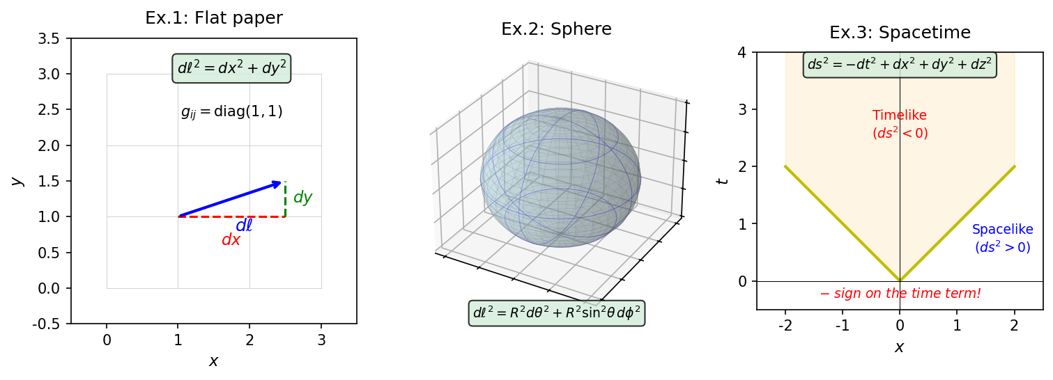
Fig. 4.2: Three examples of metrics. Left: flat plane (metric is constant \(\mathrm{diag}(1,1)\)). Center: sphere (metric is a function of coordinate \(\theta\) — the "scale markings on the ruler" change from place to place). Right: spacetime (the time term has a minus sign, giving a structure different from Euclidean geometry).
Example 1: On a Flat Sheet of Paper¶
On an ordinary plane, the distance between two points is determined by the Pythagorean theorem:
The information "coefficient 1 in front of \(dx^2\), coefficient 1 in front of \(dy^2\), no cross terms" is the metric of the plane. Written as a matrix:
The identity matrix—this is the metric of "flat space."
Example 2: The Surface of the Earth (A Curved Surface)¶
🟡 Lina: Next, consider the surface of the Earth (center of Fig. 4.2 "Three examples of metrics. Left: flat plane (metric is constant \(\mathrm{diag}(1,1)\)). Center: sphere (metric is a function of coordinate \(\theta\)"). To specify a position on the Earth, we use two angles. The first is the polar angle \(\theta\) (theta)—measured from the North Pole as \(\theta = 0\), increasing southward. The North Pole is \(\theta = 0\) (= 0°), the equator is \(\theta = \pi/2\) (= 90°), and the South Pole is \(\theta = \pi\) (= 180°). In geography, "latitude" is measured from the equator as 0° with north positive and south negative, but the physics polar angle starts at 0 at the North Pole and increases southward—note the opposite convention. The second is the longitude \(\phi\) (phi)—the east-west angle, ranging from \(0\) to \(2\pi\) (= 360°). Geographic longitude (\(-180°\) to \(+180°\)) has the same orientation but slightly different starting point and range. Using these two angles, the infinitesimal distance on the Earth's surface is
Intuitively, here's why—moving by \(d\theta\) in the latitudinal direction (north-south) means traveling along a great circle (a circle whose cross-section passes through the Earth's center) of radius \(R\), covering a distance \(R\,d\theta\). Moving by \(d\phi\) in the longitudinal direction (east-west) means traveling along a "small circle" (a line of latitude) whose radius at that latitude is \(R\sin\theta\), covering a distance \(R\sin\theta\,d\phi\). Why \(R\sin\theta\)? Because the distance from the Earth's rotation axis to the circle of latitude is \(R\sin\theta\)—at the North Pole (\(\theta = 0\)), \(\sin 0 = 0\) gives zero radius (a point), while at the equator (\(\theta = \pi/2\)), \(\sin(\pi/2) = 1\) gives radius \(R\) (maximum). And these two directions (north-south and east-west) are mutually perpendicular on the sphere—if you look at a globe, meridians and parallels always cross at right angles. On a small enough scale, a curved surface looks flat (just as the Earth's surface appears flat locally), so applying the Pythagorean theorem to the two perpendicular infinitesimal displacements gives
🔵 Kai: Wait a moment. Why is \(R\sin\theta\) the radius of the circle of latitude? The Earth's radius is \(R\), so why does \(\sin\theta\) appear?
🟡 Lina: Good question. Imagine a cross-section of the Earth. The horizontal distance from the rotation axis to the circle of latitude is \(R\sin\theta\) by trigonometry—at the North Pole (\(\theta = 0\)) you're on the axis so the distance is zero, at the equator (\(\theta = \pi/2\)) you're farthest from the axis at distance \(R\). So \(\sin\theta\) represents "how far you are from the rotation axis" as a fraction.
🔵 Kai: Ah, I see. So with \(\sin^2\theta\) in there, the "distance per degree of longitude" changes depending on location. Near the equator (\(\theta \approx \pi/2\)), \(\sin^2\theta \approx 1\) and it's large, but near the poles (\(\theta \approx 0\)), \(\sin^2\theta \approx 0\) and it's nearly zero.
🟡 Lina: Exactly. The "scale markings on the ruler" change from place to place—this is what it means for the metric to be a function of coordinates \(g_{ij}(\theta)\).
Unlike the identity matrix in Example 1, the diagonal components depend on position (\(\theta\)).
🔵 Kai: The metric of the plane is a constant matrix, and the metric of the sphere is a function of coordinates… so can you tell whether something is "flat" or "curved" by whether the metric depends on coordinates?
🟡 Lina: Good intuition, but it's not actually that simple. Even on a flat plane, if you use polar coordinates \((r, \theta)\), the metric becomes \(d\ell^2 = dr^2 + r^2 d\theta^2\), which is a function of coordinates. "Metric depends on coordinates" doesn't necessarily mean "curved." To truly determine whether something is curved, you need a more refined tool (the curvature tensor, appearing in Ch. 12). But at this stage, the intuition "non-constant metric → possibly curved" is sufficient.
Example 3: Spacetime¶
🟡 Lina: And now spacetime (right side of Fig. 4.2 "Three examples of metrics. Left: flat plane (metric is constant \(\mathrm{diag}(1,1)\)). Center: sphere (metric is a function of coordinate \(\theta\)"). The spacetime interval derived in Section 2 of Ch. 3,
can also be written using a metric. For space alone, all signs would be positive, but the time term has a minus sign. This is the core of "spacetime has a geometry different from ordinary space," and it's the conclusion we derived from the invariance of the speed of light in Section 2.3 of Ch. 3.
🔵 Kai: So the metric doesn't just determine "how to measure distance"—it represents the very nature of the space itself.
🟡 Lina: Precisely. And in general relativity, this metric becomes position-dependent \(g_{\mu\nu}(x)\)—the same structure as how \(\sin^2\theta\) varied with position on the Earth's surface. The role that Newton's gravitational potential \(\Phi\) played is taken over by the metric tensor \(g_{\mu\nu}\) in general relativity. The metric is simultaneously a "ruler" and "the gravitational field itself"—this is the core idea of general relativity. But that's a story for later. First, let's write the flat spacetime metric in index notation.
⚪ Mei: The three examples increased in difficulty step by step—a constant metric, a coordinate-dependent metric, and a metric with mixed signs.
🟡 Lina: Right. And in special relativity, we deal with the third case—signs are mixed but the metric is constant. Let's use the summation convention to rewrite the spacetime interval in index notation. \(ds^2 = -dt^2 + dx^2 + dy^2 + dz^2\) can be written as
Here \(\eta_{\mu\nu}\) (eta) is called the Minkowski metric, and arranging its components as a \(4 \times 4\) matrix gives
🔵 Kai: In \(\eta_{\mu\nu}\,dx^\mu\,dx^\nu\), both \(\mu\) and \(\nu\) run from 0 to 3, so… that's a sum of 16 terms in total, right?
🟡 Lina: Yes. Look closely at the expression \(\eta_{\mu\nu}\,dx^\mu\,dx^\nu\)—you can see the letter \(\mu\) appears twice. The first time in \(\eta_{\mu\nu}\) as a lower index, and the second time in \(dx^\mu\) as an upper index. Since it appears once up and once down, the summation convention tells us to sum over \(\mu = 0, 1, 2, 3\). Similarly for \(\nu\)—it appears as a lower index in \(\eta_{\mu\nu}\) and as an upper index in \(dx^\nu\)—so we sum over that too. The result is a double sum over \(\mu\) and \(\nu\) giving \(4 \times 4 = 16\) terms. But \(\eta_{\mu\nu}\) is a diagonal matrix—meaning components where the row and column numbers differ (\(\mu \neq \nu\)) are all zero. For example, \(\eta_{01} = 0\), \(\eta_{12} = 0\), etc. So of the 16 terms, the 12 with \(\mu \neq \nu\) vanish, leaving only the 4 terms with \(\mu = \nu\):
🔵 Kai: Wow, 12 terms vanish at once leaving only 4! Diagonal matrices make things simple.
⚪ Mei: So the single expression \(\eta_{\mu\nu}\,dx^\mu\,dx^\nu\) determines "which sign goes with the square of which component"—once you specify the metric, the spacetime interval formula comes out automatically.
🟡 Lina: Exactly. This \(\eta_{\mu\nu}\) is the "ruler" of Minkowski spacetime—the metric tensor. In general relativity, this gets replaced by a position-dependent \(g_{\mu\nu}(x)\). That is the mathematical expression of "spacetime being curved."
📝 Exercises:
- Minkowski inner product, summation convention, and index notation → Problem B-3. Calculating the Minkowski Inner Product, Problem B-4. Components of a Covariant Vector, Problem B-5. Expansion of the Spacetime Interval into 16 Terms, Problem B-6. Relabeling Dummy Indices
Notation conventions in this book
Many symbols have appeared so far, so let me organize them. You can tell whether something is a four-vector, a matrix (tensor), 3-dimensional or 4-dimensional by the type of letter used.
| Type | Symbol | Examples |
|---|---|---|
| Four-vectors (Greek indices \(\mu,\nu,\ldots\)) | Uppercase Latin | \(A^\mu\), \(B_\mu\), \(V^\mu\), \(U^\mu\) (four-velocity) |
| Rank-2 tensors (metric) | Lowercase Greek | \(\eta_{\mu\nu}\), \(g_{\mu\nu}\) |
| Rank-2 and higher tensors (others) | Uppercase Latin | \(T^{\mu\nu}\), \(R_{\mu\nu\rho\sigma}\) |
| Transformation matrices | Uppercase Greek | \(\Lambda^{\mu'}{}_{\nu}\) (Lorentz transformation) |
| Coordinates/displacements | Traditional lowercase | \(x^\mu\), \(dx^\mu\) |
| 3-dimensional vectors | Lowercase + arrow | \(\vec{v}\), \(\vec{r}\), \(\vec{p}\), \(\vec{F}\) |
| 3-dimensional vector components (Latin indices \(i,j = 1,2,3\)) | Lowercase | \(v^i\), \(v^x\), \(v^y\), \(v^z\) |
Roughly: "Four-vectors are uppercase, metric is lowercase Greek, 3D uses arrows." However, there is one exception—the four-momentum \(p^\mu\) uses lowercase by historical convention. Since this is universal in physics textbooks, we adopt it as is.
4.2 Four-Vectors¶
Why Four-Vectors Are Needed¶
🟡 Lina: In Newtonian mechanics, position \((x, y, z)\) and velocity \((v_x, v_y, v_z)\) were 3-component vectors. But in special relativity, time and space mix together. So we need to represent physical quantities as 4-component vectors that include a time component—four-vectors.
🔵 Kai: What do they look like specifically?
The Displacement Four-Vector¶
🟡 Lina: The most fundamental four-vector is the infinitesimal displacement between two events:
Writing how this transforms under Lorentz transformations in index notation (component form):
🔵 Kai: Is this different from a matrix equation?
🟡 Lina: Yes. This is not the matrix itself, but an expression for one particular component. \(\mu'\) abstractly represents a component number (one of 0, 1, 2, 3)—substituting \(\mu' = 0\) gives the equation for \(dt'\), substituting \(\mu' = 1\) gives the equation for \(dx'\). A single equation summarizes all 4 components.
🟡 Lina: Here \(\Lambda\) (Lambda) is the Lorentz transformation matrix, and \(\Lambda^{\mu'}{}_{\nu}\) is its \((\mu', \nu)\) component. For a boost in the \(x\) direction with velocity \(v\):
🟡 Lina: For example, try computing the \(\mu' = 0\) component. By the summation convention, we sum over \(\nu\)—
🔵 Kai: Let me see, substituting \(\nu = 0, 1, 2, 3\) and adding… \(\Lambda^{0'}{}_{0}\,dx^0 + \Lambda^{0'}{}_{1}\,dx^1 + \Lambda^{0'}{}_{2}\,dx^2 + \Lambda^{0'}{}_{3}\,dx^3\). Plugging in the matrix components gives \(\gamma\,dt - \gamma v\,dx\)?
⚪ Mei: So \(dt' = \gamma(dt - v\,dx)\)—that matches the Lorentz transformation from before.
Definition of a Four-Vector¶
🟡 Lina: We just saw that \(dx^\mu\) gets mixed up under Lorentz transformations as \(dx^{\mu'} = \Lambda^{\mu'}{}_{\nu}\,dx^\nu\). It turns out that among the quantities appearing in physics, there are many others that mix in exactly the same way as \(dx^\mu\)—velocity, momentum, current density…. So it's convenient to give a name to quantities that share this "mixing rule."
🔵 Kai: What does "mix in the same way" mean specifically?
🟡 Lina: Given a set of 4 quantities \(V^\mu = (V^0, V^1, V^2, V^3)\), when we switch inertial frames from \(S\) to \(S'\), using the transformation matrix \(\Lambda\) (Lambda):
—that is, they transform with the same matrix \(\Lambda\) as \(dx^\mu\). Quantities with this property are called contravariant vectors. The \(dx^\mu\) itself is the first example of a contravariant vector.
🔵 Kai: Can you break this equation down a bit more?
🟡 Lina: Sure. Let's unpack \(V^{\mu'} = \Lambda^{\mu'}{}_{\nu}\,V^\nu\). Since \(\nu\) appears up (in \(V^\nu\)) and down (in \(\Lambda^{\mu'}{}_{\nu}\)), by the summation convention from Section 1.3, we sum over it. So this equation is shorthand for
A sum of 4 terms. Substituting specific values (0, 1, 2, 3) for \(\mu'\) gives each component in the \(S'\) frame.
🔵 Kai: That's the same structure as when Mei computed \(dx^{0'} = \gamma\,dt - \gamma v\,dx\) earlier.
🟡 Lina: Exactly. Intuitively, this equation says "take the \(S\) frame components \(V^0, V^1, V^2, V^3\), mix them together according to the conversion rule \(\Lambda\), and produce the \(S'\) frame component \(V^{\mu'}\)." It's the same structure as when you rotate a 3-dimensional vector and \((v_x, v_y, v_z)\) get mixed by the rotation matrix. The numerical values of the components change, but the vector itself (its physical content) doesn't change.
🔵 Kai: So, if the components \(V^{\mu'}\) computed by applying \(\Lambda\) match the values actually measured in the \(S'\) frame, then it's a contravariant vector?
🟡 Lina: Exactly right. You can always perform the calculation of multiplying by \(\Lambda\) on any set of 4 numbers. But the result won't necessarily match the correct values in the \(S'\) frame. In fact, some quantities have their components change in the "same direction" as the coordinate transformation, while others change in the "opposite direction"—this is the distinction between "covariant vectors" and "contravariant vectors," which we'll cover in detail in Section 3. For now, just remember that "upper indices (contravariant) and lower indices (covariant) transform in opposite ways."
🔵 Kai: So "whether applying \(\Lambda\) gives the correct answer" is the criterion for whether something is a contravariant vector.
🟡 Lina: Yes. Quantities that transform with the inverse matrix of \(\Lambda\) (lower index \(V_\mu\)) are called covariant vectors. The names come from co = "together with," contra = "against." Together with or against what? Against the change in coordinate scale markings. Under a transformation that makes the markings larger, if the components also get larger, that's covariant (co = changing together); if the components get smaller, that's contravariant (contra = changing in opposition). The following concrete example will help build your intuition. The representative example of a covariant vector is the gradient—the partial derivatives \(\partial\Phi/\partial x^\mu\) of some scalar field (for example, a quantity like the gravitational potential \(\Phi\) that has a definite value at each point of spacetime) form a covariant vector. We'll formally derive this in later chapters, but for now just remember "displacement \(dx^\mu\) is the representative of contravariant, gradient is the representative of covariant." Intuitively—consider a transformation that stretches the coordinate scale markings by a factor of 2.
Let me give a concrete example. Picture a number line. In 1 dimension, suppose a rod has length \(\Delta x = 3\) scale markings in the original coordinates. Now stretch the spacing of the markings by a factor of 2—meaning 1 new marking corresponds to 2 original markings of physical length. The physical positions haven't changed, but since the markings got bigger, reading the same position in the new coordinates gives half the numerical value—in coordinates, \(x' = x/2\). Then measuring the same rod gives \(\Delta x' = 3/2 = 1.5\) markings—the numerical value of the displacement became half because the markings got bigger. The basis (unit vector of the markings) got "bigger" in this transformation, yet the displacement component got "smaller." This is the meaning of "contravariant = changes in the opposite direction to the basis transformation."
🔵 Kai: Ah, when the ruler stretches, the numbers shrink. Opposite to the markings, so "contravariant."
On the other hand, consider the slope of a hill (gradient). In the original coordinates, "advancing 1 marking raises the height by 4 m." If we stretch the markings by a factor of 2, then 1 new marking corresponds to 2 original markings of distance. So in the new coordinates, "advancing 1 marking" actually means traveling 2 original markings, so the height rises by \(4 \times 2 = 8\) m—the numerical value of the gradient doubles. Under a transformation that makes coordinates "larger," the gradient also gets "larger." This is the meaning of "covariant = changes in the same direction as the coordinate transformation."
To summarize—under the same "stretch markings by factor 2" transformation, displacement components become half (opposite direction = contravariant), gradient components double (same direction = covariant). The matrices describing the transformation are different (\(\Lambda\) vs. \(\Lambda^{-1}\))—that's the essential distinction.
🔵 Kai: That example was 1-dimensional, but does the same idea hold in 4-dimensional spacetime?
🟡 Lina: Yes. In 4 dimensions the essence is the same—relative to how the coordinate markings change (\(\Lambda\)), components that change in the opposite direction are contravariant, and those that change in the same direction are covariant. The specific transformation formulas and usage will be covered in detail in Section 3; for now just remember "upper and lower transform in opposite ways." Contravariant vectors and covariant vectors together are collectively called four-vectors.
%%{init: {"theme": "default", "themeCSS": ".edgePath .path, .flowchart-link { stroke-width: 2px !important; }"}}%%
flowchart TB
    all["<b>A set of 4 numbers</b><br/>e.g., (t, x, m, 0) or anything"]
    all -->|"Transforms via Λ or Λ⁻¹"| four["<b>Four-vector</b>"]
    all -->|"Has no transformation law"| not4["Not a four-vector<br/>e.g., (t, x, m, 0)"]
    four --> contra["<b>Contravariant vector</b> Vᵘ (upper index)<br/>Transforms via Λ<br/>e.g., dxᵘ, Uᵘ, pᵘ"]
    four --> co["<b>Covariant vector</b> V_μ (lower index)<br/>Transforms via Λ⁻¹<br/>e.g., gradient ∂φ/∂xᵘ"]

    style all fill:#f0f0f0,stroke:#666
    style four fill:#d1ecf1,stroke:#0c5460
    style not4 fill:#ffcccc,stroke:#721c24
    style contra fill:#d4edda,stroke:#155724
style co fill:#fff3cd,stroke:#856404🟡 Lina: As organized in Fig. 4.3 "Classification of four-vectors and their relationship to transformation laws", let me emphasize the key points. Just lining up 4 numbers doesn't make a four-vector—only quantities that obey the correct transformation law under Lorentz transformations are four-vectors. And there are 2 types of four-vectors—upper index \(V^\mu\) (contravariant) and lower index \(V_\mu\) (covariant).
⚪ Mei: So the essence is whether something has a transformation law, and if it does, there are 2 types depending on whether it transforms via \(\Lambda\) or \(\Lambda^{-1}\).
🟡 Lina: Right. Why there are 2 types and how to use them will be covered in detail in Section 3. For now, let's focus on contravariant vectors that follow the same transformation law as \(dx^\mu\).
🔍 Dive Deep: "Covariance" and "covariant vector" have different meanings
In Ch. 2, we called it covariance when "a physical model takes the same form in all coordinate systems." On the other hand, the covariant vector introduced in this section is "a quantity that transforms with the inverse matrix of \(\Lambda\)." The same word "covariant" is used, but the meanings are different.
- Covariance: The property that the form of an equation is independent of the coordinate system
- Covariant vector: A type of vector that follows a specific transformation law
It's confusing, but these are historical names we have to get used to. The important thing is that both contravariant and covariant vectors are tools for writing equations that "possess covariance."
Now let's look at concrete examples of contravariant vectors.
Four-Velocity¶
🟡 Lina: Let's look at a concrete example. The four-velocity \(U^\mu\) of a particle is defined as the derivative of the coordinate \(x^\mu\) along the worldline. However, the parameter used for differentiation is not the coordinate time \(t\) but the proper time \(\tau\) (tau).
🔵 Kai: What is proper time?
🟡 Lina: It's the time ticked by the clock that the particle carries with it. Let's compare in a diagram.
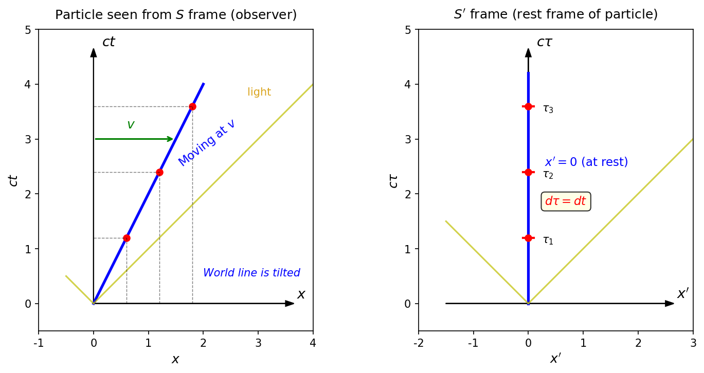
Fig. 4.4: Intuitive understanding of proper time. Left — As seen from the \(S\) frame (observer), the particle moves with velocity \(v\), so its worldline tilts. Right — As seen from the particle's own rest frame \(S'\), it always remains at the origin \(x' = 0\) and simply moves straight along the \(c\tau\) axis. This \(\tau\) is the proper time.
🟡 Lina: Look at the right side of Fig. 4.4 "Intuitive understanding of proper time. Left". In the particle's own rest frame \(S'\), the particle isn't moving—spatial coordinates are always zero, and only time advances. The "time ticked by its own clock" is the proper time \(\tau\).
⚪ Mei: I see—from the \(S\) frame the worldline tilts, but from the particle's own perspective it's just moving straight in the time direction—that time is \(\tau\).
🟡 Lina: Right. And the crucial point is that every observer uses this particle's proper time \(\tau\) to define quantities like velocity. The reason is that coordinate time \(t\) takes different values in different inertial frames, but proper time \(\tau\) is an invariant—it has the same value regardless of which inertial frame you calculate it from. Dividing by an invariant ensures the result is also an invariant (or a quantity that follows the correct transformation law).
🔵 Kai: "Dividing by an invariant ensures the result follows the correct transformation law"—can you be more specific about what that means?
🟡 Lina: For example, \(dx^\mu\) is a contravariant vector—a quantity that transforms by multiplying with \(\Lambda\) under Lorentz transformations. If we divide this by \(d\tau\) (a scalar, meaning a quantity whose value doesn't change under transformations), only the numerator transforms with \(\Lambda\) while the denominator is invariant, so the result \(dx^\mu / d\tau\) also follows the contravariant vector transformation law. If we divided by coordinate time \(dt\) instead, since \(dt\) itself changes between inertial frames, the result wouldn't be a contravariant vector.
⚪ Mei: That's why we need to divide by proper time \(\tau\) rather than coordinate time \(t\). To preserve the transformation law.
🟡 Lina: So, how do we define proper time mathematically? It's "the time in the particle's rest frame," so we want a quantity that equals \(d\tau = dt\) in the particle's rest frame (\(dx = dy = dz = 0\)). Moreover, it must be an invariant (giving the same value regardless of which inertial frame we calculate from)—otherwise the meaning of "the particle's own clock" would depend on the coordinate system.
🔵 Kai: An invariant… ah, \(ds^2\)?
🟡 Lina: Right. In Section 2 of Ch. 3, we showed that \(ds^2\) is an invariant that takes the same value in all inertial frames. It's the invariant that directly gives the "spacetime distance" between two nearby events from the infinitesimal coordinate displacements. So let's calculate \(ds^2\) in the particle's rest frame—the inertial frame moving along with the particle. In this frame, the particle isn't moving, so spatial coordinates don't change: \(dx = dy = dz = 0\). Substituting gives \(ds^2 = -dt^2 + 0 + 0 + 0 = -dt^2\). Here, "\(dt\) in the rest frame" is the time ticked by a clock moving with the particle—that is, a clock placed right next to the particle (in the right side of Fig. 4.4 "Intuitive understanding of proper time. Left", the time as the particle moves along the time axis without moving spatially). Since there's a minus sign, \(ds^2 < 0\). And since \(ds^2\) is an invariant, calculating \(ds^2 = -dt^2 + dx^2 + dy^2 + dz^2\) in another inertial frame gives the same numerical value—matching the \(-dt^2\) obtained in the rest frame.
🔵 Kai: \(ds^2\) is negative… that's the square of time but with a minus sign—is that OK?
🟡 Lina: Good question. That's exactly the key point. What we want to do is define "the time \(d\tau\) ticked by the particle's own clock"—we want a real number for time. So \(d\tau^2\) must be positive. But \(ds^2\) turns out negative. Why negative?—In the rest frame (\(dx = dy = dz = 0\)), \(ds^2 = -dt^2 < 0\). And since \(ds^2\) is an invariant, if it's negative in the rest frame, it's negative in every other inertial frame too.
🔵 Kai: So, for a particle moving slower than light, \(ds^2 < 0\) no matter which inertial frame you calculate in.
🟡 Lina: Exactly. We can verify this directly in a general inertial frame—the particle's speed is \(v^2 = (dx^2 + dy^2 + dz^2)/dt^2\), so if \(v < 1\) (subluminal), then \(v^2 < 1\). Multiplying both sides by \(dt^2 > 0\) gives \(dx^2 + dy^2 + dz^2 < dt^2\), hence \(ds^2 = -dt^2 + dx^2 + dy^2 + dz^2 < 0\).
Now, since \(ds^2 < 0\), we can't take the square root to get a real "time." The solution is simple—attach a minus sign so that \(-ds^2 > 0\). In the rest frame, \(-ds^2 = -(-dt^2) = dt^2\)—exactly "the square of the particle's own clock time." And since \(ds^2\) is an invariant, \(-ds^2\) is also an invariant. So we define proper time as
🔵 Kai: Just attaching a minus sign solves it. Sign conventions really matter!
🟡 Lina: With this definition, in the rest frame (\(dx = dy = dz = 0\)), \(d\tau^2 = dt^2\), i.e., \(d\tau = dt\)—properly corresponding to "the particle's own clock." And since \(ds^2\) is an invariant in all inertial frames (as we derived in Section 2 of Ch. 3), \(-ds^2\) is naturally also an invariant—we just flipped the sign. Therefore \(d\tau\) is an invariant, giving the same value no matter which inertial frame you calculate from.
🔵 Kai: I see—you worked backward from wanting \(d\tau = dt\) in the rest frame to construct the definition. Since \(ds^2\) is negative, you attach a minus sign to make it positive—and then \(d\tau\) is real.
🟡 Lina: Exactly.
Note: This definition gives \(d\tau^2 > 0\) only when \(ds^2 < 0\) (timelike), meaning \(d\tau\) is meaningful as a real number. In other words, proper time is defined only along worldlines of particles moving slower than light—paths that are causally accessible. Proper time cannot be defined for light (\(ds^2 = 0\)) or hypothetical superluminal paths.
⚪ Mei: In the particle's rest frame, \(dx = dy = dz = 0\) so \(d\tau = dt\). So proper time is "the time of a clock moving together with the particle."
🔵 Kai: Then what happens to \(d\tau\) as seen from the \(S\) frame where the particle is moving? Since \(dx \neq 0\), does \(d\tau < dt\)?
🟡 Lina: Exactly. In the \(S\) frame, the particle is moving so \(dx^2 + dy^2 + dz^2 > 0\), giving \(d\tau^2 = dt^2 - (dx^2 + dy^2 + dz^2) < dt^2\)—since \(d\tau > 0\) and \(dt > 0\) (moving forward in time), we get \(d\tau < dt\). The proper time of a moving particle is shorter than the coordinate time in the \(S\) frame. This is the same thing as "moving clocks run slow" that we saw in Section 4.2 of Ch. 3. Let me now calculate exactly how much shorter.
🟡 Lina: The definition of four-velocity is
\(d\tau\) is a scalar (invariant), and \(dx^\mu\) is a contravariant vector. As I explained earlier, since a scalar doesn't change under Lorentz transformations, the transformation law of \(dx^\mu / d\tau\) is that of the numerator \(dx^\mu\) alone—namely, the contravariant vector transformation law with one factor of \(\Lambda\). Therefore \(U^\mu\) is a contravariant vector.
🔵 Kai: What do the components look like specifically?
🟡 Lina: Let's follow the definition \(U^\mu = dx^\mu / d\tau\) and express each component in terms of coordinate time \(t\). First, we need to rewrite \(d\tau\) in terms of \(dt\). Taking the definition \(d\tau^2 = dt^2 - dx^2 - dy^2 - dz^2\) and factoring out \(dt^2\) from the right side:
The notation \(dx^2/dt^2\) here might be confusing, but it means \((dx)^2/(dt)^2 = (dx/dt)^2\)—the ratio of squares of infinitesimals equals the square of the derivative.
🔵 Kai: Um, what exactly does "factoring out \(dt^2\)" mean?
🟡 Lina: We divide all 4 terms on the right side of \(d\tau^2 = dt^2 - dx^2 - dy^2 - dz^2\) by \(dt^2\), then factor \(dt^2\) out front. \(dt^2/dt^2 = 1\), \(dx^2/dt^2 = (dx/dt)^2\), \(dy^2/dt^2 = (dy/dt)^2\), \(dz^2/dt^2 = (dz/dt)^2\). So \(d\tau^2 = dt^2\bigl(1 - (dx/dt)^2 - (dy/dt)^2 - (dz/dt)^2\bigr)\). Using the 3-dimensional speed squared \(v^2 \equiv (dx/dt)^2 + (dy/dt)^2 + (dz/dt)^2\) (with \(c = 1\) units, \(0 \le v < 1\)): $$ d\tau^2 = dt^2(1 - v^2) $$
Taking the square root (taking the positive root since \(dt > 0\) and \(d\tau > 0\)), \(d\tau = dt\sqrt{1 - v^2}\), meaning
🔵 Kai: Ah, \(\gamma\) appears! The ratio of proper time to coordinate time is exactly the Lorentz factor.
🟡 Lina: Right. So, converting the derivative with respect to \(\tau\) to a derivative with respect to \(t\) (using the chain rule \(dx^\mu/d\tau = (dx^\mu/dt)(dt/d\tau)\)):
Here \(v^i = dx^i/dt\) is the ordinary 3-dimensional velocity. The time component in the parentheses is 1 because \(dx^0/dt = dt/dt = 1\) (multiplied by \(\gamma\) gives \(U^0 = \gamma\)).
🔵 Kai: How do you calculate the "magnitude" of this \(U^\mu\)? In 3 dimensions it's \(|\vec{v}|^2 = v_x^2 + v_y^2 + v_z^2\), but...
🟡 Lina: In 4-dimensional spacetime, the quantity corresponding to the "magnitude squared" of a vector—called the norm—is calculated using the metric \(\eta_{\mu\nu}\). The analog of \(|\vec{v}|^2 = v_x^2 + v_y^2 + v_z^2\) in 3 dimensions is
Expanding using the summation convention from Section 1.3 gives \((-1)(U^0)^2 + (U^1)^2 + (U^2)^2 + (U^3)^2\). Unlike 3 dimensions, the time component has a minus sign, so the norm can take negative values—while "length squared" in 3 dimensions is always positive, in spacetime the sign carries physical meaning (timelike, spacelike, or lightlike). Try substituting \(U^\mu = \gamma(1, v^x, v^y, v^z)\).
⚪ Mei: Substituting:
🔵 Kai: The magnitude of the four-velocity is always \(-1\)! It's constant regardless of speed.
🟡 Lina: Yes. This property follows automatically from the definition of proper time. The norm being \(-1\) (negative) means the four-velocity is a timelike vector—that is, a vector satisfying \(\eta_{\mu\nu} V^\mu V^\nu < 0\). We're applying the same classification from Section 2.3 of Ch. 3 (where we called intervals with \(ds^2 < 0\) "timelike") to vectors—if the norm of a vector is negative, it's timelike; if zero, lightlike; if positive, spacelike. Timelike vectors point inside the light cone.
🔵 Kai: If the norm is constant at \(-1\), does that mean you can't change the "magnitude" of the four-velocity?
🟡 Lina: Correct. Intuitively, here's what it means—in the particle's rest frame, \(U^\mu = (1, 0, 0, 0)\). That is, the particle is moving at "speed 1" (= the speed of light) in the time direction. It's not moving in any spatial direction.
⚪ Mei: From another inertial frame, \(U^\mu = \gamma(1, v, 0, 0)\) and spatial components appear. But the norm stays \(-1\).
🟡 Lina: Right. The four-velocity vector just tilts in the \(t\)-\(x\) plane while preserving its norm (magnitude)—the same structure as the hyperbolic rotation we saw in Section 3.7 of Ch. 3. The faster you move in the spatial direction, the larger the time component \(\gamma\) grows, maintaining the norm at \(-1\).
🔵 Kai: …So the faster you move spatially, the larger the time component grows to keep the norm fixed. I get this image that everyone is moving through spacetime at "the speed of light," and the only difference is whether that direction is more time-like or space-like—is that correct?
🟡 Lina: That's an interesting intuition. But be careful—"moving at the speed of light" is just a metaphor; precisely, it means "the norm of the four-velocity is \(-1\) (or \(-c^2\) when restoring \(c\)) and constant." A photon's norm is 0, so massive particles and photons aren't "moving at the speed of light" in the same sense. This metaphor is often used in popular science books, but it slightly diverges from the mathematical meaning, so you might lose points if you wrote it on an exam (laughs).
🔵 Kai: Then how should you state it precisely?
🟡 Lina: Precisely stated—the norm of the four-velocity of all massive particles cannot be changed. Moving faster spatially causes the time component \(U^0 = \gamma\) to grow correspondingly, maintaining the norm at \(-1\). As a result, proper time advances more slowly—this is the four-velocity reformulation of "moving clocks run slow" from Section 4.2 of Ch. 3.
🔵 Kai: Then what about photons? With zero mass, \(d\tau\) in \(U^\mu = dx^\mu/d\tau\) becomes zero, so it can't be defined, right?
🟡 Lina: Sharp. That's exactly right—proper time cannot be defined for photons (since \(ds^2 = 0\) means \(d\tau = 0\)). So four-velocity can't be used for photons. Then how do we describe photon motion?—We'll address that in "Massless Particles" after introducing four-momentum.
✅ Comprehension Check: Why do we differentiate with respect to proper time \(\tau\) rather than coordinate time \(t\) in the definition of four-velocity?
Answer
Coordinate time \(t\) takes different values in different inertial frames, but proper time \(\tau\) is an invariant (giving the same value regardless of which inertial frame you calculate from). Dividing by an invariant guarantees that the result obeys the correct transformation law (the contravariant vector transformation law).
Four-Momentum¶
🟡 Lina: Once we have four-velocity, we can naturally define four-momentum \(p^\mu\).
Here \(m\) is the particle's (rest) mass.
🔵 Kai: The spatial components \(p^i = \gamma m v^i\) are… ah, at low speeds \(\gamma \approx 1\) so it reduces to Newton's momentum \(mv^i\). Then what does the time component \(p^0 = \gamma m\) represent?
🟡 Lina: In the \(c = 1\) unit system, \(p^0 = \gamma m = E\)—it equals the energy. To convert back to SI units, we use the dimensional analysis from Section 1.1. The spatial components \(p^i = \gamma m v^i\) of \(p^\mu = (p^0, p^1, p^2, p^3)\) have the dimensions of momentum \([\text{kg}\cdot\text{m/s}]\).
🔵 Kai: Does the time component \(p^0\) need to have the same dimensions?
🟡 Lina: Yes. When you expand the Lorentz transformation \(p^{\mu'} = \Lambda^{\mu'}{}_{\nu} p^\nu\), the right side becomes a sum of \(p^0, p^1, p^2, p^3\). For addition to make sense, all components must have the same dimensions—you can't add "3 kg·m/s + 5 joules."
🔵 Kai: Right, you can only add quantities of the same dimension.
🟡 Lina: Exactly. In SI, the spatial components \(p^i = \gamma mv^i\) (\(v^i\) has dimensions of m/s) have momentum dimensions \([\text{kg}\cdot\text{m/s}]\). So the time component must have the same dimensions. In natural units \(p^0 = \gamma m\), but what happens when converting back to SI? Let's use the dimensional analysis from Section 1.1. In natural unit expressions where \(c = 1\) was set and \(c\) disappeared, we restore it. The dimensions of \(\gamma m\) are \([\text{kg}]\), which is missing \([\text{m/s}]\) compared to the spatial component dimensions \([\text{kg}\cdot\text{m/s}]\). So we supplement with \(c\) (dimensions \([\text{m/s}]\)), giving the correct SI expression \(p^0 = \gamma mc\)—now it's \([\text{kg}\cdot\text{m/s}]\). Meanwhile, the SI expression for energy is \(E = \gamma mc^2\) (dimensions: \([\text{kg}\cdot\text{m}^2/\text{s}^2]\)). Then \(E/c = \gamma mc\) (dimensions: \([\text{kg}\cdot\text{m/s}]\))—the same dimensions as the spatial components. So in SI units, writing \(p^0 = E/c\) makes all component dimensions match.
Note: Some textbooks define the time coordinate from the start as \(x^0 = ct\) (with length dimensions) to make all component dimensions uniform. In that case \(U^0 = dx^0/d\tau = c\,dt/d\tau = \gamma c\), \(p^0 = mU^0 = \gamma mc = E/c\), and the conclusion is the same. Since this chapter unifies everything with \(c = 1\), we can simply write \(p^0 = E\).
To summarize—in this chapter (\(c = 1\)), \(p^0 = E\). Converting back to SI gives \(p^0 = E/c\). When you need specific numerical values in SI, restore \(c\) using the dimensional analysis from Section 1.1. Expanding at low speed gives \(E \approx m + \frac{1}{2}mv^2\) (\(c = 1\)); restoring \(c\) gives \(E \approx mc^2 + \frac{1}{2}mv^2\)—the sum of rest energy and kinetic energy. The derivation of this expansion is done in detail in the upcoming "Low-Speed Limit and Connection to Newtonian Mechanics".
🟡 Lina: Let's compute the invariant norm of the four-momentum. Since \(p^\mu = mU^\mu\):
In components: \(-(p^0)^2 + |\vec{p}|^2 = -m^2\). With \(c = 1\) and \(p^0 = E\): \(-E^2 + |\vec{p}|^2 = -m^2\), giving \(E^2 = |\vec{p}|^2 + m^2\). This is the energy-momentum relation in \(c = 1\) units.
🔵 Kai: Wow, the energy-momentum relation comes out just from the invariance of the norm!
🟡 Lina: To restore \(c\), use the dimensional analysis from Section 1.1. In the \(c = 1\) expression \(E^2 = |\vec{p}|^2 + m^2\), each term has different SI dimensions—the left side \(E^2\) is energy squared with dimensions \([\text{kg}^2\cdot\text{m}^4/\text{s}^4]\), \(|\vec{p}|^2\) is momentum squared with dimensions \([\text{kg}^2\cdot\text{m}^2/\text{s}^2]\), and \(m^2\) is mass squared with dimensions \([\text{kg}^2]\). To match each term to the left side's dimensions \([\text{kg}^2\cdot\text{m}^4/\text{s}^4]\)—\(|\vec{p}|^2\) is missing \([\text{m}^2/\text{s}^2]\) so multiply by \(c^2\), and \(m^2\) is missing \([\text{m}^4/\text{s}^4]\) so multiply by \(c^4\). Therefore:
⚪ Mei: From the invariance of the norm, the energy-momentum relation comes out in one shot.
🔵 Kai: When \(\vec{p} = 0\) (at rest), \(E^2 = m^2 c^4\), i.e., \(E = mc^2\)—so \(E = mc^2\) was just a special case of this equation! But wait a moment. If I put in \(m = 0\), I get \(E = |\vec{p}|c\), meaning something with zero mass can still have energy? Isn't that strange?
🟡 Lina: Good question. That's right—zero mass doesn't mean zero energy and momentum. Photons are exactly like this. We'll cover this in more detail in Section 2.7, so hang on a moment.
🔵 Kai: Also, you mentioned earlier that "expanding at low speed gives \(E \approx m + \frac{1}{2}mv^2\)." I intuitively understand that Newton's kinetic energy should appear, but I'm curious how that approximation comes from \(\gamma m\). And what is four-momentum actually useful for? In Newtonian mechanics, momentum conservation and energy conservation were separate laws, but…
🟡 Lina: The low-speed expansion derivation is a good question—we'll do it carefully in the next section ("Low-Speed Limit and Connection to Newtonian Mechanics"), so hold on. Let me first answer "what four-momentum is useful for." Consider particle collisions or decays, for example. When two particles collide and produce new particles, \(p^\mu_{\text{total}}\) is conserved before and after the reaction—meaning energy and momentum are conserved simultaneously. In Newtonian mechanics, momentum conservation and energy conservation were separate laws, but in relativity where time and space are unified, they become conservation of a single four-vector, the four-momentum \(p^\mu = (E, \vec{p})\).
🔵 Kai: Two separate laws in Newtonian mechanics get unified into one equation in relativity…. But wait, in Newtonian mechanics, momentum conservation came from Newton's third law (action-reaction). In relativity, the third law can't be used directly, so where does four-momentum conservation come from?
🟡 Lina: Good question. In Section 5 of Ch. 1, we saw the relationship between "symmetries and conserved quantities"—time translation symmetry guarantees energy conservation, and spatial translation symmetry guarantees momentum conservation. In relativity, where time and space are unified, these two conservation laws become unified as four-momentum conservation from spacetime translation symmetry. The rigorous derivation will be revisited in later chapters in the context of field theory.
✅ Comprehension Check: From \(E^2 = |\vec{p}|^2 c^2 + m^2 c^4\), what conclusion can we draw about massless particles (photons)?
Answer
Substituting \(m = 0\) gives \(E = |\vec{p}|c\), meaning even a massless particle can have energy and momentum. Furthermore, the speed of a massive particle is given by \(v = |\vec{p}|c^2/E\) (derivable from \(\vec{p} = \gamma m\vec{v}\) and \(E = \gamma mc^2\)). In the \(m \to 0\) limit, substituting \(E = |\vec{p}|c\) gives \(v = |\vec{p}|c^2/(|\vec{p}|c) = c\), so massless particles always travel at the speed of light.
Low-Speed Limit and Connection to Newtonian Mechanics¶
🔵 Kai: Earlier, Lina, you just stated the conclusion that "expanding at low speed gives \(E \approx mc^2 + \frac{1}{2}mv^2\)." How do you actually derive this?
🟡 Lina: Good focus. Let's actually calculate it. We just need to approximate \(\gamma\) in \(E = \gamma mc^2\) for \(v \ll c\). Applying the approximation formula \((1 + x)^n \approx 1 + nx\) (for \(|x| \ll 1\)) learned in high school, with \(x = -v^2/c^2\) and \(n = -1/2\):
Substituting into \(E = \gamma mc^2\):
⚪ Mei: The first term is the rest energy, and the second term is Newton's kinetic energy. They separate cleanly.
🟡 Lina: Right. And the important point is that when \(v \ll c\), the second term is extremely small compared to the first. Even at \(v = 100\,\text{m/s}\) (slightly faster than a bullet train), \(v^2/c^2 \sim 10^{-13}\), so the kinetic energy is 13 orders of magnitude smaller than the rest energy \(mc^2\).
🔵 Kai: If it differs by 13 orders of magnitude, there's no way Newton's era could have noticed. But conversely, the fact that enormous energy is released when mass decreases by just a tiny amount in nuclear reactions—is that because this \(mc^2\) is so huge?
🟡 Lina: Exactly. In everyday motion, only \(\frac{1}{2}mv^2\) is visible, and the enormous \(mc^2\) behind it was completely hidden. Only when relativity revealed that "mass stores energy" could nuclear reactions—releasing enormous energy by liberating just a tiny fraction of \(mc^2\)—be understood.
Massless Particles¶
🟡 Lina: And one more important consequence. Putting a massless particle (photon) into \(E^2 = |\vec{p}|^2 c^2 + m^2 c^4\):
Even with zero mass, it can have energy and momentum. And to realize \(E = \gamma mc^2\) with \(m = 0\) and \(E \neq 0\), we need \(\gamma \to \infty\), meaning \(v = c\)—massless particles always travel at the speed of light. Photons, and gravitons (particles predicted theoretically but not yet discovered, which we'll discuss in Ch. 25), are all thought to satisfy this relation.
✅ Comprehension Check: What is the value of the invariant norm \(\eta_{\mu\nu} U^\mu U^\nu\) of the four-velocity \(U^\mu\)?
Answer
\(-1\) (in the \(c = 1\) unit system). It is always constant regardless of speed, and this follows automatically from the definition of proper time.
📝 Exercises:
- Normalization of four-velocity, low-speed limit of relativistic energy, four-acceleration → Problem B-7. Verification of the Four-Velocity Normalization Condition, Problem B-8. Low-Speed Limit of Relativistic Energy, Problem A-1. Four-Velocity and Four-Acceleration
4.3 Upper and Lower Indices — Covariant Vectors¶
Lowering Indices¶
🟡 Lina: So far we've been talking about \(A^\mu\) (upper indices), but we also need to introduce lower indices \(A_\mu\). The definition is
🔵 Kai: You contract with the metric \(\eta_{\mu\nu}\). What does this look like specifically?
🟡 Lina: Since \(\eta_{\mu\nu}\) is diagonal with \(\eta_{00} = -1\), \(\eta_{11} = \eta_{22} = \eta_{33} = 1\):
Similarly \(A_2 = A^2\), \(A_3 = A^3\). (When summing over \(\nu\), since \(\eta_{1\nu}\) is zero for \(\nu \neq 1\), only the single term \(\eta_{11}\,A^1\) survives.)
⚪ Mei: So only the time component flips sign, and the spatial components stay the same. If \(A^\mu = (A^0, A^1, A^2, A^3)\) then \(A_\mu = (-A^0, A^1, A^2, A^3)\).
🟡 Lina: Exactly. Let me illustrate this "raising and lowering of indices" in Fig. 4.5 "The operations of raising and lowering indices".
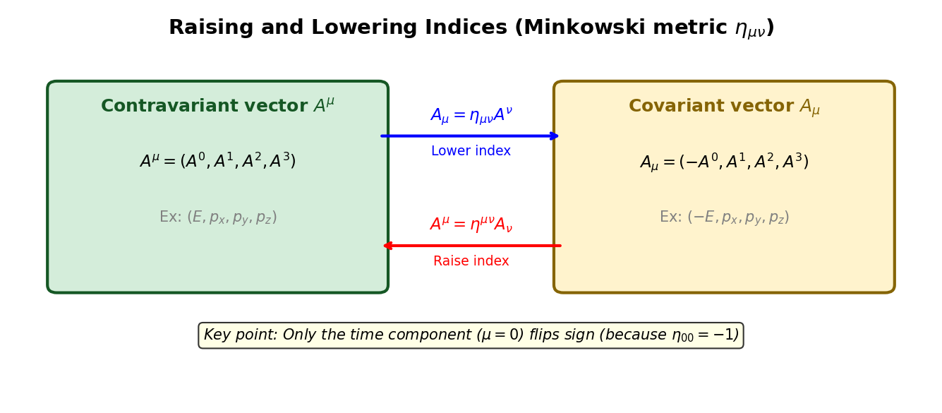
Fig. 4.5: The operations of raising and lowering indices. Multiplying by the metric \(\eta_{\mu\nu}\) creates the covariant vector \(A_\mu\) from the contravariant vector \(A^\mu\) (lowering the index). The inverse \(\eta^{\mu\nu}\) reverses the process (raising the index). For the Minkowski metric, only the time component flips sign.
🟡 Lina: \(A^\mu\) is called a contravariant vector, and \(A_\mu\) a covariant vector. The names "contravariant" and "covariant" come from the difference in how they transform under coordinate transformations.
Why two types of vectors are needed
Combining upper and lower indices and contracting yields a Lorentz-invariant scalar quantity. Using \(A_0 = -A^0\), \(A_i = A^i\) (\(i = 1, 2, 3\)) and actually expanding:
The minus sign on the time component remains because of the sign flip \(A_0 = -A^0\). This is invariant under Lorentz transformations. This structure of "combining upper and lower indices to form a scalar" is fundamental to calculations in general relativity.
⚪ Mei: Wait—the \(\eta_{\mu\nu}\,U^\mu\,U^\nu = -1\) we computed in Section 2.4, could that be related to this "lowering indices" operation?
🟡 Lina: Good observation. Exactly right. In \(\eta_{\mu\nu}\,U^\mu\,U^\nu\), \(\eta_{\mu\nu}\) lowers the index of \(U^\mu\) to form \(U_\nu = \eta_{\nu\mu} U^\mu\), and then takes the inner product with \(U^\nu\)—that is, \(U_\nu\,U^\nu = U_\mu\,U^\mu\). The notation differs but it's all the same calculation (since \(\eta_{\mu\nu} = \eta_{\nu\mu}\), the order of indices can be swapped).
Raising Indices¶
🟡 Lina: Conversely, to raise a lower index back to an upper one, use \(\eta^{\mu\nu}\) (the inverse matrix of \(\eta_{\mu\nu}\)).
For the Minkowski metric, \(\eta^{\mu\nu}\) is the same matrix as \(\eta_{\mu\nu}\) (diagonal components \(-1, 1, 1, 1\)).
🔵 Kai: Why are the inverse matrix and the original matrix the same?
🟡 Lina: \(\eta_{\mu\nu}\) is a diagonal matrix with diagonal entries \(-1, 1, 1, 1\). The inverse of a diagonal matrix is a diagonal matrix with the reciprocal of each diagonal entry. Since \((-1)^{-1} = -1\) and \(1^{-1} = 1\), the inverse has diagonal entries \(-1, 1, 1, 1\)—the same as the original. This is a special property of the Minkowski metric; for a general metric \(g_{\mu\nu}\), the inverse \(g^{\mu\nu}\) has different components from the original.
⚪ Mei: Being its own inverse—in a sense \(\eta_{\mu\nu}\) is a very easy-to-handle metric.
✅ Comprehension Check: When constructing the covariant vector \(A_\mu\) from the contravariant vector \(A^\mu = (A^0, A^1, A^2, A^3)\), which component's sign changes?
Answer
Only the time component flips sign. \(A_\mu = (-A^0, A^1, A^2, A^3)\). This is due to \(\eta_{00} = -1\) and \(\eta_{ii} = 1\).
4.4 Basics of Tensors¶
What Is a Tensor?¶
🟡 Lina: Now we enter the general discussion of tensors. In fact, four-vectors are "tensors with one index" (rank-1 tensors). Here we'll extend to rank-2 tensors with "two indices," understanding their transformation law and the mechanism of contraction.
🔵 Kai: \(\eta_{\mu\nu}\) also has two indices. Is that a tensor too?
🟡 Lina: Exactly. In Section 2.3, we said that a contravariant vector transforms as \(V^{\mu'} = \Lambda^{\mu'}{}_{\nu}\,V^\nu\)—one index, so one factor of \(\Lambda\). Now, how does a quantity \(T^{\mu\nu}\) with two indices transform? The answer is simple—one factor of \(\Lambda\) per index. Two indices means two factors of \(\Lambda\):
Let me illustrate the structure of this transformation law in Fig. 4.6 "Geometric picture of tensor coordinate transformations. Left: The same physical vector \(\mathbf{V}\) has different components depending on whether it's expanded in basis \(\mathbf{e}_i\) (blue) or \(\mathbf{e}'_i\) (red). Right: Transformation laws for contravariant, covariant, and rank-2 tensors".
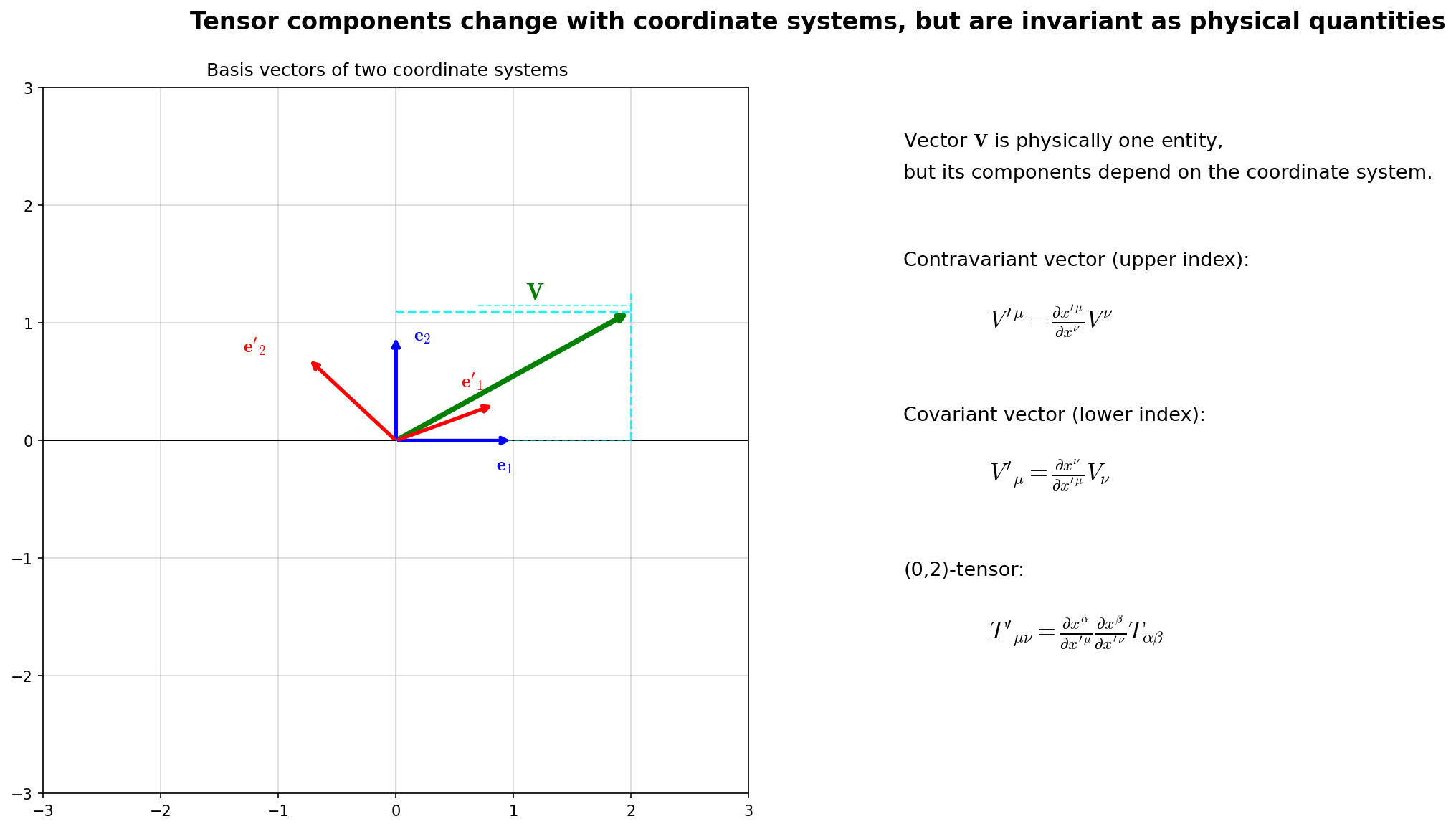
Fig. 4.6: Geometric picture of tensor coordinate transformations. Left: The same physical vector \(\mathbf{V}\) has different components depending on whether it's expanded in basis \(\mathbf{e}_i\) (blue) or \(\mathbf{e}'_i\) (red). Right: Transformation laws for contravariant, covariant, and rank-2 tensors—one transformation matrix (in special relativity the Lorentz transformation \(\Lambda\); in general, the coordinate transformation matrix \(\partial x'^\mu/\partial x^\nu\)) per index. Since the physical quantity itself is coordinate-independent, the component transformation law describes "how things shift when viewing the same object in different coordinates."
🔵 Kai: Ah, I see the pattern (the right side of Fig. 4.6 "Geometric picture of tensor coordinate transformations. Left: The same physical vector \(\mathbf{V}\) has different components depending on whether it's expanded in basis \(\mathbf{e}_i\) (blue) or \(\mathbf{e}'_i\) (red). Right: Transformation laws for contravariant, covariant, and rank-2 tensors" shows exactly this). Rank 1 (vector) gets one \(\Lambda\), rank 2 gets two. Rank 3 would get three…. So just like with vectors, the tensor itself is a coordinate-independent physical quantity, and only the components change with the choice of coordinates. But while I see the pattern, I can't quite picture what "two factors of \(\Lambda\)" means concretely. Could you show me the expansion?
✅ Comprehension Check: Why are two factors of \(\Lambda\) needed in the transformation law of a rank-2 tensor \(T^{\mu\nu}\)?
Answer
\(T^{\mu\nu}\) has two indices (\(\mu\) and \(\nu\)), and when changing inertial frames, each index needs to be transformed independently. One \(\Lambda\) for the first index and another \(\Lambda\) for the second, totaling two. With only one \(\Lambda\), only one index would be transformed, leaving things incomplete.
🟡 Lina: Sure. Let's unpack \(T^{\mu'\nu'} = \Lambda^{\mu'}{}_{\alpha}\,\Lambda^{\nu'}{}_{\beta}\,T^{\alpha\beta}\). First, \(\alpha\) and \(\beta\) are dummy indices (appearing both up and down, so we sum over them). This means the equation is shorthand for
A sum of \(4 \times 4 = 16\) terms.
🔵 Kai: For rank 1, \(V^{\mu'} = \sum_{\nu} \Lambda^{\mu'}{}_{\nu} V^\nu\) was a sum of 4 terms, so each additional index adds one more layer of summation.
🟡 Lina: Right. For example, if you want the \(\mu' = 0\), \(\nu' = 1\) component, you run \(\alpha\) and \(\beta\) each from 0 to 3 and sum all 16 terms. However, for an \(x\)-direction boost \(\Lambda\) (look at the matrix in "The Displacement Four-Vector"), components involving \(y, z\) directions vanish: \(\Lambda^{0'}{}_{2} = \Lambda^{0'}{}_{3} = \Lambda^{1'}{}_{2} = \Lambda^{1'}{}_{3} = 0\) (in rows \(\mu' = 0\) and \(\mu' = 1\), columns \(\nu = 2, 3\) are zero), so only the 4 terms with \(\alpha, \beta = 0, 1\) survive:
For a general Lorentz transformation (including rotations), all 16 terms may survive, but the structure is the same—think of it as "repeating the vector transformation twice."
🔵 Kai: So, if the values computed by applying two \(\Lambda\)'s to the \(S\) frame components \(T^{\alpha\beta}\) match the actually measured \(T^{\mu'\nu'}\) in the \(S'\) frame—that's what makes something a tensor?
🟡 Lina: Exactly. Same structure as Section 2.3 where we said "a quantity that gives the correct answer when \(\Lambda\) is applied is a contravariant vector." A quantity that gives the correct answer when two \(\Lambda\)'s are applied is a rank-2 contravariant tensor.
🔵 Kai: Why does \(\Lambda\) need to be applied twice? Why not just once?
🟡 Lina: \(T^{\mu\nu}\) has two indices. \(\mu\) and \(\nu\). When changing inertial frames, each index needs to be independently transformed. One \(\Lambda\) to transform the first index \(\mu\), another to transform the second index \(\nu\). So two total.
🔵 Kai: Ah, I see. If you only applied \(\Lambda\) once, one index would be transformed to the \(S'\) frame while the other remains in the \(S\) frame—a half-baked state. Can you show me a concrete example?
🟡 Lina: Sure. The most intuitive rank-2 tensor is formed by multiplying the components of two vectors in all combinations: \(T^{\mu\nu} = A^\mu B^\nu\). For example, \(T^{01} = A^0 B^1\), \(T^{23} = A^2 B^3\)—a quantity with \(4 \times 4 = 16\) components. In the \(S'\) frame, \(A^{\mu'} = \Lambda^{\mu'}{}_{\alpha} A^\alpha\) and \(B^{\nu'} = \Lambda^{\nu'}{}_{\beta} B^\beta\), so:
One \(\Lambda\) to transform \(A\), another to transform \(B\). Two in total. If you only applied \(\Lambda\) once, only \(A\) would be transformed to the \(S'\) frame while \(B\) stays in \(S\)—giving the meaningless quantity \(A^{\mu'} B^{\nu}\).
⚪ Mei: Thinking about it as a product of two vectors makes the reason for needing two \(\Lambda\)'s crystal clear.
🟡 Lina: A vector \(V^\mu\) has one index so needs \(\Lambda\) once. A tensor \(T^{\mu\nu}\) has two indices so needs it twice. Number of indices = number of \(\Lambda\)'s—this is the essence of tensor transformation laws. Quantities obeying this transformation law are called tensors, and the rank is determined by the number of indices.
Table 4.2: Correspondence between tensor rank, number of indices, and transformation law
| Rank | Number of indices | Number of \(\Lambda\)'s | Name | Examples |
|---|---|---|---|---|
| 0 | 0 | 0 | Scalar (invariant) | \(ds^2\), \(m\) |
| 1 | 1 | 1 | Four-vector | \(V^\mu\), \(U^\mu\), \(p^\mu\) |
| 2 | 2 | 2 | Rank-2 tensor | \(\eta_{\mu\nu}\), \(T^{\mu\nu}\) |
🔵 Kai: But why is this condition important?
🟡 Lina: For the same reason we discussed for vectors in Section 2.3. The numerical values of components change between inertial frames, but the physical content doesn't change. The transformation formula is "the conversion rule for components when viewing the same physical quantity from a different inertial frame." If you write equations using tensors, they take the same form in all inertial frames—this is the foundation of general relativity.
🔵 Kai: By the way, to say that \(\eta_{\mu\nu}\) is a tensor, what do we need to verify?
🟡 Lina: Strictly speaking, \(\eta_{\mu\nu}\) is a covariant tensor with two lower indices, so its transformation law differs slightly from the contravariant case—instead of \(\Lambda\), two factors of the inverse matrix \(\Lambda^{-1}\) appear. While contravariant tensors (upper indices) transform with \(\Lambda\), covariant tensors (lower indices) transform with \(\Lambda^{-1}\)—exactly the same structure as the relationship between contravariant and covariant vectors. The specific transformation formula and calculation are left to the exercises (→ Problem M-2. Metric Preservation Condition under Lorentz Transformation). The conclusion is that when you compute \(\eta_{\mu'\nu'}\), you get the same values as the original \(\eta_{\mu\nu}\)—meaning the Minkowski metric has the same components in all inertial frames. The reason why contravariant and covariant transformations go in opposite directions will be examined in detail in Section 4.4 where we see "\(\Lambda\) and \(\Lambda^{-1}\) cancel in upper-lower pairs." Here, let's look at the very special property that \(\eta_{\mu\nu}\) possesses.
\(\eta_{\mu\nu}\) Is the Same in All Inertial Frames¶
In the \(S\) frame:
In the \(S'\) frame, the same form holds due to the invariance of the speed of light:
🔵 Kai: In the \(S'\) frame too, the coefficients remain \((-1, 1, 1, 1)\)… meaning \(\eta_{\mu'\nu'}\) is also a matrix with diagonal entries \((-1, 1, 1, 1)\)—the same as in the \(S\) frame. But wait. Tensors are supposed to be "quantities whose components change under coordinate transformations," right? Components not changing—isn't that a contradiction?
🟡 Lina: Good question. First, a correction—the definition of a tensor is not "a quantity whose components change," but "a quantity that follows a specific transformation law." Following the transformation law and computing the result may produce changed components, or it may happen to produce the same values. \(\eta_{\mu\nu}\) is the latter case, and this isn't coincidental—it comes from the very definition of the Lorentz transformation. In Ch. 3, we defined the Lorentz transformation as "the transformation that preserves \(ds^2\)." If \(ds^2 = \eta_{\mu\nu}\,dx^\mu\,dx^\nu\) is invariant, that means it can be written with the same \(\eta\) components after transformation. In other words, the Minkowski metric components remain \((-1, 1, 1, 1)\) on the diagonal in all inertial frames—this is a property that necessarily follows from the definition of Lorentz transformations.
⚪ Mei: So since we defined Lorentz transformations as "transformations that preserve \(ds^2\)," it's automatic that the metric is invariant under those transformations—almost a tautology.
🟡 Lina: However, this is a property specific to special relativity (flat spacetime). In general relativity, the metric \(g_{\mu\nu}\) has components that change under coordinate transformations—that is the mathematical expression of "spacetime being curved."
Contraction — Summing Over Matched Upper and Lower Indices¶
🟡 Lina: Let me introduce an operation that will be used frequently in later chapters. An operation that lowers the rank of a tensor—called contraction.In Ch. 12, we'll create a rank-2 tensor from a rank-4 tensor, and then create a scalar—this "rank-lowering" operation is essential for constructing the Einstein equation.
🔵 Kai: Rank-4 tensors and such are still way ahead, right? Is this relevant to us now?
🟡 Lina: Actually, you've already used this operation—you just didn't know the name.
🔵 Kai: Huh, where?
🟡 Lina: The inner product from Section 3.1:
This is the most basic example of contraction. An upper index \(\mu\) (in \(B^\mu\)) and a lower index \(\mu\) (in \(A_\mu\)) appear as a pair, and we substitute \(\mu = 0, 1, 2, 3\) and add—this operation is called "contracting over \(\mu\)."
⚪ Mei: Ah, I see. So the Einstein summation convention we learned in Section 1.3 (omitting \(\sum\) when the same index appears up and down) is being reinterpreted as a meaningful operation.
🟡 Lina: Exactly. The notational rule (Section 1.3) and contraction as an operation (what we're doing now) refer to the same \(\sum\) calculation, but the perspectives differ—the former is "a convention for writing," the latter is "an operation on tensors."
Terminology note: 'summation convention' vs. 'contraction'
- Einstein summation convention: A notational agreement to omit \(\sum\)
- Tensor contraction: An operation that lowers rank by pairing upper and lower indices and summing
The names are similar, but one is about notation and the other is about operations. However, the computational content is the same \(\sum\).
Case of Two Vectors (Inner Product)¶
🟡 Lina: Let's visualize what contraction does in the inner product \(A_\mu B^\mu\). As index \(\mu\) runs from 0, 1, 2, 3, there are \(4 \times 4 = 16\) possible combinations of components of \(A\) and \(B\):
The contraction \(A_\mu B^\mu\) is the operation of selecting only the 4 "diagonal" entries (underlined) from these 16 combinations and adding them:
🔵 Kai: You select only 4 out of 16 and add them. It's like extracting the diagonal.
Case of a Rank-2 Tensor¶
🟡 Lina: Next, let's extend to rank-2 tensors. For \(T^\mu{}_\nu\) (2 indices, 16 components), if we set \(\nu\) to the same letter as \(\mu\) and write \(T^\mu{}_\mu\)—the same \(\mu\) appears up and down, so by the summation convention from Section 1.3, we sum:
Running \(\mu\) through 0, 1, 2, 3 and adding just the 4 diagonal components. This is simply the trace of the matrix.
⚪ Mei: The structure is exactly the same as in the inner product case. The subject changed from "vector \(A\) and vector \(B\)" to "one rank-2 tensor \(T\)," but the operation of "running an upper-lower index pair and summing" is the same.
🟡 Lina: Right. The operation itself can be unified. Let's dig a bit deeper into this unified perspective.
General Definition of Contraction¶
Contraction: When a tensor has one upper index and one lower index available, setting both to the same letter and substituting 0, 1, 2, 3 while summing. One pair of upper-lower indices disappears, so the rank decreases by two.
Table 4.3: Concrete examples of contraction and resulting ranks
| Original tensor | Contraction notation | Result |
|---|---|---|
| \(A_\mu\) and \(B^\mu\) (two vectors) | \(A_\mu B^\mu\) | Scalar (rank 0) = inner product |
| \(T^\mu{}_\nu\) (one rank-2 tensor) | \(T^\mu{}_\mu\) | Scalar (rank 0) = trace |
| \(R^\rho{}_{\sigma\mu\nu}\) (rank-4 tensor, appears in Ch. 12) | \(R^\mu{}_{\sigma\mu\nu} = R_{\sigma\nu}\) | Rank-2 tensor (Ricci tensor) |
🔵 Kai: Even though it's just "adding over index pairs," it gets different names—"inner product," "trace," "Ricci tensor"—depending on what you're applying it to.
🟡 Lina: The names differ for historical reasons, but the operation is unified. This is the strength of index notation—you can apply the same contraction rule to any tensor.
The Contraction Rule: Why It Must Be an Upper-Lower Pair¶
🔵 Kai: One question. You say we form pairs with upper and lower indices, but why can't we pair upper-with-upper or lower-with-lower? For example, summing \(A^\mu B^\mu\) with "both upper" would give the same thing, wouldn't it—
🟡 Lina: That doesn't work. The reason is that the result wouldn't be a scalar—meaning its value would change when you switch inertial frames.
Let's see this concretely. As we learned in Section 3.1, the relationship between upper and lower components is \(A_\mu = \eta_{\mu\nu} A^\nu\), with only the time component flipping sign: \(A_0 = -A^0\), \(A_i = A^i\). So if you forcefully summed \(A^\mu B^\mu\) with both indices up over \(\mu = 0, 1, 2, 3\):
On the other hand, the correct contraction \(A_\mu B^\mu\) gives:
Only the time component has a minus sign. This minus sign is the key to Lorentz invariance.
⚪ Mei: Wait. Why does that minus sign relate to Lorentz invariance?
🟡 Lina: Let's think about spatial rotations and boosts separately.
- Spatial rotations: The time components \(A^0, B^0\) don't change; only the 3 spatial components mix. Just like the Pythagorean theorem, \(A^i B^i = A^1 B^1 + A^2 B^2 + A^3 B^3\) is invariant under rotations.
- Boosts: The time axis and a spatial axis (say the \(x\) axis) mix together (the hyperbolic rotation from Section 3.7 of Ch. 3).
🔵 Kai: How do you verify that \(-A^0 B^0 + A^1 B^1\) is invariant under boosts?
🟡 Lina: As we saw in Section 3.7 of Ch. 3, a boost using rapidity \(\varphi\) (\(\tanh\varphi = v\)) takes the form \(t' = t\cosh\varphi - x\sinh\varphi\), \(x' = -t\sinh\varphi + x\cosh\varphi\). The same transformation applies to the contravariant vector \(A^\mu\): \(A^{0'} = A^0\cosh\varphi - A^1\sinh\varphi\), \(A^{1'} = -A^0\sinh\varphi + A^1\cosh\varphi\) (similarly for \(B^\mu\)). Omitting the \(y, z\) components which don't change, we want to verify that \(A_\mu B^\mu = -A^0 B^0 + A^1 B^1\) is invariant. Substituting into \(-A^{0'}B^{0'} + A^{1'}B^{1'}\) after transformation, the \(A^{0'}B^{0'}\) part is for instance
Similarly expanding \(A^{1'}B^{1'} = (-A^0\sinh\varphi + A^1\cosh\varphi)(-B^0\sinh\varphi + B^1\cosh\varphi)\) and computing \(-A^{0'}B^{0'} + A^{1'}B^{1'}\): the \(A^0 B^0\) terms give \(-\cosh^2\varphi + \sinh^2\varphi = -(\cosh^2\varphi - \sinh^2\varphi) = -1\) times, the \(A^1 B^1\) terms give \(-\sinh^2\varphi + \cosh^2\varphi = +(\cosh^2\varphi - \sinh^2\varphi) = +1\) times, and the cross terms (containing \(A^0 B^1\) or \(A^1 B^0\)) give \(+\cosh\varphi\sinh\varphi - \cosh\varphi\sinh\varphi = 0\), canceling—all thanks to the identity \(\cosh^2\varphi - \sinh^2\varphi = 1\) from Section 3.6 of Ch. 3. The result is \(-A^0 B^0 + A^1 B^1\)—the same as before. The full expansion calculation can be verified in the exercise → Problem A-2. General Direction Lorentz Boost.
🔵 Kai: So \(\cosh^2 - \sinh^2 = 1\) combined with "the minus sign on time" guarantees the invariance.
🔵 Kai: Conversely, what happens if you use all plus signs like \(A^0 B^0 + A^1 B^1 + \cdots\)?
🟡 Lina: Under a boost, \(\cosh^2\varphi + \sinh^2\varphi \neq 1\), so the value changes. The minus sign on the time component has the same origin as the sign pattern in \(ds^2 = -c^2 dt^2 + dx^2 + \cdots\)—it's the very nature of the Minkowski metric.
🔵 Kai: It's the same mechanism as \(ds^2\) from Section 2 of Ch. 3. The different signs for time and space are what guarantee the invariance of the speed of light…. So if the universe were Euclidean (all plus signs), would we not need the upper-lower distinction at all?
🟡 Lina: Sharp. That's correct—if the metric were the identity matrix \(\delta_{\mu\nu}\) (all plus signs), there would be no need to distinguish upper and lower, and \(A^\mu B^\mu\) would already be invariant. The reason the upper-lower distinction is necessary in Minkowski spacetime is precisely because time and space have different signs. More generally, writing the Lorentz transformation as \(\Lambda\) and its inverse as \(\Lambda^{-1}\):
- Upper-index vectors \(B^\mu\) transform with \(\Lambda\): \(B^{\mu'} = \Lambda^{\mu'}{}_{\nu} B^\nu\)
- Lower-index vectors \(A_\mu\) transform with \((\Lambda^{-1})^T\): \(A_{\mu'} = (\Lambda^{-1})^{\nu}{}_{\mu'} A_\nu\)
The specific index-carrying transformation formulas will be derived in later chapters; for now just remember "contravariant vectors transform with \(\Lambda\) while covariant vectors transform with the transpose of the inverse of \(\Lambda\)—meaning they undergo the opposite transformation."
🔵 Kai: \(\Lambda\) and \(\Lambda^{-1}\) transform in opposite directions… so when you pair upper and lower and multiply, the transformations cancel?
🟡 Lina: Exactly. The intuitive reason is this—\(A_\mu B^\mu\) is a scalar (invariant) with the same structure as the spacetime interval, so if \(B^\mu\) transforms with \(\Lambda\), then \(A_\mu\) must transform with the inverse of \(\Lambda\) for the product to be invariant. In a numerical analogy, it's like "\(2 \times \frac{1}{2} = 1\)"—they need to cancel. More concretely—when \(B^{\mu'} = \Lambda^{\mu'}{}_{\nu} B^\nu\) mixes the components of \(B\), \(A_{\mu'}\) mixes in the opposite way, so that when multiplied and summed (contracted), the effects of \(\Lambda\) cancel. So combining as an upper-lower pair \(A_\mu B^\mu\) makes the transformation matrices cancel, giving a scalar (invariant). With both upper, \(\Lambda\) gets applied twice without canceling; with both lower, the inverse matrix gets applied twice without canceling—in either case the value changes under Lorentz transformations.
Why contravariant (upper) and covariant (lower) transform in opposite directions
Intuitively, consider a transformation that makes the coordinate \(dx^\mu\) (upper index) "twice as large." For the covariant vector \(A_\mu\) representing the same physical quantity, its components must become "half as large" so that the inner product \(A_\mu\,dx^\mu\) maintains the same value. Therefore \(dx^\mu\) and \(A_\mu\) transform in opposite directions. For rigorous derivation, see references (e.g., Ishii, Understanding General Relativity Step by Step with Equations, §3).
⚪ Mei: So the "upper-lower pair" contraction rule is not merely a notational convention but an essential requirement for guaranteeing Lorentz invariance as physics. The upper-lower distinction of indices has real meaning.
🟡 Lina: Yes. Index notation is a notation that compactly expresses the physical guarantee that "writing things this way automatically ensures Lorentz invariance"—this is why index notation is absolutely indispensable in relativistic calculations.
Unified Understanding of Inner Products and Contraction¶
⚪ Mei: So when Lina said earlier "you've already used this operation"—it was because the inner product \(A_\mu B^\mu\) is precisely a contraction—both are "selecting only the 4 entries where upper and lower indices match and adding." But the inner product operates on "2 vectors" while the trace operates on "1 tensor"—can we really call them the same?
🟡 Lina: Good question. Actually, if you multiply all component combinations of two vectors \(A_\mu\) and \(B^\nu\), you get a rank-2 tensor with \(4 \times 4 = 16\) components—this is called a tensor product. Written as \(A_\mu B^\nu\), the \((\mu, \nu) = (0, 1)\) component is \(A_0 B^1\), listing all combinations. Same structure as "\(T^{\mu\nu} = A^\mu B^\nu\)" that Kai saw in "What Is a Tensor?"—we confirmed it satisfies the transformation law then. Summing the diagonal components (contracting with \(\mu = \nu\)) gives the inner product \(A_\mu B^\mu\). So it just looks different; the operation is unified.
🔵 Kai: I see—tensor product → contraction gives the inner product. Everything is connected.
🟡 Lina: In general, one contraction of a rank-\(n\) tensor gives a rank-\((n-2)\) tensor:
- Inner product: rank \(1 + 1 = 2\) → after contraction: 0 (scalar)
- Trace of rank-2 tensor: rank \(2\) → after contraction: 0 (scalar)
- Riemann tensor → Ricci: rank \(4\) → after contraction: 2
- Ricci → scalar curvature: rank \(2\) → after contraction: 0
This mechanism of "lowering the rank by 2" will be crucial in Ch. 12 when constructing scalar curvature from the curvature tensor.
✅ Comprehension Check: State in one sentence why contraction must be between an "upper index and a lower index pair."
Answer
When contracting over an upper-lower pair, the transformation matrix \(\Lambda\) and inverse matrix \(\Lambda^{-1}\) cancel each other to produce a Lorentz invariant (scalar). With both upper or both lower, they don't cancel, and the value changes when switching inertial frames.
📝 Exercises:
- Tensor contraction, general Lorentz boost, invariance of the Minkowski metric → Problem M-1. Tensor Contraction and Classification of Indices, Problem A-2. General Direction Lorentz Boost, Problem M-2. Metric Preservation Condition under Lorentz Transformation
4.5 Summary — The Full Picture of Minkowski Spacetime¶
🟡 Lina: Let's organize the framework we've built in this chapter.
⚪ Mei: The starting point was two postulates—the principle of relativity and the invariance of the speed of light. From these, the spacetime interval
was shown to be invariant.
🔵 Kai: The coordinate transformation preserving this invariant is the Lorentz transformation. Same structure as spatial rotations being "distance-preserving transformations."
🟡 Lina: And if we write physical models using quantities that transform correctly under Lorentz transformations—four-vectors and tensors—the equations take the same form in all inertial frames. This is covariance.
⚪ Mei: Let me organize the tools we've acquired in this chapter—
Table 4.4: Summary of basic tools in special relativity
| Tool | Content |
|---|---|
| Spacetime interval \(ds^2\) | \(-dt^2 + dx^2 + dy^2 + dz^2\). A scalar invariant in all inertial frames |
| Lorentz transformation | Coordinate transformation preserving \(ds^2\). \(t' = \gamma(t - vx)\), \(x' = \gamma(x - vt)\) |
| Minkowski metric \(\eta_{\mu\nu}\) | Matrix with diagonal entries \((-1, 1, 1, 1)\). The "distance measurement rule" for flat spacetime |
| Four-vector \(A^\mu\) | Quantity obeying \(A^{\mu'} = \Lambda^{\mu'}{}_{\nu}A^\nu\) under Lorentz transformations |
| Four-velocity \(U^\mu\) | \(\gamma(1, v^x, v^y, v^z)\). Invariant norm \(U_\mu U^\mu = -1\) |
| Four-momentum \(p^\mu\) | \((E, \vec{p})\). Invariant norm \(p_\mu p^\mu = -m^2\). $E^2 = |
| Raising/lowering indices | \(A_\mu = \eta_{\mu\nu}A^\nu\). Time component sign flips |
| Einstein summation convention | Same index up and down → sum (omit \(\sum\)) |
⚪ Mei: The Minkowski metric \(\eta_{\mu\nu}\) is the metric of flat spacetime. As Lina mentioned in Section 1, in general relativity this gets replaced by a position-dependent \(g_{\mu\nu}\).
🟡 Lina: Right. And that is the mathematical expression of "spacetime being curved." In the next chapter, we'll discuss the equivalence of acceleration and gravity—the equivalence principle—and open the path to understanding "why the metric varies from place to place."
Preview of the Next Chapter¶
In Ch. 5, we take up Einstein's equivalence principle. Titled "The Equivalence Principle — The Equivalence of Acceleration and Gravity," we use the elevator thought experiment to understand that "acceleration and a gravitational field are locally indistinguishable," and see how this is the first step toward "the spacetime metric \(g_{\mu\nu}\) varying from place to place"—that is, spacetime being curved.
References¶
- Hartle, J. B. Gravity: An Introduction to Einstein's General Relativity, Chapters 4–5. Addison-Wesley, 2003.
- Schutz, B. F. A First Course in General Relativity, 3rd ed., Chapters 1–3. Cambridge University Press, 2022.
- Sato, K. Relativity (Iwanami Kiso Butsuri Series), Chapters 1–5. Iwanami Shoten, 1996.
- Ishii, T. Understanding General Relativity Step by Step with Equations, Chapters 8–9. Beret Publishing, 2013.
- Lancaster, T. and Blundell, S. J. General Relativity for the Gifted Amateur, Chapters 1–2. Oxford University Press, 2014.
Feedback on this page
Let us know if something was unclear, incorrect, or could be improved.