Chapter 6: Quantization of the Electromagnetic Field — The Struggle with Gauge Freedom
Story so far:
In Ch. 5, we quantized the Dirac field and confirmed that the fermionic anticommutation relations \(\{a_{\mathbf{p},s}, a_{\mathbf{q},r}^\dagger\} = (2\pi)^3 \delta^3(\mathbf{p} - \mathbf{q})\delta_{sr}\) naturally realize the spin-statistics theorem, and that antiparticles emerge as positive-energy solutions. This completed the quantization of spin 0 (scalar field) and spin 1/2 (Dirac field).
Goals of this chapter
- Quantize the electromagnetic field (spin 1) and understand how gauge symmetry—a "redundancy in description"—causes serious difficulties for quantization
- Overcome these difficulties using two prescriptions, Coulomb gauge and Lorenz gauge, and ultimately derive that physical photons have only 2 transverse polarizations
6.1 The Lagrangian of the Maxwell Field—Starting Point
🟡 Lina: So we've quantized the scalar field and the Dirac field. The remaining protagonist is the photon—a spin-1 particle. Photons emerge when we quantize the electromagnetic field. But here, a fundamental difficulty awaits that wasn't present in the previous two cases.
🔵 Kai: What kind of difficulty?
🟡 Lina: To understand that, let's start by writing down the Lagrangian of the electromagnetic field. As we learned in Ch. 3, field theory begins with the Lagrangian density \(\mathcal{L}\). For the electromagnetic field, the free field without sources (charges or currents) is
The coefficient \(-1/4\) is a normalization constant chosen so that the correct Maxwell equations emerge from the Euler-Lagrange equations—we'll verify this shortly. \(F_{\mu\nu}\) is called the field strength tensor, defined as
\(A_\mu\) is the four-potential.
🔵 Kai: What components does \(A_\mu\) have?
🟡 Lina: It's a four-vector with 4 components.
\(A_0\) corresponds to the electric potential (scalar potential) you learned in high school, and \(\mathbf{A} = (A^1, A^2, A^3)\) (contravariant components) is the vector potential. Note that under the metric \(\eta_{\mu\nu} = \mathrm{diag}(+1,-1,-1,-1)\), we have \(A^i = -A_i\) (spatial components flip sign between upper and lower indices. In this chapter, we'll use contravariant components \(A^i\) when expressing physical electric and magnetic fields, and covariant components \(A_i\) in canonical formalism discussions). The electric field \(\mathbf{E}\) and magnetic field \(\mathbf{B}\) are given by
(We're using natural units \(c = 1\), so this is the form obtained from the Gaussian unit expression \(\mathbf{E} = -\nabla\Phi - \frac{1}{c}\frac{\partial\mathbf{A}}{\partial t}\) with \(c\) removed.) In other words, the electric and magnetic fields are "secondary quantities" derived from \(A_\mu\). Looking at definition (6.2), swapping \(\mu\) and \(\nu\) reverses the order of subtraction, so \(F_{\mu\nu} = -F_{\nu\mu}\)—it's an antisymmetric tensor. The diagonal components \(F_{\mu\mu}\) are automatically zero.
⚪ Mei: I see, antisymmetric with zero diagonal means the independent components are just the upper triangular part... \(4 \times 3 / 2 = 6\) of them.
🟡 Lina: Right. And those 6 correspond exactly to the 3 components of the electric field and 3 components of the magnetic field.
🟡 Lina: Yes. Writing out \(F^{\mu\nu} = \eta^{\mu\alpha}\eta^{\nu\beta}F_{\alpha\beta}\) explicitly gives
🔵 Kai: How do you derive the components of this matrix? For example, why does \(F^{0i} = -E_i\)?
🟡 Lina: Let's go through it step by step. First, we compare \(F_{0i} = \partial_0 A_i - \partial_i A_0\) with equation (6.3). In equation (6.3), \(\mathbf{A}\) refers to the physical vector potential, meaning the contravariant components \(A^i\). To lower the index, we use the metric: \(A_i = \eta_{ij}A^j = (-\delta_{ij})A^j = -A^i\) (spatial components flip sign due to the minus in the metric). Since \(A_i = -A^i\),
(Let's verify. Since \(A_i = -A^i\), we have \(\partial_0 A_i = -\partial_0 A^i\). Therefore \(F_{0i} = \partial_0 A_i - \partial_i A_0 = -\partial_0 A^i - \partial_i A_0\). Meanwhile, from equation (6.3), \(\nabla A_0\) is a vector whose components are \(\partial A_0/\partial x^i\), so \(E^i = -(\nabla A_0)_i - \dot{A}^i = -\partial_i A_0 - \partial_0 A^i\). Here \(\partial_i A_0 \equiv \partial A_0/\partial x^i\). Comparing the two confirms \(F_{0i} = E^i\).) Next, we raise the indices. Using \(F^{\mu\nu} = \eta^{\mu\alpha}\eta^{\nu\beta}F_{\alpha\beta}\) to find \(F^{0i}\), with the diagonal metric, for \(\mu = 0\) only \(\alpha = 0\) gives nonzero \(\eta^{0\alpha}\), and for \(\nu = i\) only \(\beta = i\) gives nonzero \(\eta^{i\beta}\) (no summation). Therefore
(Here we used \(\eta^{ii} = -1\) (no summation convention). Since \(F_{0i} = E^i\), we get \(F^{0i} = -E^i\).) By antisymmetry, \(F^{i0} = -F^{0i} = E^i\). Checking against matrix (6.4), the \(i = 1, 2, 3\) columns of the first row are \(-E_x, -E_y, -E_z\), which matches \(F^{0i} = -E^i\) (\(E^1 = E_x\), etc.).
🔵 Kai: Oh, so the signs are determined by the combination of \(+1\) and \(-1\) in the metric.
🟡 Lina: The electric and magnetic fields unified into a single antisymmetric tensor—this is where the beauty of special relativity shines.
🔵 Kai: Can you derive the Maxwell equations from this Lagrangian (6.1)?
🟡 Lina: Yes. We apply the Euler-Lagrange equation for fields \(\partial_\mu \frac{\partial \mathcal{L}}{\partial(\partial_\mu A_\nu)} - \frac{\partial \mathcal{L}}{\partial A_\nu} = 0\) that we learned in Ch. 3. Since \(\mathcal{L} = -\frac{1}{4}F_{\mu\nu}F^{\mu\nu}\) doesn't contain \(A_\nu\) itself, the second term is zero. Computing the first term gives \(\frac{\partial \mathcal{L}}{\partial(\partial_\mu A_\nu)} = -F^{\mu\nu}\) (the \(-1/4\) coefficient and a factor of 4 from the antisymmetry cancel), so the result is
This is the covariant form of the vacuum Maxwell equations. Taking \(\nu = 0\) gives Gauss's law \(\nabla \cdot \mathbf{E} = 0\), and taking \(\nu = i\) gives the Ampère-Maxwell law \(\nabla \times \mathbf{B} = \frac{\partial \mathbf{E}}{\partial t}\).
⚪ Mei: What about the remaining two Maxwell equations—\(\nabla \cdot \mathbf{B} = 0\) and Faraday's law?
🟡 Lina: Those are identities (Bianchi identities) that follow automatically from the definition (6.2) of \(F_{\mu\nu}\). Let me organize the origins of all four Maxwell equations.
Table 6.1: Covariant form and origin of Maxwell's equations
| Maxwell equation | Component | Covariant form | Origin |
|---|---|---|---|
| Gauss's law \(\nabla \cdot \mathbf{E} = 0\) | \(\nu = 0\) | \(\partial_\mu F^{\mu 0} = 0\) | Equation of motion (6.5) |
| Ampère-Maxwell \(\frac{\partial \mathbf{E}}{\partial t} = \nabla \times \mathbf{B}\) | \(\nu = i\) | \(\partial_\mu F^{\mu i} = 0\) | Equation of motion (6.5) |
| \(\nabla \cdot \mathbf{B} = 0\) | — | Bianchi identity (6.6) | Automatic from definition of \(F_{\mu\nu}\) |
| Faraday \(\nabla \times \mathbf{E} = -\frac{\partial \mathbf{B}}{\partial t}\) | — | Bianchi identity (6.6) | Automatic from definition of \(F_{\mu\nu}\) |
Since partial derivatives commute, substituting the definition makes all terms cancel.
🔵 Kai: All four Maxwell equations come from just one Lagrangian and a definition!
✅ Comprehension Check: Show directly from the definition that \(F_{\mu\nu} = \partial_\mu A_\nu - \partial_\nu A_\mu\) is antisymmetric (\(F_{\mu\nu} = -F_{\nu\mu}\)).
Answer
Swapping \(\mu\) and \(\nu\) gives \(F_{\nu\mu} = \partial_\nu A_\mu - \partial_\mu A_\nu = -(\partial_\mu A_\nu - \partial_\nu A_\mu) = -F_{\mu\nu}\). The order of subtraction simply reverses, so the sign flips.
📝 Exercises:
- Express \(F_{\mu\nu}F^{\mu\nu}\) in terms of \(\mathbf{E}\) and \(\mathbf{B}\) → Problem B-1. Antisymmetry of the Field Strength Tensor and Verification of Components
6.2 U(1) Gauge Symmetry—Redundancy in Description
🟡 Lina: Now we come to the heart of this chapter. The Lagrangian (6.1) possesses an enormous symmetry that was absent in both the scalar and Dirac fields. This is gauge symmetry.
The following transformation of the four-potential leaves all physics unchanged:
Here \(\lambda(x)\) is an arbitrary function of spacetime. This is called a gauge transformation.
🔵 Kai: An "arbitrary function"? That's an enormous amount of freedom. Why doesn't the physics change?
🟡 Lina: Compute the field strength tensor \(F_{\mu\nu}\).
Since partial derivatives commute, \(\partial_\mu \partial_\nu \lambda = \partial_\nu \partial_\mu \lambda\). Therefore
If \(F_{\mu\nu}\) is invariant, then \(\mathcal{L} = -\frac{1}{4}F_{\mu\nu}F^{\mu\nu}\) is also invariant. Neither the electric field \(\mathbf{E}\) nor the magnetic field \(\mathbf{B}\) changes.
⚪ Mei: So \(A_\mu\) and \(A_\mu + \partial_\mu \lambda\) describe the same physics.
🟡 Lina: Exactly. There is an "intrinsic ambiguity" in \(A_\mu\). Let me emphasize a crucially important point here.
Gauge symmetry is not a "symmetry" in the usual sense. Unlike spatial rotations that "connect different physical states," it connects different descriptions of the same physical state. In other words, it represents a redundancy in our description.
🔵 Kai: Redundancy... Like how changing the coordinate system on a map doesn't change the fact that Tokyo is still Tokyo?
🟡 Lina: A wonderful analogy. That's exactly right. \(A_\mu\) is like "coordinates," and what's physically meaningful is \(F_{\mu\nu}\) (that is, \(\mathbf{E}\) and \(\mathbf{B}\))—"coordinate-independent quantities." Look at Fig. 6.1 "Conceptual diagram of gauge transformation". Under a gauge transformation, \(A_\mu\) changes but the physical quantity \(F_{\mu\nu}\) remains invariant—I've summarized this structure in a diagram.
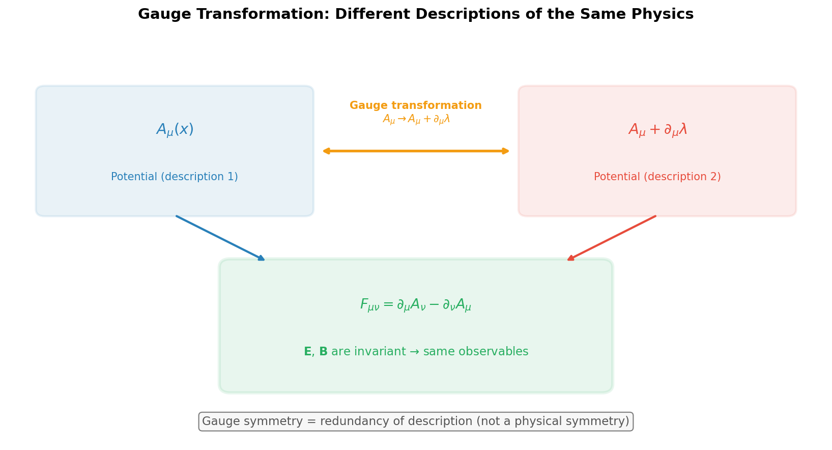
Fig. 6.1: Conceptual diagram of gauge transformation. A gauge transformation connects different descriptions of the same physics. The potential \(A_\mu\) changes, but the physical quantity \(F_{\mu\nu}\) (electric and magnetic fields) is invariant.
✅ Comprehension Check: Show that \(F_{\mu\nu}\) is invariant under the gauge transformation \(A_\mu \to A_\mu + \partial_\mu \lambda\) by substituting into definition (6.2).
Answer
\(F_{\mu\nu}' = \partial_\mu(A_\nu + \partial_\nu \lambda) - \partial_\nu(A_\mu + \partial_\mu \lambda) = \partial_\mu A_\nu - \partial_\nu A_\mu + \partial_\mu \partial_\nu \lambda - \partial_\nu \partial_\mu \lambda\). Since partial derivatives commute, \(\partial_\mu \partial_\nu \lambda = \partial_\nu \partial_\mu \lambda\). Therefore \(F_{\mu\nu}' = F_{\mu\nu}\).
🔵 Kai: But if there's redundancy, why do we bother using \(A_\mu\) at all? Wouldn't it be better to just use \(\mathbf{E}\) and \(\mathbf{B}\) from the start?
🟡 Lina: Actually, we can't write a nice Lagrangian using only \(\mathbf{E}\) and \(\mathbf{B}\). We need \(A_\mu\) to write a Lorentz-covariant Lagrangian. Moreover, in quantum mechanics, phenomena like the Aharonov-Bohm effect show that \(A_\mu\) itself plays a physical role. The Aharonov-Bohm effect is a remarkable phenomenon where the interference pattern of electrons passing through a region with \(\mathbf{B} = 0\) depends on the magnetic flux enclosed by that region (i.e., the line integral of \(\mathbf{A}\)). Even when \(\mathbf{E}\) and \(\mathbf{B}\) are zero, \(\mathbf{A}\) has physical effects—evidence that potentials are not merely computational tools. Even though it contains redundancy, there are deep reasons for using \(A_\mu\).
Gauge Symmetry and Local U(1) Transformations
🟡 Lina: Let's look at the gauge transformation (6.7) from the perspective of matter fields (fields of charged particles). The electromagnetic field \(A_\mu\) is the "force-carrying field," but we also need the receiving side—the field of particles carrying charge. To keep things simplest, let's use the complex scalar field from Ch. 4 as our representative "charged particle field." In Ch. 4 we wrote \(\hat{\psi}\) in the mode expansion, but here we'll write \(\phi\) to avoid confusion with the Dirac spinor. Its Lagrangian is
The complex scalar field has one component, so complex conjugate \(*\) and Hermitian conjugate \(\dagger\) mean the same thing. This Lagrangian is invariant under the global U(1) transformation
(\(\alpha\) is a constant). From Noether's theorem in Ch. 3, the conserved quantity corresponding to this symmetry was electric charge.
🔵 Kai: "Global" means rotating by the same \(\alpha\) everywhere in the universe, right?
🟡 Lina: Right. But now let's ask an ambitious question. Can we make the theory invariant even if we change the phase independently at each spacetime point? That is,
demanding invariance under this local transformation.
⚪ Mei: Since \(\alpha(x)\) depends on \(x\), extra terms will appear when we differentiate.
🟡 Lina: Exactly. \(\partial_\mu \phi \to e^{i\alpha(x)}(\partial_\mu \phi + i(\partial_\mu \alpha)\phi)\), and the extra \(i(\partial_\mu \alpha)\phi\) survives. The invariance of the Lagrangian is broken.
🔵 Kai: So local invariance is impossible?
🟡 Lina: No. This is where a brilliant idea comes in. The problem is that \(\partial_\mu(e^{i\alpha}\phi)\) produces an extra \(i(\partial_\mu \alpha)\phi\). To cancel this, we need "something" that compensates with \(-i(\partial_\mu \alpha)\) every time we differentiate.
Let's work backwards. We want \(D_\mu \phi\) to follow the same transformation rule as \(\phi\): \(D_\mu \phi \to e^{i\alpha} D_\mu \phi\). The ordinary derivative \(\partial_\mu\) alone produces the extra \(i(\partial_\mu \alpha)\phi\). So we add a "correction term" to the derivative such that, under the transformation, this correction produces exactly \(-i(\partial_\mu \alpha)\phi\) to cancel. The solution is to introduce a new field \(A_\mu\) and replace the ordinary derivative with a "covariant derivative":
Here \(q\) is a coupling constant that physically corresponds to the particle's charge (for the electron, \(q = -e\)). In the natural unit system of particle physics, in addition to \(c = \hbar = 1\), we also choose \(\varepsilon_0 = 1\) for electromagnetic units (this is called the Heaviside-Lorentz unit system). In SI units, the Coulomb force is \(F = q^2/(4\pi\varepsilon_0 r^2)\), so when \(\varepsilon_0\) disappears, \(q^2\) has dimensions of force × distance\(^2\). When \(\hbar = c = 1\) further unifies the dimensions of length, time, and energy, \(q^2/(4\pi)\) becomes dimensionless. Indeed, you can see this from the fact that the fine-structure constant \(\alpha = q^2/(4\pi) \approx 1/137\) is dimensionless. So in this unit system, the charge \(q\) itself is dimensionless.
🔵 Kai: Why \(+iq\)? Why not \(+q\) or \(+iA_\mu\)?
🟡 Lina: Good question. Working backwards makes it clear. Expanding \(\partial_\mu(e^{i\alpha}\phi)\) produces the extra term \(+i(\partial_\mu \alpha)\phi\). To cancel this, we need a term in \(D_\mu\) that generates \(-i(\partial_\mu \alpha)\phi\). If \(A_\mu\) shifts by \(\Delta A_\mu\) under the transformation, the contribution from the correction term \(iq A_\mu\) in \(D_\mu\) is \(iq \cdot \Delta A_\mu \cdot \phi\). For this to equal \(-i(\partial_\mu \alpha)\phi\), we need \(iq \cdot \Delta A_\mu = -i(\partial_\mu \alpha)\), i.e., \(\Delta A_\mu = -\frac{1}{q}\partial_\mu \alpha\). Conversely, unless the coefficient in \(D_\mu\) is \(iq\) (the product of \(i\) and \(q\)), this cancellation won't work.
⚪ Mei: So the \(i\) comes from the phase transformation \(e^{i\alpha}\), and \(q\) is the coupling constant Lina mentioned—the magnitude of the charge.
🟡 Lina: Right. The relationship between the gauge function \(\lambda\) in equation (6.7) and the matter field phase \(\alpha\) is \(\lambda = -\alpha/q\). Substituting into equation (6.7) gives
The minus sign appears because, to cancel the extra term \(+i(\partial_\mu \alpha)\phi\) in the transformation of \(D_\mu \phi\), \(A_\mu\) needs to shift by \(-\frac{1}{q}\partial_\mu \alpha\). Under this correspondence, \(D_\mu \phi\) transforms with the same rule as \(\phi\):
🔵 Kai: Wait a moment. Why does that work? I'd like to verify it by calculation.
🟡 Lina: Good. Let's do it. We compute the transformed \(D_\mu' \phi'\):
Expanding \(\partial_\mu(e^{i\alpha}\phi)\) using the product rule:
The first and fourth terms cancel:
⚪ Mei: I see. The transformation of \(A_\mu\) absorbs exactly the extra \(\partial_\mu \alpha\) term. If \(D_\mu \phi\) follows the same transformation rule as \(\phi\), then the kinetic term of the Lagrangian should automatically be gauge invariant.
🟡 Lina: Exactly. If we replace the kinetic term \(\partial_\mu\phi^*\,\partial^\mu\phi\) with \((D^\mu \phi)^\dagger (D_\mu \phi)\), then from \(D_\mu\phi \to e^{i\alpha}D_\mu\phi\) and \((D_\mu\phi)^\dagger \to (D_\mu\phi)^\dagger e^{-i\alpha}\), the phases cancel and it's automatically gauge invariant.
🟡 Lina: Yes. And if we add the gauge-invariant \(-\frac{1}{4}F_{\mu\nu}F^{\mu\nu}\) as the Lagrangian for \(A_\mu\) itself, the entire theory becomes gauge invariant.
Here a remarkable message emerges:
Simply demanding local U(1) symmetry uniquely determines both the existence of the electromagnetic field \(A_\mu\) and the form of its coupling to matter fields. Symmetry gives birth to force.
🔵 Kai: Amazing... So the answer to "why does electromagnetic force exist?" is "because we allow local phase freedom"?
🟡 Lina: Exactly. And this principle isn't limited to electromagnetism. Local SU(2)×U(1) symmetry leads to the weak force, and local SU(3) symmetry leads to the strong force. We'll study this in detail in Ch. 17 on Yang-Mills theory.
✅ Comprehension Check: Under what symmetry requirement does the need arise to replace ordinary derivatives \(\partial_\mu\) with covariant derivatives \(D_\mu = \partial_\mu + iqA_\mu\)? And what is consequently derived?
Answer
When demanding local U(1) symmetry (invariance of the Lagrangian under independent phase changes at each spacetime point). The ordinary derivative produces an extra \(\partial_\mu \alpha\) term in \(\partial_\mu(e^{i\alpha(x)}\psi)\), so a new field \(A_\mu\) must be introduced to absorb it via the covariant derivative. As a result, the existence of the electromagnetic field and the form of its coupling to matter fields are uniquely determined.
6.3 Gauge Symmetry Obstructs Quantization—The Vanishing Conjugate Momentum
🟡 Lina: Having confirmed the beauty of gauge symmetry, we now face the difficulty head-on. Let's try to canonically quantize the electromagnetic field.
What was the first step when we quantized the scalar field in Ch. 4?
🔵 Kai: Um... defining the conjugate momentum for the field and imposing commutation relations, right?
🟡 Lina: Right. We defined the conjugate momentum \(\pi = \partial \mathcal{L}/\partial \dot{\phi}\) and imposed the equal-time commutation relation \([\phi(\mathbf{x},t),\, \pi(\mathbf{y},t)] = i\delta^3(\mathbf{x} - \mathbf{y})\). Now let's try the same thing for \(A_\mu\). The conjugate momentum of \(A_\mu\) is
Expanding the Lagrangian \(\mathcal{L} = -\frac{1}{4}F_{\mu\nu}F^{\mu\nu}\) and differentiating with respect to \(\partial_0 A_\mu\), for the spatial components \(\mu = i\) we get
(Let me verify the calculation. For \(\mathcal{L} = -\frac{1}{4}F_{\mu\nu}F^{\mu\nu}\), we have \(\frac{\partial \mathcal{L}}{\partial(\partial_\rho A_\sigma)} = -F^{\rho\sigma}\) (the \(-1/4\) coefficient and the factor of 2×2 from antisymmetry cancel). Taking \(\rho = 0\), \(\sigma = i\) gives \(\pi^i = -F^{0i}\). As we confirmed in equation (6.4), \(F^{0i} = -E^i\), so \(\pi^i = -(-E^i) = E^i\). In other words, the conjugate momentum of \(\mathbf{A}\) is the electric field \(\mathbf{E}\).) So far so good. The problem is the time component \(\mu = 0\):
🔵 Kai: Zero!? Why?
🟡 Lina: Look at the definition of \(F_{\mu\nu}\). \(F_{00} = \partial_0 A_0 - \partial_0 A_0 = 0\) (from antisymmetry). And \(F_{0i} = \partial_0 A_i - \partial_i A_0\) does not contain \(\partial_0 A_0\). In other words, \(\dot{A}_0 = \partial_0 A_0\) never appears in the Lagrangian.
⚪ Mei: If \(\dot{A}_0\) appears nowhere, then the term corresponding to \(A_0\)'s "velocity" is zero... For the scalar field, \(\dot{\phi}\) created the kinetic energy.
🟡 Lina: Right. Since \(A_0\) has no term corresponding to kinetic energy, it cannot be treated as an independent dynamical variable. \(\pi^0 = 0\) means the canonical commutation relation
cannot be written. The left side is \([A_0, 0] = 0\) but the right side is \(i\delta^3(\mathbf{x} - \mathbf{y}) \neq 0\). A contradiction arises.
🔵 Kai: Whoa... This problem never came up with the scalar field or Dirac field.
🟡 Lina: Right. This is a problem unique to gauge symmetry. Physically, it reflects the fact that not all 4 components of \(A_\mu\) are independent physical degrees of freedom. The fact that physics doesn't change under \(A_\mu \to A_\mu + \partial_\mu \lambda\) means that among the configurations of \(A_\mu\), "real physics" and "redundant description" are mixed together.
🔵 Kai: Then how many of the 4 components are truly physical degrees of freedom?
🟡 Lina: First, since \(A_0\) is not a dynamical variable, 4 → 3. Then the gauge transformation freedom \(\lambda(x)\) removes one more: 3 → 2. The physical degrees of freedom are 2. This corresponds to the fact that light has 2 polarizations (e.g., horizontal and vertical).
🔵 Kai: A 4-component field with only 2 physical degrees of freedom... The other 2 are gauge redundancy.
🟡 Lina: Right. We can't proceed with quantization without handling this redundancy. The procedure for handling it is called gauge fixing. I've illustrated this reduction of degrees of freedom in Fig. 6.2 "Counting the physical degrees of freedom of the electromagnetic field".
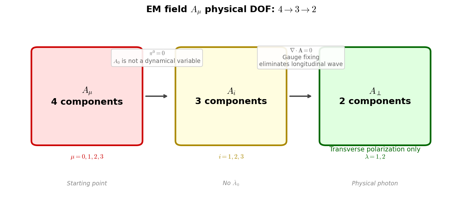
Fig. 6.2: Counting the physical degrees of freedom of the electromagnetic field. From the 4 components of \(A_\mu\), one is removed by \(\pi^0 = 0\) (\(A_0\) is not a dynamical variable), and one more by the gauge-fixing condition, leaving only the 2 transverse polarizations of the photon as physical degrees of freedom.
✅ Comprehension Check: The electromagnetic field \(A_\mu\) has 4 components, but only 2 physical degrees of freedom. Explain why the number reduces from 4 to 2.
Answer
First, \(A_0\) is not an independent dynamical variable because the Lagrangian contains no \(\dot{A}_0\), reducing 4 → 3. Furthermore, there is one degree of gauge transformation freedom \(A_\mu \to A_\mu + \partial_\mu \lambda\), and by choosing the arbitrary function \(\lambda(x)\) we can fix one component, reducing 3 → 2. The remaining 2 degrees of freedom correspond to the 2 transverse polarizations of the photon.
✅ Comprehension Check: Explain from the definition of \(F_{\mu\nu}\) why the Maxwell field Lagrangian \(\mathcal{L} = -\frac{1}{4}F_{\mu\nu}F^{\mu\nu}\) contains no \(\dot{A}_0\).
Answer
In \(F_{\mu\nu} = \partial_\mu A_\nu - \partial_\nu A_\mu\), the only terms that could contain \(\partial_0 A_0\) are those of the form \(F_{0\nu}\), but \(F_{00} = \partial_0 A_0 - \partial_0 A_0 = 0\), and \(F_{0i} = \partial_0 A_i - \partial_i A_0\) contains \(\partial_0 A_i\) but not \(\partial_0 A_0\). Therefore \(F_{\mu\nu}F^{\mu\nu}\) also contains no \(\dot{A}_0\), and \(\pi^0 = \partial\mathcal{L}/\partial\dot{A}_0 = 0\).
6.4 Quantization in Coulomb Gauge—Where Physical Degrees of Freedom Are Visible
🟡 Lina: As our first approach to gauge fixing, let me introduce the Coulomb gauge. The condition is
That is, the divergence of the vector potential \(\mathbf{A}\) is zero.
🔵 Kai: Why choose this condition?
🟡 Lina: There are two advantages. First, \(\nabla \cdot \mathbf{A} = 0\) means \(\mathbf{A}\) is transverse. In Fourier space, \(\mathbf{k} \cdot \tilde{\mathbf{A}}(\mathbf{k}) = 0\), meaning \(\mathbf{A}\) has only components perpendicular to the wave's propagation direction \(\mathbf{k}\). The physical polarizations are directly visible.
⚪ Mei: Intuitively, the strategy is to "drop the longitudinal part from the start."
🟡 Lina: Second, in vacuum we can set \(A_0 = 0\). From equation (6.3), \(\nabla \cdot \mathbf{E} = -\nabla^2 A_0 - \partial_t(\nabla \cdot \mathbf{A})\), but under the Coulomb gauge \(\nabla \cdot \mathbf{A} = 0\) the second term vanishes, so Gauss's law \(\nabla \cdot \mathbf{E} = 0\) becomes \(\nabla^2 A_0 = 0\). Imposing boundary conditions (\(A_0 \to 0\) at infinity), the only solution is \(A_0 = 0\). This is a consequence of the uniqueness theorem for the Laplace equation. Intuitively, a function satisfying \(\nabla^2 A_0 = 0\) (called a harmonic function) has the property that "the value at any point equals the average of its surroundings." If \(A_0\) were positive somewhere, its surrounding average would also have to be positive, and the surroundings of those, and so on—the positive value would propagate to infinity. This contradicts the boundary condition \(A_0 \to 0\) (vanishing at infinity). Therefore \(A_0 \equiv 0\) is the only possibility.
🔵 Kai: I see, so \(A_0\) vanishing isn't just a "choice" but necessarily follows from the equation and boundary conditions.
⚪ Mei: So in Coulomb gauge, \(A_0\) vanishes, and furthermore the gauge condition \(\nabla \cdot \mathbf{A} = 0\) eliminates the longitudinal component of \(\mathbf{A}\). The remaining dynamical variables are just the 2 transverse components.
🟡 Lina: Perfect summary. Now let's proceed with the quantization concretely.
Fourier Expansion and Polarization Vectors
🟡 Lina: Let's write the equation of motion (6.5) \(\partial_\mu F^{\mu\nu} = 0\) in Coulomb gauge (\(\nabla \cdot \mathbf{A} = 0\), \(A_0 = 0\)). The goal is to show that "each component of \(\mathbf{A}\) satisfies the wave equation \(\Box A^i = 0\)"—the mathematical expression of light propagating as a wave. Taking the \(\nu = i\) component:
In Coulomb gauge with \(A_0 = 0\), from equation (6.3) we have \(E^i = -\dot{A}^i\). As confirmed in equation (6.4), \(F^{0i} = -E^i\), so \(F^{0i} = -(-\dot{A}^i) = \dot{A}^i\).
🔵 Kai: So \(\partial_0 F^{0i} = \ddot{A}^i\).
🟡 Lina: Right. Next let's compute \(\partial_j F^{ji}\). \(F^{ji} = \eta^{j\alpha}\eta^{i\beta}F_{\alpha\beta}\), but with the diagonal metric, \(\eta^{j\alpha}\) is nonzero only for \(\alpha = j\), and similarly \(\eta^{i\beta}\) is nonzero only for \(\beta = i\). So in the sum over \(\alpha\), \(\beta\), only the \(\alpha = j\), \(\beta = i\) term survives: \(F^{ji} = \eta^{j\alpha}\eta^{i\beta}F_{\alpha\beta}\big|_{\alpha=j,\,\beta=i} = \eta^{jj}\eta^{ii}F_{ji}\) (\(j\), \(i\) are fixed free indices with no summation. Since the metric is diagonal, terms with \(\alpha \neq j\) or \(\beta \neq i\) vanish) \(= (-1)(-1)F_{ji} = F_{ji} = \partial_j A_i - \partial_i A_j\). Here, since \(\partial^j = \eta^{jk}\partial_k = -\partial_j\) and \(A^i = -A_i\), we have \(\partial^j A^i = (-\partial_j)(-A_i) = \partial_j A_i\). Therefore, writing in raised-index form also gives \(F^{ji} = \partial^j A^i - \partial^i A^j\) with the same value. Using this:
Now recall the index-raising operation. As we learned in Ch. 2, with the QFT metric \(\eta^{jk} = -\delta^{jk}\) (spatial components), we have \(\partial^j = \eta^{jk}\partial_k = -\partial_j\). Therefore \(\partial_j \partial^j\) (summing over \(j\)) \(= \sum_{j=1}^3 \partial_j \partial^j = \sum_{j=1}^3 \partial_j(-\partial_j) = -(\partial_1^2 + \partial_2^2 + \partial_3^2) = -\nabla^2\).
🔵 Kai: The minus in the metric makes \(\partial_j \partial^j = -\nabla^2\).
🟡 Lina: Right. The second term is \(-\partial^i(\partial_j A^j)\), so let me clarify the relationship between the physical divergence \(\nabla \cdot \mathbf{A}\) and the index contraction \(\partial_j A^j\). The physical divergence of the vector potential is \(\nabla \cdot \mathbf{A} = \sum_j \frac{\partial A^j}{\partial x^j} = \sum_j \partial_j A^j\) (\(A^j\) are contravariant components). The Coulomb gauge condition \(\nabla \cdot \mathbf{A} = 0\) directly means \(\partial_j A^j = 0\). Therefore the second term \(-\partial^i(\partial_j A^j) = 0\) vanishes, giving \(\partial_j F^{ji} = -\nabla^2 A^i\).
Combining the two: \(\ddot{A}^i - \nabla^2 A^i = 0\), namely
Each component satisfies the wave equation. Let's expand the solution in plane waves:
Here \(\omega_{\mathbf{k}} = |\mathbf{k}|\) (since the photon is massless, \(\omega = |\mathbf{k}|c\), and in natural units \(c = 1\) gives \(\omega = |\mathbf{k}|\)), \(kx = \omega_{\mathbf{k}} t - \mathbf{k} \cdot \mathbf{x}\).
\(\boldsymbol{\epsilon}(\mathbf{k}, \lambda)\) is the polarization vector, with \(\lambda = 1, 2\).
🔵 Kai: What's a polarization vector?
🟡 Lina: It's a vector representing the oscillation direction of light. Writing the Coulomb gauge condition \(\nabla \cdot \mathbf{A} = 0\) in Fourier space gives
This means the polarization vector must be perpendicular to the wave vector \(\mathbf{k}\) (the propagation direction). In 3-dimensional space, the plane perpendicular to \(\mathbf{k}\) is 2-dimensional, so there are \(\lambda = 1, 2\) independent polarization vectors.
⚪ Mei: The perpendicular plane is 2-dimensional, so there are 2 basis vectors. That corresponds to the number of physical polarizations.
🟡 Lina: Right. For example, if \(\mathbf{k}\) points in the \(z\) direction:
These form the linear polarization basis. For circular polarization:
These correspond to helicity \(\pm 1\) states.
🔵 Kai: What's "helicity"?
🟡 Lina: It's a quantity that tells you whether the spin (like rotation) is right-handed or left-handed around the particle's direction of motion. More precisely, it's the component of spin angular momentum along the direction of propagation. The photon is a spin-1 particle, but because it's massless, its helicity can only be \(+1\) (right circular polarization) or \(-1\) (left circular polarization). The \(0\) (longitudinal polarization) doesn't exist for massless particles.
🔵 Kai: Why can't a massless particle have helicity \(0\)? If it's spin 1, shouldn't there be three values: \(-1, 0, +1\)?
🟡 Lina: Good question. For a massive particle, there would indeed be 3. But a massless particle travels at the speed of light, so no "rest frame" exists. Without a rest frame, only rotations in the plane perpendicular to the direction of motion (transverse polarization) can be physically defined. Intuitively, since you can't "overtake and look from the front" at a particle traveling at light speed, there's no way to physically distinguish oscillations along the direction of motion (longitudinal polarization). And mathematically, the state corresponding to longitudinal polarization with helicity \(0\) can be eliminated by a gauge transformation—it's part of the gauge symmetry redundancy. This is a consequence of gauge symmetry.
⚪ Mei: "Can't overtake it, so can't distinguish longitudinal oscillation"—the physical intuition and the mathematical gauge symmetry story are connected.
Canonical Commutation Relations
🟡 Lina: Now for the quantization step. As we saw in equation (6.16), the conjugate momentum for \(A_i\) is \(\pi^i = -F^{0i} = E^i\). In Coulomb gauge with \(A_0 = 0\), equation (6.3) simplifies from \(\mathbf{E} = -\nabla A_0 - \dot{\mathbf{A}}\) to \(\mathbf{E} = -\dot{\mathbf{A}}\). So in Coulomb gauge \(E^i = -\dot{A}^i\), and combined with equation (6.16) \(\pi^i = E^i\), we get \(\pi^i = -\dot{A}^i\). (Let me organize the upper/lower indices. From equation (6.16), \(\pi^i = E^i\) (upper). To lower the spatial index, use \(\eta_{ji} = -\delta_{ji}\): \(\pi_j = \eta_{ji}\pi^i = -\pi^j = -E^j\). Similarly \(A_i = \eta_{ij}A^j = -A^j\), so \(\dot{A}_i = -\dot{A}^i\). In Coulomb gauge, \(E^i = -\dot{A}^i\), so \(\pi^i = E^i = -\dot{A}^i = \dot{A}_i\), which is consistent. In equation (6.24), we use the lowered-index form \([A_i, \pi_j]\) because it makes the correspondence with the transverse projection operator \(\delta_{ij}^\perp\) clearer.)
We impose canonical commutation relations. However, a caution is needed here. Equation (6.20) writes \(\mathbf{A}\) in contravariant components \(A^i\), but in the canonical formalism it's standard to use covariant components \(A_i = -A^i\) (as previewed at the beginning). If we naively write \([A_i(\mathbf{x}, t),\, \pi_j(\mathbf{y}, t)] = i\delta_{ij}\,\delta^3(\mathbf{x} - \mathbf{y})\), the right side includes all components of \(A_i\) (both longitudinal and transverse). But in Coulomb gauge with \(\nabla \cdot \mathbf{A} = 0\), \(A_i\) has no longitudinal component. Writing a commutation relation for a nonexistent component is contradictory. So we need to include a projection onto "transverse components only" on the right side:
where
🔵 Kai: Instead of the ordinary \(\delta_{ij}\,\delta^3(\mathbf{x}-\mathbf{y})\), you're subtracting \(k_i k_j/|\mathbf{k}|^2\).
🟡 Lina: Right. \(\delta_{ij} - k_i k_j/|\mathbf{k}|^2\) is the projection operator that "removes the component along \(\mathbf{k}\)." Specifically, multiplying any vector \(v_j\) by this gives \(v_i - k_i(\mathbf{k}\cdot\mathbf{v})/|\mathbf{k}|^2\), cleanly subtracting the \(\mathbf{k}\)-direction component. This excludes the longitudinal component from the commutation relation to be consistent with the constraint \(\nabla \cdot \mathbf{A} = 0\) (i.e., \(\mathbf{k} \cdot \tilde{\mathbf{A}} = 0\) in Fourier space).
Translated into the language of creation and annihilation operators:
⚪ Mei: The same form of commutation relations as for the scalar field. But with a polarization index \(\lambda\) added. If it has the same structure as the previous chapter, then \(a^\dagger(\mathbf{k}, \lambda)\) is the operator that "creates one photon with momentum \(\mathbf{k}\) and polarization \(\lambda\)."
🟡 Lina: Right. The Hamiltonian (energy operator) can also be computed:
(zero-point energy removed by normal ordering). This represents "each mode \((\mathbf{k}, \lambda)\) photon carries energy \(\omega_{\mathbf{k}} = |\mathbf{k}|\)."
🔵 Kai: Planck's \(E = \hbar\omega\) emerges naturally! (In natural units \(\hbar = 1\), so \(E = \omega\).) So the quantization that Planck introduced as a "hypothesis" in 1900 comes out automatically when you quantize the field. But wait—you casually said "removed by normal ordering," but each mode has zero-point energy \(\frac{1}{2}\omega\), and there are infinitely many modes, so the total is infinite. It sounds like you're throwing away infinity...
⚪ Mei: Right, the same problem came up in Ch. 4 with the scalar field.
🟡 Lina: Good question. The zero-point energy problem is actually a deep topic that we also touched on in Ch. 4 for the scalar field. Normal ordering is an operation that "shifts the energy reference point," and it's justified as long as only relative energy differences are physically meaningful. However, when gravity is considered, it connects to the unsolved cosmological constant problem. For now, accept it as "a prescription for setting the energy reference of the free field."
🔵 Kai: I see... So only "energy differences" are physical. But wait—gravity responds to the absolute value of energy, right? Then doesn't the infinity we "discarded" by normal ordering come back as soon as we consider gravity?
🟡 Lina: Exactly. That's the heart of the cosmological constant problem. There's a discrepancy of a factor of \(10^{120}\) between the vacuum energy of quantum field theory and cosmological observations—one of the greatest unsolved problems in modern physics. But let's focus on free field quantization for now.
🔵 Kai: Understood. I'll keep it in the back of my mind as an unsolved problem.
🟡 Lina: Please do. Now, let's confirm something important. The quantum of light—the photon—has been born from field quantization.
✅ Comprehension Check: In the quantization of the electromagnetic field in Coulomb gauge, what does the state created by the creation operator \(a^\dagger(\mathbf{k}, \lambda)\) physically represent?
Answer
It represents the state of one photon with momentum \(\mathbf{k}\) and polarization \(\lambda\) (\(\lambda = 1\) or \(2\)) added to the vacuum. From the Hamiltonian (6.28), this photon has energy \(\omega_{\mathbf{k}} = |\mathbf{k}|\), corresponding to Planck's relation \(E = \hbar\omega\) (\(E = \omega\) in natural units).
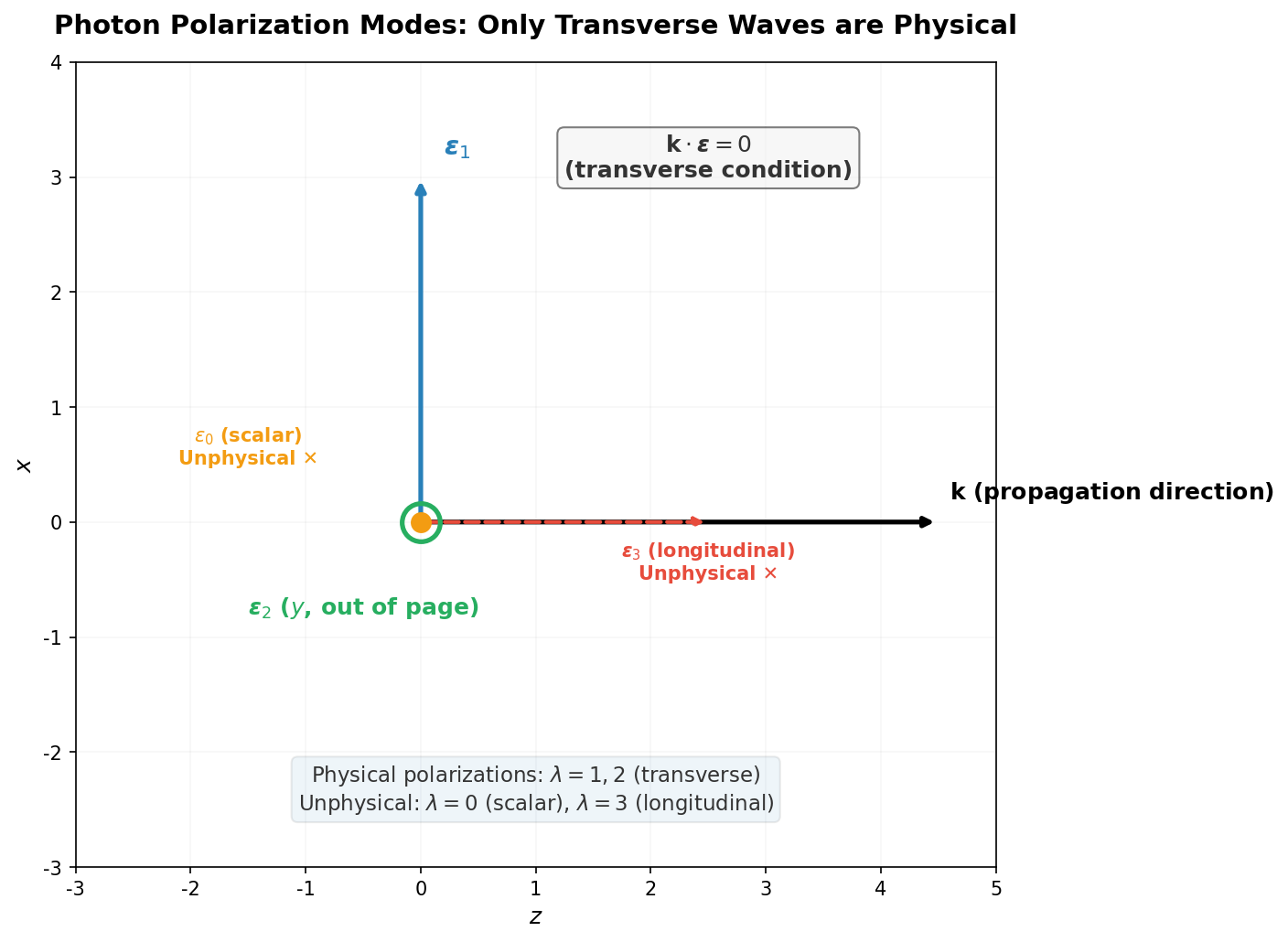
Fig. 6.3: Photon polarization modes. The transverse condition \(\mathbf{k} \cdot \boldsymbol{\epsilon} = 0\) allows only 2 physical polarizations (\(\lambda = 1, 2\)) perpendicular to the propagation direction. In the Lorenz gauge discussed later (6.6 "Quantization in Lorenz Gauge—Covariant but Ghosts Appear"), longitudinal and scalar polarizations are formally introduced, but these are unphysical and ultimately eliminated.
Fig. 6.3 "Photon polarization modes" summarizes the photon polarization modes.
✅ Comprehension Check: Explain why there are 2 physical polarizations for photons in Coulomb gauge, from the condition \(\mathbf{k} \cdot \boldsymbol{\epsilon} = 0\).
Answer
\(\boldsymbol{\epsilon}\) is a 3-dimensional vector, but the condition \(\mathbf{k} \cdot \boldsymbol{\epsilon} = 0\) forbids the component along \(\mathbf{k}\). The plane perpendicular to \(\mathbf{k}\) is 2-dimensional, so there are 2 independent polarization vectors. These correspond to the 2 physical polarizations of the photon.
📝 Exercises:
- Realizability of Coulomb gauge → Problem M-2. Counting Degrees of Freedom in Coulomb Gauge
6.5 Problems with Coulomb Gauge
🟡 Lina: Coulomb gauge has the great advantage that physical degrees of freedom are explicitly visible. But it also has a serious drawback.
🔵 Kai: What is it?
🟡 Lina: Lorentz covariance is not manifest. The condition \(\nabla \cdot \mathbf{A} = 0\) involves only spatial derivatives and doesn't treat time and space on equal footing. That is, even if \(\nabla \cdot \mathbf{A} = 0\) holds in one inertial frame, boosting to another frame generally breaks this condition.
⚪ Mei: Meaning the consistency with special relativity is hard to see. It's difficult to verify whether Lorentz invariance is maintained during calculations.
🟡 Lina: Exactly. For actual scattering amplitude calculations, a Lorentz-covariant formalism is overwhelmingly more convenient. That's where the Lorenz gauge comes in.
Terminology note: The "Lorenz" in Lorenz gauge refers to Ludvig Lorenz, a Danish physicist, who is different from Hendrik Lorentz of the Lorentz transformation. It's confusing, but that's how it is historically.
✅ Comprehension Check: What does it mean that the Coulomb gauge condition \(\nabla \cdot \mathbf{A} = 0\) is not Lorentz covariant?
Answer
\(\nabla \cdot \mathbf{A} = 0\) involves only spatial derivatives and doesn't treat time and space on equal footing. Therefore, even if this condition holds in one inertial frame, a Lorentz boost to another frame generally breaks it. The drawback is that it's difficult to verify whether Lorentz invariance is maintained during calculations.
6.6 Quantization in Lorenz Gauge—Covariant but Ghosts Appear
Lorenz Gauge Condition
🟡 Lina: The Lorenz gauge condition is
Since this is written in four-vector form, it's Lorentz covariant. If this condition holds in one inertial frame, it holds in all inertial frames.
🔵 Kai: Compared to the Coulomb gauge \(\nabla \cdot \mathbf{A} = 0\), this also includes the time component \(\partial_0 A^0\).
🟡 Lina: Right. \(\partial_\mu A^\mu = \partial_0 A^0 + \nabla \cdot \mathbf{A} = 0\), treating time and space on equal footing.
Under the Lorenz gauge, the equation of motion (6.5) takes a simple form. Writing equation (6.5) in terms of \(A_\nu\):
Using the Lorenz gauge condition \(\partial_\mu A^\mu = 0\), the second term vanishes:
Each component independently satisfies the wave equation! Very simple.
⚪ Mei: In Coulomb gauge, dealing with index raising/lowering and the Laplacian was complicated, but in Lorenz gauge we get \(\Box A^\nu = 0\) immediately—that's certainly convenient.
Adding a Gauge-Fixing Term
🟡 Lina: However, performing canonical quantization in Lorenz gauge requires some ingenuity. With the original Lagrangian (6.1) alone, the \(\pi^0 = 0\) problem persists. So we add a gauge-fixing term to the Lagrangian.
The idea is this: instead of imposing the Lorenz gauge condition \(\partial_\mu A^\mu = 0\) "hard," we add a term that gives an "energy penalty" to configurations with \(\partial_\mu A^\mu \neq 0\). Just as a spring potential \(\frac{1}{2}kx^2\) penalizes deviations from \(x = 0\), the term \((\partial_\mu A^\mu)^2\) penalizes deviations from the Lorenz condition:
Here \(\xi\) is an arbitrary parameter (the gauge parameter) controlling the "strength" of the penalty. The choice \(\xi = 1\) is called the Feynman gauge.
🔵 Kai: Doesn't adding the gauge-fixing term break gauge symmetry?
🟡 Lina: Sharp question. Indeed, \((\partial_\mu A^\mu)^2\) is not invariant under gauge transformation (6.7). So gauge symmetry is explicitly broken. However, the final physical observables (scattering cross sections, etc.) can be shown to be independent of \(\xi\). This is a very deep result—the "afterglow" of gauge symmetry protects the physical results.
⚪ Mei: So during the calculation we fix the gauge and break the symmetry, but the final result doesn't depend on the choice of gauge.
✅ Comprehension Check: What is the purpose of adding the gauge-fixing term \(-\frac{1}{2\xi}(\partial_\mu A^\mu)^2\) to the Lagrangian? And why is it not problematic despite breaking gauge symmetry?
Answer
The purpose is to resolve the problem that with the original Lagrangian, \(\pi^0 = 0\) prevents canonical quantization. The gauge-fixing term adds terms containing \(\dot{A}_0\), making \(\pi^0 \neq 0\). Although gauge symmetry is explicitly broken, the final physical observables (scattering amplitudes, etc.) can be shown to be independent of the gauge parameter \(\xi\), so physical conclusions are unaffected.
🟡 Lina: Exactly. Now let's see what changes by adding the gauge-fixing term. Computing the conjugate momentum for \(A^0\) (as we saw in equation (6.17), the contribution from \(-\frac{1}{4}F_{\mu\nu}F^{\mu\nu}\) is zero, so only the gauge-fixing term contributes):
🔵 Kai: It's no longer zero! The gauge-fixing term "revived" \(\dot{A}_0\).
🟡 Lina: Let me verify the calculation. \(\partial_\mu A^\mu = \partial_0 A^0 + \partial_1 A^1 + \partial_2 A^2 + \partial_3 A^3\), which contains \(\dot{A}_0 \equiv \partial_0 A_0 = \partial A_0/\partial t\) (index raising/lowering uses \(A^\mu = \eta^{\mu\nu}A_\nu\) (summing over \(\nu\)), but with diagonal metric \(A^0 = \eta^{0\nu}A_\nu = \eta^{00}A_0 = (+1)A_0 = A_0\). The time component doesn't change sign between upper and lower. So \(\partial_0 A_0 = \partial_0 A^0\). However, spatial components have \(A^i = \eta^{i\nu}A_\nu\) (sum over \(\nu\)) \(= \eta^{ii}A_i\) (only \(\nu = i\) term is nonzero for diagonal metric) \(= (-1)A_i = -A_i\), so the sign changes—be careful). The gauge-fixing term \(-\frac{1}{2\xi}(\partial_\mu A^\mu)^2\) differentiated with respect to \(\partial_0 A_0\), using the chain rule:
(Here, among \(\partial_\mu A^\mu = \partial_0 A^0 + \partial_1 A^1 + \partial_2 A^2 + \partial_3 A^3\), the only term containing \(\partial_0 A_0\) is the first term \(\partial_0 A^0 = \partial_0 A_0\) (since \(A^0 = A_0\)). The remaining \(\partial_i A^i\) are spatial derivatives independent of \(\partial_0 A_0\). Therefore \(\partial(\partial_\mu A^\mu)/\partial(\partial_0 A_0) = 1\).)
Because the gauge-fixing term added a term containing \(\dot{A}_0\) to the Lagrangian, \(\pi^0\) is no longer identically zero. Solving inversely gives \(\dot{A}_0 = -\xi\pi^0 - \partial_i A^i\), so \(A_0\) and \(\pi^0\) can be treated as an independent pair of canonical variables. Now canonical commutation relations can be written for all 4 components:
⚪ Mei: Now it fits the same "template" as the scalar field. All 4 components can be quantized on equal footing.
Four Polarizations and Fourier Expansion
🟡 Lina: Let's derive the equation of motion in Feynman gauge (\(\xi = 1\)). We apply the Euler-Lagrange equation to the Lagrangian \(\mathcal{L}_{\text{gf}} = -\frac{1}{4}F_{\mu\nu}F^{\mu\nu} - \frac{1}{2}(\partial_\mu A^\mu)^2\) from equation (6.31). Since \(\mathcal{L}_{\text{gf}}\) doesn't contain \(A_\sigma\) itself, the second term of the Euler-Lagrange equation \(\partial_\rho \frac{\partial \mathcal{L}}{\partial(\partial_\rho A_\sigma)} - \frac{\partial \mathcal{L}}{\partial A_\sigma} = 0\) is zero. Let's compute the first term by splitting it into two parts.
First, the contribution from \(-\frac{1}{4}F_{\mu\nu}F^{\mu\nu}\). As in the derivation of equation (6.5), \(\frac{\partial(-\frac{1}{4}F_{\mu\nu}F^{\mu\nu})}{\partial(\partial_\rho A_\sigma)} = -F^{\rho\sigma}\), and applying \(\partial_\rho\) gives \(-\partial_\rho F^{\rho\sigma}\). Substituting \(F^{\rho\sigma} = \partial^\rho A^\sigma - \partial^\sigma A^\rho\) gives \(\partial_\rho F^{\rho\sigma} = \partial_\rho(\partial^\rho A^\sigma - \partial^\sigma A^\rho) = \Box A^\sigma - \partial^\sigma(\partial_\rho A^\rho)\), so it can be written as \(-(\Box A^\sigma - \partial^\sigma(\partial_\mu A^\mu))\).
🔵 Kai: Next is the gauge-fixing term.
🟡 Lina: Right. Let's compute the contribution from \(-\frac{1}{2}(\partial_\mu A^\mu)^2\). Writing \(\partial_\mu A^\mu = \eta^{\alpha\beta}\partial_\alpha A_\beta\), we get \(\frac{\partial}{\partial(\partial_\rho A_\sigma)}(\eta^{\alpha\beta}\partial_\alpha A_\beta) = \eta^{\alpha\beta}\delta^\rho_\alpha\delta^\sigma_\beta = \eta^{\rho\sigma}\), so
Applying \(\partial_\rho\) gives \(-\partial^\sigma(\partial_\mu A^\mu)\).
🔵 Kai: Now we have both contributions. What happens when we add them?
🟡 Lina: Let's add them together. Relabeling index \(\sigma\) to \(\nu\) and combining:
The \(\partial^\nu(\partial_\mu A^\mu)\) terms cancel:
🔵 Kai: Oh, they cancel beautifully! In Feynman gauge the two terms exactly cancel each other.
🟡 Lina: Each component independently satisfies the massless Klein-Gordon equation, so the expansion is
Here 4 polarization vectors \(\epsilon^\mu(\mathbf{k}, \lambda)\) with \(\lambda = 0, 1, 2, 3\) appear.
🔵 Kai: Four? But you said earlier that there are only 2 physical degrees of freedom...
🟡 Lina: Good observation. In Lorenz gauge, to maintain Lorentz covariance, we quantize all 4 components of \(A_\mu\) on equal footing. Since \(A_\mu\) is a 4-component vector, the "oscillation direction" of each Fourier mode must also be specified in 4-dimensional space—just as a 3-dimensional wave needs 3 basis vectors for oscillation directions, in 4 dimensions we need 4 bases (polarization vectors). The Lorenz gauge condition \(\partial_\mu A^\mu = 0\) is imposed not as an operator identity but as a condition on physical states (the Gupta-Bleuler condition) later. So at the expansion stage all 4 polarizations are needed, and unphysical components are "removed" afterward using a prescription.
Let's look at the 4 polarizations concretely. For \(\mathbf{k} = (0, 0, k)\) (the \(z\) direction):
Table 6.2: Classification of the 4 polarization vectors of the photon (for \(\mathbf{k} = (0,0,k)\))
| \(\lambda\) | Name | \(\epsilon^\mu(\mathbf{k}, \lambda)\) | Nature |
|---|---|---|---|
| 1 | Transverse | \((0, 1, 0, 0)\) | Physical |
| 2 | Transverse | \((0, 0, 1, 0)\) | Physical |
| 3 | Longitudinal | \((0, 0, 0, 1)\) | Unphysical |
| 0 | Scalar | \((1, 0, 0, 0)\) | Unphysical |
⚪ Mei: \(\lambda = 1, 2\) are physical light polarizations, while \(\lambda = 3\) (propagation direction) and \(\lambda = 0\) (time direction) are unphysical. In Coulomb gauge these were excluded from the start, but here we temporarily keep everything.
🟡 Lina: One note: this table shows a simplified form with \(\mathbf{k}\) along the \(z\)-axis. The transverse polarizations (\(\lambda = 1, 2\)) satisfy \(k_\mu \epsilon^\mu(\mathbf{k}, \lambda) = 0\), but the scalar polarization (\(\lambda = 0\)) and longitudinal polarization (\(\lambda = 3\)) individually do not (in 6.7 "The Gupta-Bleuler Method—Confining the Ghosts" we'll explicitly verify that \(k_\mu \epsilon^\mu(\mathbf{k}, 0) = \omega \neq 0\), etc.). This isn't a problem—the Lorenz gauge condition \(\partial_\mu A^\mu = 0\) is imposed not as an operator identity but as the Gupta-Bleuler condition (6.7 "The Gupta-Bleuler Method—Confining the Ghosts") on physical states, so individual polarization vectors don't need to satisfy \(k_\mu \epsilon^\mu = 0\). In a rigorous formulation, one sometimes redefines polarization vectors as \(k^\mu\)-dependent linear combinations, but the essential structure of the Gupta-Bleuler condition can be understood with this basis.
The Negative Norm Problem—Appearance of Ghosts
🟡 Lina: Now a serious problem appears. Translating the commutation relation (6.33) into creation and annihilation operators gives
Here \(\eta_{\lambda\lambda'}\) is a quantity for the polarization indices \(\lambda, \lambda' = 0, 1, 2, 3\), which numerically has the same pattern as the spacetime metric \(\eta_{\mu\nu} = \mathrm{diag}(+1,-1,-1,-1)\), but has a different meaning—it's the sign pattern coming from the Minkowski inner product of polarization vectors, written this way for convenience. Let me state the conclusion first. \(-\eta_{\lambda\lambda'}\) equals \(+1\) (normal) for \(\lambda = 1, 2, 3\) and \(-1\) (anomalous!) for \(\lambda = 0\). That is, only the scalar polarization has its commutation relation sign reversed. Let me explain step by step why this happens.
First, why does the inner product of polarization vectors appear? The skeleton of the calculation is: substituting the Fourier expansion (6.35) into the canonical commutation relation (6.33), the commutation relation of \(a\) and \(a^\dagger\) appears together with polarization vector coefficients. Recall the scalar field case—in Ch. 4 you substituted \(\phi(\mathbf{x}) = \int \frac{d^3k}{(2\pi)^3}\frac{1}{\sqrt{2\omega}}(a_\mathbf{k} e^{i\mathbf{k}\cdot\mathbf{x}} + a^\dagger_\mathbf{k} e^{-i\mathbf{k}\cdot\mathbf{x}})\) into \([\phi, \pi] = i\delta^3\) to derive \([a, a^\dagger] = \delta^3\). The same structure applies here, but now polarization vectors \(\epsilon_\mu\) multiply the field. Substituting produces terms like \(\epsilon_\mu(\mathbf{k},\lambda)\,\epsilon^\nu(\mathbf{k},\lambda')\,[a(\mathbf{k},\lambda), a^\dagger(\mathbf{k}',\lambda')]\), and comparing with \(\delta_\mu^{\ \nu}\) on the right side determines \([a, a^\dagger]\). This "comparison" requires contracting the index \(\mu\) of the polarization vectors, which naturally introduces the Minkowski inner product \(\eta_{\mu\nu}\,\epsilon^\mu(\mathbf{k},\lambda)\,\epsilon^\nu(\mathbf{k},\lambda')\).
🔵 Kai: I see, since polarization vectors multiply the field, reading off the commutation relation naturally involves their inner product.
🟡 Lina: Let's compute explicitly with the polarization vectors from the table. For \(\lambda = \lambda'\): if \(\lambda = 0\) then \(\epsilon^\mu = (1,0,0,0)\) so \(\eta_{\mu\nu}\epsilon^\mu\epsilon^\nu = \eta_{00}(1)(1) = (+1)(1)(1) = +1\). If \(\lambda = 1\) then \(\epsilon^\mu = (0,1,0,0)\) so \(\eta_{\mu\nu}\epsilon^\mu\epsilon^\nu = \eta_{11}(1)(1) = (-1)(1)(1) = -1\). Similarly \(-1\) for \(\lambda = 2, 3\). So the sign pattern of polarization vector inner products is \(\mathrm{diag}(+1,-1,-1,-1)\).
This sign pattern is \(\mathrm{diag}(+1,-1,-1,-1)\), which happens to have the same form as the spacetime metric \(\eta_{\mu\nu}\). This is because we chose polarization vectors along the coordinate axes.
Caution: In equation (6.36), we conveniently write this sign pattern as \(\eta_{\lambda\lambda'}\), but this is a quantity for the polarization indices \(\lambda = 0,1,2,3\) and is a different object from the metric for spacetime indices \(\mu, \nu\). Same notation but different meaning—distinguish by context.
This inner product appears as \(-\eta_{\lambda\lambda'}\) on the right side of the commutation relation. Therefore \(-\eta_{\lambda\lambda'}\) is \(-(-1) = +1\) for \(\lambda = 1, 2, 3\) and \(-(+1) = -1\) for \(\lambda = 0\).
🔵 Kai: Why does the sign of the metric enter the commutation relation?
🟡 Lina: A crucial question. In a word, it's because the conjugate momentum of \(A_0\) carries a minus sign. Let me explain step by step.
Recall the scalar field case. We had \(\pi = \dot{\phi}\), and from the commutation relation \([\phi, \pi] = i\delta^3\) we got \([a, a^\dagger] = +\delta^3\). Since \(\pi\) and \(\dot{\phi}\) had the same sign, a plus emerged.
But for \(A_0\), as we saw in equation (6.32), \(\pi^0 = -\frac{1}{\xi}\partial_\mu A^\mu\). In Feynman gauge (\(\xi = 1\)), \(\pi^0 = -\partial_\mu A^\mu\). This minus sign is decisive. The canonical commutation relation \([A_0(\mathbf{x}), \pi^0(\mathbf{y})] = i\delta^3(\mathbf{x}-\mathbf{y})\) doesn't change, but because \(\pi^0\) carries a minus sign, when we substitute the Fourier expansion and translate into \(a\) and \(a^\dagger\) commutation relations, a minus sign appears on the right side.
⚪ Mei: So the root cause is that the sign difference between \(\eta_{00} = +1\) and \(\eta_{ii} = -1\) in the Minkowski metric gives different "flavoring" to the dynamical structure of \(A_0\) versus \(A_i\).
🟡 Lina: And the fundamental cause of this minus is the Minkowski metric's sign. The difference between \(\eta_{00} = +1\) and \(\eta_{ii} = -1\) makes the conjugate momentum structure of \(A_0\) and \(A_i\) different, ultimately reversing the sign of the commutation relation for \(\lambda = 0\) only. As a result:
Meanwhile, for spatial components \(\lambda = 1, 2, 3\), the minus from the metric and the minus from the conjugate momentum definition cancel, giving the normal positive sign.
The result is that \(-\eta_{\lambda\lambda'}\) is \(+1\) for \(\lambda = 1, 2, 3\) and \(-1\) for \(\lambda = 0\). For transverse (\(\lambda = 1, 2\)) and longitudinal (\(\lambda = 3\)) polarizations:
But for scalar polarization (\(\lambda = 0\)):
🔵 Kai: A minus!? Isn't that bad?
🟡 Lina: Very bad. Compute the norm of the one-particle state. Let \(|1_{\mathbf{k},0}\rangle = a^\dagger(\mathbf{k}, 0)|0\rangle\), then
The norm is negative.
⚪ Mei: A negative norm means probabilities can be negative... That's physically impossible.
🟡 Lina: Right. These negative-norm states are sometimes called "ghosts." As the price of quantizing all 4 components to maintain Lorentz covariance, unphysical "ghosts" have crept in.
🔵 Kai: What can we do?
🟡 Lina: This is where the Gupta-Bleuler method comes in.
6.7 The Gupta-Bleuler Method—Confining the Ghosts
🟡 Lina: The idea is this: "Not all states are physical. We impose an additional condition on physical states to exclude negative-norm states from the physical state space."
Specifically, we impose the Lorenz gauge condition \(\partial_\mu A^\mu = 0\) not as an operator equation but as a condition on physical states:
Here \(A^{\mu(+)}\) is the positive-frequency part of \(A^\mu\). Looking back at the mode expansion (6.35), \(A_\mu\) consists of two types of terms: those containing \(a(\mathbf{k},\lambda)\,e^{-ikx}\) and those containing \(a^\dagger(\mathbf{k},\lambda)\,e^{+ikx}\). We write the former (the part with annihilation operator \(a\)) as \(A^{\mu(+)}\) and the latter (the part with creation operator \(a^\dagger\)) as \(A^{\mu(-)}\). Condition (6.40) uses only the positive-frequency part \(A^{\mu(+)}\).
🔵 Kai: Why is the \(e^{-i\omega t}\) part "positive frequency"? The \(e^{+i\omega t}\) part looks positive to me.
🟡 Lina: As we learned in Quantum Mechanics Ch. 7, the time factor of a stationary state with energy \(E_n\) is \(e^{-iE_n t/\hbar}\). In natural units \(\hbar = 1\), this is \(e^{-iEt}\). So \(e^{-i\omega t}\) (\(\omega > 0\)) corresponds to "a mode with positive energy \(\omega\)." This is what we call the "positive-frequency part." Looking at the mode expansion (6.35), the terms with \(e^{-ikx} = e^{-i\omega t + i\mathbf{k}\cdot\mathbf{x}}\) have the annihilation operator \(a\) multiplying them. So \(A^{\mu(+)}|0\rangle = 0\) (it annihilates the vacuum).
🔵 Kai: Why "only the positive-frequency part"? Why not impose \(\partial_\mu A^\mu = 0\) on the whole thing?
🟡 Lina: If we imposed \(\partial_\mu A^\mu = 0\) as an operator identity, it would contradict the commutation relation (6.33). The brief reason is: \(\pi^0 = -\partial_\mu A^\mu\) (equation (6.32)), so \(\partial_\mu A^\mu = 0\) means \(\pi^0 = 0\). But commutation relation (6.33) requires \([A_0, \pi^0] = i\delta^3 \neq 0\)—\(\pi^0 = 0\) and \([A_0, \pi^0] \neq 0\) are incompatible.
So as a compromise, we impose it not as an "operator identity" but as a "condition on physical states." Using only the positive-frequency part \(A^{\mu(+)}\) avoids the contradiction thanks to the property \(A^{\mu(+)}|0\rangle = 0\) (the annihilation operator kills the vacuum). And for physical expectation values:
In other words, "the Lorenz gauge condition holds in a weak sense between physical states."
⚪ Mei: What does condition (6.40) look like in terms of Fourier modes?
🟡 Lina: The positive-frequency part \(A^{\mu(+)}\) from equation (6.35) is the part containing \(e^{-ikx}\), namely \(\int \frac{d^3k}{(2\pi)^3} \frac{1}{\sqrt{2\omega_{\mathbf{k}}}} \sum_\lambda \epsilon^\mu(\mathbf{k},\lambda)\, a(\mathbf{k},\lambda)\, e^{-ikx}\). Applying \(\partial_\mu\) to this, the \(e^{-ikx}\) gives \(-ik_\mu\), so \(\partial_\mu A^{\mu(+)} \propto \sum_\lambda k_\mu \epsilon^\mu(\mathbf{k}, \lambda)\, a(\mathbf{k}, \lambda)\, e^{-ikx}\). Imposing condition (6.40) for each Fourier mode requires \(\sum_\lambda k_\mu \epsilon^\mu(\mathbf{k}, \lambda)\, a(\mathbf{k}, \lambda)\, |\psi_{\text{phys}}\rangle = 0\) for each \(\mathbf{k}\). For transverse polarizations (\(\lambda = 1, 2\)), \(k_\mu \epsilon^\mu(\mathbf{k}, \lambda) = 0\) holds. Let's verify: if \(\mathbf{k}\) is in the \(z\) direction, \(k_\mu = (\omega, 0, 0, -\omega)\) (the spatial components of \(k^\mu = (\omega, 0, 0, \omega)\) multiplied by \(-1\)). \(\epsilon^\mu(\mathbf{k}, 1) = (0, 1, 0, 0)\) so \(k_\mu \epsilon^\mu = \omega \cdot 0 + 0 \cdot 1 + 0 + (-\omega) \cdot 0 = 0\). Similarly zero for \(\epsilon^\mu(\mathbf{k}, 2) = (0, 0, 1, 0)\).
🔵 Kai: The transverse polarizations automatically satisfy the condition, so the constraint effectively applies only to scalar and longitudinal polarizations.
🟡 Lina: Exactly. Therefore what effectively remains is only the \(\lambda = 0, 3\) terms:
When \(\mathbf{k}\) is in the \(z\) direction, \(k^\mu = (\omega, 0, 0, \omega)\), so lowering indices gives \(k_\mu = \eta_{\mu\nu}k^\nu = (\omega, 0, 0, -\omega)\) (spatial components flip sign). Using this: \(k_\mu \epsilon^\mu(\mathbf{k}, 0) = \omega \cdot 1 + 0 + 0 + (-\omega) \cdot 0 = \omega\), \(k_\mu \epsilon^\mu(\mathbf{k}, 3) = \omega \cdot 0 + 0 + 0 + (-\omega) \cdot 1 = -\omega\). Substituting into equation (6.42):
Since \(\omega \neq 0\), we can divide through, giving \(a(\mathbf{k}, 0)|\psi_{\text{phys}}\rangle = a(\mathbf{k}, 3)|\psi_{\text{phys}}\rangle\). This means "the operation of annihilating one \(\lambda = 0\) photon" and "the operation of annihilating one \(\lambda = 3\) photon" give the same result on physical states. Intuitively, in physical states scalar and longitudinal photons always appear in pairs, and states with only one of them are forbidden. (For general \(\mathbf{k}\) directions, the transverse polarizations are by definition perpendicular to \(\mathbf{k}\) with zero time component, so \(k_\mu \epsilon^\mu = 0\) holds.)
As a consequence of this condition, in physical states scalar photons (\(\lambda = 0\)) and longitudinal photons (\(\lambda = 3\)) always appear in pairs and cancel each other.
🔵 Kai: What does "cancel" mean concretely?
🟡 Lina: Intuitively: scalar photons have negative norm and longitudinal photons have positive norm. The Gupta-Bleuler condition forces them to always appear in "equal numbers." As a result, the norm of the physical state space recovers:
Positive-definiteness is restored.
🔵 Kai: Hmm, "equal numbers so they cancel" makes intuitive sense... But "greater than or equal to zero" means there are states with norm exactly zero? What does a zero-norm state mean physically?
🟡 Lina: Exactly right. States consisting only of scalar-longitudinal photon pairs have exactly zero norm. These are states that "nothing is observed"—states indistinguishable from the vacuum. The construction of the physical state space has two stages. First, restrict to the subspace satisfying the Gupta-Bleuler condition. Second, since zero-norm states are "indistinguishable from vacuum," treat them as "physically equivalent" and ignore them. This way, only transverse polarization states with positive norm remain.
🔵 Kai: I see... So "zero norm = observe nothing = same as vacuum."
⚪ Mei: Right. First select physical states with the condition, then ignore zero-norm states as "same as vacuum"—these two stages resolve the negative norm problem. Ultimately the physical photons are only the \(\lambda = 1, 2\) transverse polarizations.
🔵 Kai: So the ghosts "appear but can't get on the physical stage"—they're confined. But it's a bit unsettling... "Unphysical states exist in the theory but we ignore them"—is that really OK? Won't ghosts cause trouble during calculations?
🟡 Lina: A good concern. Actually, it can be mathematically proven that the contributions of \(\lambda = 0, 3\) always cancel in scattering amplitude calculations. What guarantees this is the Ward identity—a relation we'll learn in Ch. 9. So rather than "ignoring," it's more accurate to say "cancellation is guaranteed."
In Coulomb gauge, we quantized only the 2 transverse polarizations from the start, so the negative norm problem never arose. In Lorenz gauge, to maintain Lorentz covariance we quantize all 4 polarizations and then exclude unphysical states with the Gupta-Bleuler condition. Both approaches give the same physical conclusion—photons have 2 transverse polarizations. Fig. 6.4 "Structure of the state space in the Gupta-Bleuler method" summarizes this structure.
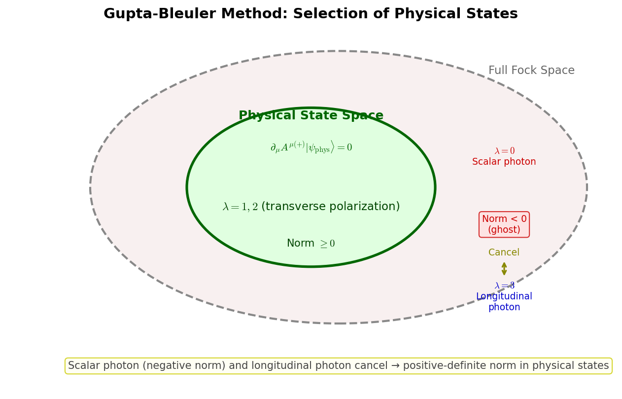
Fig. 6.4: Structure of the state space in the Gupta-Bleuler method. From the full Fock space, the physical state space is selected by the Gupta-Bleuler condition \(\partial_\mu A^{\mu(+)}|\psi_{\rm phys}\rangle = 0\). Scalar photons (negative norm) and longitudinal photons cancel, and positive-definite norm is restored for physical states.
🔵 Kai: It's reassuring that both methods give the same answer.
🟡 Lina: Right. This is the essence of gauge invariance—"the choice of gauge doesn't affect physical results."
✅ Comprehension Check: Explain in 2–3 sentences why negative-norm states appear in Lorenz gauge quantization and how the Gupta-Bleuler condition resolves this.
Answer
To maintain Lorentz covariance, quantizing all 4 components of \(A_\mu\) causes the scalar polarization (\(\lambda = 0\)) states to have negative norm due to the sign \(\eta_{00} = +1\) of the Minkowski metric. The Gupta-Bleuler condition \(\partial_\mu A^{\mu(+)}|\psi_{\text{phys}}\rangle = 0\) forces scalar and longitudinal photons to cancel within physical states, restoring positive-definite norm in the physical state space. As a result, physical photons are only the 2 transverse polarizations.
6.8 The Photon Propagator—Gauge Parameter \(\xi\)
🟡 Lina: For later chapters (Ch. 8 on Feynman diagrams), let's derive the photon propagator. The propagator represents the probability amplitude for a particle created at spacetime point \(x\) to propagate to another point \(y\). Mathematically, it's defined as the vacuum expectation value of the time-ordered product of field operators: \(\langle 0|T\{A_\mu(x)A_\nu(y)\}|0\rangle\). \(T\) is time-ordering—the operation of "placing later events to the left"—which intuitively automatically selects the causal order "photon born at \(x\), absorbed at \(y\) (or vice versa)." We'll learn this formally in Ch. 7. For now, let me just show the result. The photon propagator in Feynman gauge (\(\xi = 1\)) is
That is, in momentum space:
Here \(i\varepsilon\) (\(\varepsilon > 0\) is an infinitesimally small positive number) is a prescription to avoid the point where the denominator vanishes (\(k^2 = 0\), i.e., the photon is on-shell). Physically, it serves to select "causal propagation"—cause precedes effect. We'll learn the details in Ch. 7.
🔵 Kai: It looks similar to the scalar field propagator \(i/(k^2 - m^2 + i\varepsilon)\). It's like setting \(m = 0\) and multiplying by \(\eta_{\mu\nu}\). But if the propagator's form changes with different values of \(\xi\), how is it guaranteed that physical results stay the same?
🟡 Lina: Good question. Intuitively, the \(k_\mu k_\nu\) terms can be shown to always vanish in calculations of gauge-invariant physical quantities. For general \(\xi\):
For \(\xi = 1\) (Feynman gauge), the second term vanishes making it simple, which is why Feynman gauge is most commonly used in actual calculations.
⚪ Mei: Different values of \(\xi\) give the same physical scattering amplitudes—that's the consequence of gauge invariance.
🟡 Lina: Right. What guarantees the \(k_\mu k_\nu\) terms vanish is the Ward identity, which we'll study in detail in Ch. 9.
📝 Exercises:
- Fourier inverse transform of the photon propagator in Feynman gauge → Problem A-2. Lagrangian with Gauge-Fixing Term and the Photon Propagator
- Gupta-Bleuler condition and physical states → Problem M-3. Completeness Relation for Polarization Vectors
6.9 Why the Photon Is Massless—Protection by Gauge Symmetry
🟡 Lina: Finally, I want to convey a very deep message. Why is the photon massless?
🔵 Kai: Um... experimentally, the speed of light is finite, and if the photon had mass it would travel slower than light speed?
🟡 Lina: Experimentally that's correct. But the theoretical reason is much deeper. If we wanted to give the photon a mass \(m\), we would add a mass term to the Lagrangian:
This has the same structure as the scalar field mass term \(\frac{1}{2}m^2\phi^2\) from Ch. 4—quadratic in the field with coefficient proportional to \(m^2\). But look at how this behaves under gauge transformation (6.7):
Extra terms appear—it's not gauge invariant.
⚪ Mei: So gauge symmetry forbids the mass term. As long as gauge symmetry is preserved, the photon must be massless.
🟡 Lina: Exactly. This is an example of the deep principle that "symmetry determines physical laws." Conversely, if you want to give the photon a mass, you must break gauge symmetry in some way. This is the foreshadowing of the Higgs mechanism—the mechanism by which \(W\) and \(Z\) bosons acquire mass—which we'll learn in Ch. 19.
✅ Comprehension Check: Explain why the mass term \(\frac{1}{2}m^2 A_\mu A^\mu\) is incompatible with gauge symmetry.
Answer
Under gauge transformation \(A_\mu \to A_\mu + \partial_\mu \lambda\), we get \(A_\mu A^\mu \to A_\mu A^\mu + 2A^\mu \partial_\mu \lambda + (\partial_\mu \lambda)(\partial^\mu \lambda)\), with extra terms appearing that break invariance. Therefore adding a mass term to the Lagrangian breaks gauge symmetry, and as long as gauge symmetry is preserved, the photon mass must be zero.
🔵 Kai: Gauge symmetry is truly amazing. It demands the existence of force, protects the photon's zero mass... But wait. The \(W\) and \(Z\) bosons that carry the weak force have mass, right? If they're also derived from gauge symmetry, shouldn't they be massless?
🟡 Lina: A wonderful question. The resolution of that contradiction is the Higgs mechanism we'll learn in Ch. 19. By "spontaneously breaking" gauge symmetry, gauge bosons can acquire mass. And as we'll learn in Ch. 17, extending this principle to non-abelian groups (SU(2) and SU(3)) derives the weak and strong forces. The gauge principle is the central pillar supporting all of modern particle physics.
Summary—Comparison of Two Quantization Methods
🟡 Lina: Let's organize what we learned in this chapter.
Table 6.3: Comparison of quantization methods: Coulomb gauge and Lorenz gauge
| Coulomb Gauge | Lorenz Gauge + Gupta-Bleuler | |
|---|---|---|
| Gauge condition | \(\nabla \cdot \mathbf{A} = 0\) | \(\partial_\mu A^\mu = 0\) |
| Lorentz covariance | Not manifest | Manifest |
| Quantized degrees of freedom | 2 transverse polarizations only | All 4 polarizations |
| Negative norm problem | Doesn't arise | Arises → resolved by Gupta-Bleuler |
| Physical photons | 2 polarizations | 2 polarizations (selected by condition) |
| Computational convenience | Not suited for scattering calculations | Compatible with Feynman rules |
⚪ Mei: Both methods give the same final physics. The photon is massless, spin 1, with 2 transverse polarizations (helicity \(\pm 1\)). And all of this is derived from gauge symmetry—local U(1) invariance.
🔵 Kai: At first, hearing "redundancy" I thought it was just troublesome, but rather this redundancy governs the physics.
🟡 Lina: Right. Gauge symmetry: 1. Demands the existence of the electromagnetic field \(A_\mu\) (local U(1) → covariant derivative → \(A_\mu\)) 2. Uniquely determines the form of coupling to matter fields (\(\partial_\mu \to D_\mu\)) 3. Protects the photon's zero mass (mass term is not gauge invariant) 4. Restricts physical degrees of freedom to 2 (4 components → 2 polarizations)
🔵 Kai: All this from a single principle... But U(1) is just a "phase rotation"—a simple group. What changes fundamentally when you extend to SU(2) or SU(3)?
🟡 Lina: A crucial question. U(1) is an abelian group—the order of transformations doesn't matter. But SU(2) and SU(3) are non-abelian groups where the order of transformations changes the result. As a consequence, the gauge field itself carries "charge" and gauge fields interact with each other. Photons carry no charge, so photons don't directly interact with each other, but gluons (particles carrying the strong force) carry "color charge" and interact with each other. This is the essence of Yang-Mills theory, which describes all forces in nature (except gravity). We'll study this in detail in Ch. 17. Fig. 6.5 "Comparison of gauge-fixing methods. Coulomb gauge versus Lorenz gauge + Gupta-Bleuler. The approaches differ, but the final conclusion is the same" summarizes the overall picture of the two quantization methods.
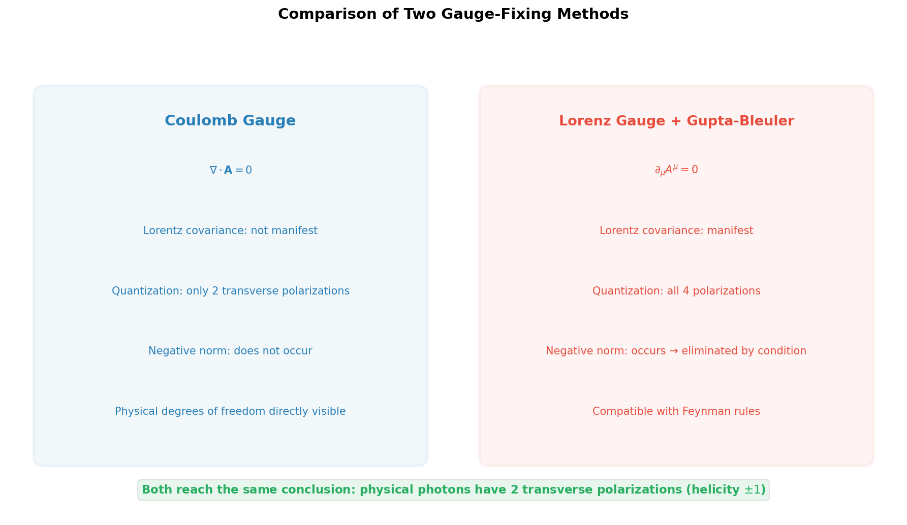
Fig. 6.5: Comparison of gauge-fixing methods. Coulomb gauge versus Lorenz gauge + Gupta-Bleuler. The approaches differ, but the final conclusion is the same—physical photons have 2 transverse polarizations.
✅ Comprehension Check: List the 4 roles that gauge symmetry plays for the photon.
Answer
(1) The requirement of local U(1) symmetry leads to the existence of the electromagnetic field \(A_\mu\). (2) The covariant derivative \(D_\mu = \partial_\mu + iqA_\mu\) uniquely determines the form of coupling to matter fields. (3) Since the mass term \(m^2 A_\mu A^\mu\) is not gauge invariant, the photon's zero mass is protected. (4) The redundancy of gauge transformations restricts the physical degrees of freedom of the 4-component vector field to 2 transverse polarizations.
6.10 Connection to the Maxwell Field Learned in Quantum Mechanics
🟡 Lina: Finally, let's confirm the connection to what we learned in Quantum Mechanics Ch. 27. In that chapter, we previewed the picture that "oscillation modes of a field are particles."
🔵 Kai: Yes. The story was "just as vibration modes of a violin string become sound, oscillation modes of a field become particles." But if a classical electromagnetic wave is "a state where many photons oscillate together," how exactly does a single-photon state differ from a classical wave state?
🟡 Lina: Good question. A single-photon state \(|1_{\mathbf{k},\lambda}\rangle\) has zero expectation value of the electric field, and each measurement gives a random value—the photon number is definite but the electric field "amplitude" is uncertain. On the other hand, what corresponds to a classical electromagnetic wave is a special state called a "coherent state." Imagine a state where the photon number is uncertain but the electric field amplitude and phase are nearly definite—laser light is close to this.
🔵 Kai: Huh, laser light is a "coherent state"... That's a special quantum mechanical state.
🟡 Lina: Mathematically, it's defined as an eigenstate of the annihilation operator \(a\) (\(a|\alpha\rangle = \alpha|\alpha\rangle\), where \(\alpha\) is a complex number). In Quantum Mechanics Ch. 9 we learned that for the harmonic oscillator, \(\hat{a}|n\rangle = \sqrt{n}|n-1\rangle\)—number states \(|n\rangle\) are not eigenstates of \(\hat{a}\). A coherent state is a superposition of number states \(|\alpha\rangle = e^{-|\alpha|^2/2}\sum_n \frac{\alpha^n}{\sqrt{n!}}|n\rangle\), a special state whose "shape doesn't change" when \(\hat{a}\) acts on it. Since \(\hat{a}\) is not Hermitian, the eigenvalue \(\alpha\) can be complex rather than real.
🔵 Kai: "The state's shape doesn't change when the annihilation operator acts"—does that mean removing one photon leaves the state the same?
🟡 Lina: Yes, intuitively that's exactly it. Like scooping one cup of water from a bucket barely changes the water level—since there are so many photons, removing one doesn't change the overall "shape." \(|\alpha|^2\) represents the average photon number, and the phase of \(\alpha\) corresponds to the phase of the electric field. When the average photon number is very large, the expectation value of the electric field approaches the classical wave form \(E_0 \cos(\omega t - \mathbf{k}\cdot\mathbf{x})\). The precise mathematical definition belongs to quantum optics, but for now remember that "classical electrodynamics is recovered in the limit of large photon numbers."
🔵 Kai: I see. A single-photon state is "definite particle number but uncertain field value," while a classical wave is "nearly definite field value but uncertain particle number"—they're exactly opposite.
⚪ Mei: Particle number and phase have a complementary relationship like uncertainty. The "position and momentum" structure from quantum mechanics lives on in field theory.
🟡 Lina: In this chapter, we realized field quantization for the electromagnetic field. We decomposed the classical Maxwell field into Fourier modes and quantized each mode as a quantum mechanical harmonic oscillator. The results:
- Each mode \((\mathbf{k}, \lambda)\) excitation is "a photon with momentum \(\mathbf{k}\) and polarization \(\lambda\)"
- \(n\) excitations → \(n\) photons (Fock space)
- Classical electromagnetic wave → coherent state of many photons
⚪ Mei: So Maxwell's classical electrodynamics is recovered as the limit of large photon numbers.
🟡 Lina: Right. This completes the quantization of free fields for spin 0 (Ch. 4), spin 1/2 (Ch. 5), and spin 1 (this chapter). Starting from the next chapter, we'll finally mix these fields—introducing interactions.
Preview of the Next Chapter
With free fields of spin 0, 1/2, and 1 in hand, we now enter the stage of "mixing" fields together. In Ch. 7, we add interaction terms to the Lagrangian and formulate the S-matrix for systematically describing scattering processes. Armed with the Dyson series and time-ordered products, we'll unravel the structure of perturbative expansion and open the door to that powerful computational tool—Feynman diagrams.
References
- Quantum Field Theory for the Gifted Amateur (Lancaster & Blundell) Chapter 14, "Gauge Invariance and the Electromagnetic Field"
- David Tong, Quantum Field Theory Lecture Notes Chapter 7, "Quantizing the Electromagnetic Field"
- 場の量子論:不変性と自由場を中心にして(場上) Chapter 3, "Relativistic Form of Maxwell's Equations and Gauge Invariance"
- 場の量子論:不変性と自由場を中心にして(場上) Chapter 7, "The Gauge Principle — Force Born from Symmetry"
- 場の量子論:不変性と自由場を中心にして(場上) Chapter 13, "Quantization of the Maxwell Field — The Struggle with Gauge Freedom"
- Quantum Field Theory and the Standard Model (Schwartz) Chapter 6, "Spin 1 and Gauge Invariance"
- Quantum Field Theory and the Standard Model (Schwartz) Chapter 7, "Scalar QED"
Feedback on this page
Let us know if something was unclear, incorrect, or could be improved.