Prologue: Welcome to This Journey — Motivation and the Overall Map¶

← Ch. 28 The Quantum Gravity Pr…Ch. 1 Why Quantum Field Theor… →

Before You Begin

If you haven't read it yet, please start with Introduction — Before the Four Journeys. There you can find the philosophical stance shared across this entire site (models are hypotheses / equations are tools for falsifiability) and the map of the four journeys.

Goals of This Prologue

Gain an intuitive grasp of "what QFT describes as a model" — Get a taste of the worldview where particles are understood as excitations of fields
Obtain the map of all 24 chapters — Welcome readers who have finished quantum mechanics, and survey the role of each Part
Preview the bridge to the final destination — Keep in mind that Ch. 24 connects to The Quest for Quantum Gravity

Welcome Back — To Those Who Completed the Quantum Mechanics Journey¶

🟡 Lina: ……Well then. You two, congratulations on completing the quantum mechanics journey.

🔵 Kai: Man, that was long! Including the prologue, 28 chapters... Toward the end, my head was about to explode.

⚪ Mei: But in the final chapter, we were told "there's an even bigger world beyond this," and honestly, I've been curious ever since.

🟡 Lina: Do you remember what we discussed in the final chapter, Quantum Mechanics Ch. 27? "The Schrödinger equation cannot treat time and space on equal footing. When you try to reconcile special relativity with quantum mechanics, phenomena where the number of particles changes become unavoidable"——

🔵 Kai: I remember. We derived the Klein-Gordon equation and the Dirac equation, and went as far as predicting antiparticles. But at the end, we were told "this is only the entrance. The real story is in quantum field theory," and that's where it ended.

🟡 Lina: Right. At that time, I previewed the worldview that "vibrational modes of a field are particles." Starting today, we begin a journey of pursuing that worldview with equations. Let me remind you — in quantum mechanics, the number of particles was fixed. One electron, two electrons... you decided the particle number first, then solved the equation.

⚪ Mei: Yes. When setting up the Schrödinger equation, we always decided "how many particles" first, then wrote the wave function.

🟡 Lina: Exactly. But in the real world — when electrons and positrons collide inside an accelerator, photons are born, muon pairs fly out, Higgs particles appear. Particles are created and destroyed. Within the framework of quantum mechanics, we couldn't properly handle this phenomenon of "changing numbers."

🔵 Kai: And what handles that is quantum field theory... right?

🟡 Lina: Yes. But quantum field theory isn't merely "a tool for describing particle creation and annihilation." It's a more fundamental shift in worldview.

🔵 Kai: A shift in worldview?

🟡 Lina: In quantum mechanics, "particles" were the protagonists, right? There's a particle called the electron, and it behaves according to a wave function. But in quantum field theory, the protagonist is the field. There's a "field" spread across all of space in the universe, and when that field vibrates in a specific way — one unit of that vibration is observed as a "particle."

🔵 Kai: What do you mean by "one unit of vibration"? Is it related to how energy becomes discrete in increments of \(\hbar\omega\) in the quantum mechanical harmonic oscillator?

🟡 Lina: Exactly that. In the quantum mechanical harmonic oscillator, energy was quantized in integer multiples of \(\hbar\omega\), right? In quantum field theory, each vibrational mode of the field is a harmonic oscillator, and "one energy step" corresponds to one particle. We'll follow the equations in detail in Ch. 4, but for now just hold onto this image.

⚪ Mei: So... particles are a concept that "derives from" the field?

🟡 Lina: Yes. Imagine a calm pond. The entire water surface corresponds to the "field." When you throw a stone in, ripples spread out, right? Each of those ripples is a "particle." The water surface (field) exists everywhere in the universe from the start, and ripples (particles) appear and disappear — that's the worldview of quantum field theory. In the conventional picture, particles were treated as independent "points," and even in quantum mechanics, particle number was fixed. In quantum field theory, both of these change. Fig. 0.1 "The particle picture versus the quantum field theory picture. Left" summarizes the difference between the two pictures, so take a look.

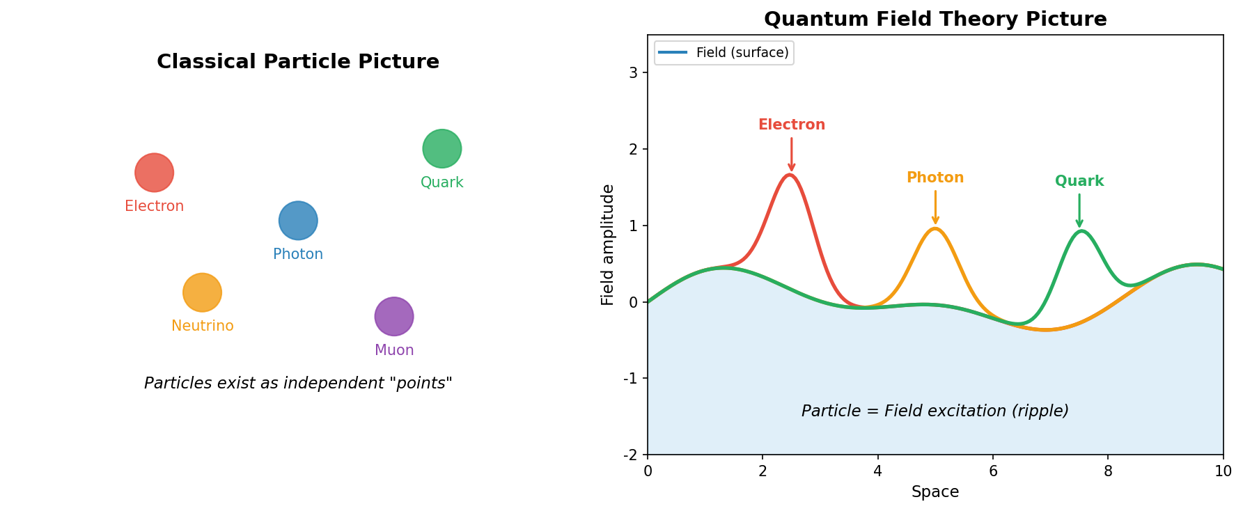
Fig. 0.1: The particle picture versus the quantum field theory picture. Left — In the conventional particle picture, particles exist as independent "points" (particle number is fixed even in quantum mechanics). Right — In quantum field theory, excitations (ripples) of a "field" spread across the entire universe are observed as particles.

🔵 Kai: Wow... So all electrons are vibrations of the same "electron field"?

🟡 Lina: Yes. That's precisely why, no matter where in the universe you measure, the electron mass is \(0.511\ \mathrm{MeV}/c^2\), the charge is \(-e\), and the spin is \(1/2\). All electrons are perfectly identical because they are the same type of vibration of the same field. Bolts made in a factory look slightly different under a microscope, but electrons are truly perfectly identical. Quantum field theory answers the "why" of this.

✅ Comprehension Check: In quantum field theory, explain in the language of "fields" why every electron in the universe is perfectly identical.

Answer

All electrons are the same type of excitation (vibrational mode) of the identical "electron field," so properties such as mass, charge, and spin are perfectly identical. The identity of particles is naturally explained by the fact that they arise from the same field.

🔵 Kai: But are electrons in Tokyo and electrons in New York really "the same" even though they're in different places?

🟡 Lina: Good question. The locations are different, but the type — "which vibrational mode of the electron field was excited" — is the same. Even if you pluck the first string of a guitar in Tokyo or in Osaka, the same pitch comes out, right? The location is different, but because the string's properties are the same, the same note sounds — it's a similar idea. We'll confirm this with equations in Ch. 4.

Four Wonders That Quantum Field Theory Addresses¶

🟡 Lina: Now, we're going to spend 24 chapters learning quantum field theory, but first let me show you "what this theory can explain" through four concrete examples. No equations yet. Today is just about tasting the "amazingness." Let me state the four upfront — (1) ultra-precise calculation of the electron's magnetic moment, (2) particle creation and annihilation at accelerators, (3) superconductivity, (4) fluctuations at the beginning of the universe. I want you to feel the breadth of coverage, from the microscopic to the macroscopic.

Wonder 1: The Anomalous Magnetic Moment of the Electron — The Most Precise Agreement in Human History¶

🟡 Lina: In quantum mechanics, you learned that the electron's spin undergoes precession in a magnetic field — a wobbling motion like a spinning top, where the spin direction rotates around the magnetic field. The electron's magnetic moment (its strength as a magnet) is proportional to its spin angular momentum. Here, "magnetic moment" is a quantity representing the magnetic strength of a current loop, defined as "current × loop area." In equation form:

\[ \boldsymbol{\mu} = -g\,\frac{e}{2m_e}\,\mathbf{S} \]

Here \(e\) is the elementary charge, \(m_e\) is the electron mass, and \(\mathbf{S}\) is the spin angular momentum. The dimensionless number \(g\) appearing in this proportionality coefficient is the "\(g\)-factor."

🔵 Kai: Is the \(g\)-factor like a "magnification factor" for the magnetic moment? If \(g = 1\) it's normal, and \(g = 2\) means it's twice as strong a magnet?

🟡 Lina: Good question. Let me confirm the classical reference value. The elementary charge \(e\) is a positive constant (\(e > 0\)), and the electron's charge is \(-e\) — that is, "minus one times" the elementary charge. For now, let's ignore the sign and consider a particle with charge magnitude \(e\) and mass \(m_e\) moving at speed \(v\) in a circular orbit of radius \(r\) (here we only want the magnitude of the magnetic moment, so don't worry about the current direction being opposite to the electron's direction of motion). The magnitude of the orbital angular momentum is \(L = m_e v r\). Now, since this particle goes around the circular orbit periodically, if you watch a given cross-section, the charge \(e\) passes through it once every revolution — this is the same as "current flowing."

🔵 Kai: Ah, I see. Just like electrons flowing through a wire, "the amount of charge passing through a cross-section per unit time" is the definition of current, so a particle orbiting creates a current.

🟡 Lina: Exactly. The period is \(T = 2\pi r/v\), so the current (charge passing per unit time) is \(I = e/T = ev/(2\pi r)\). The area enclosed by this current loop is \(\pi r^2\), so from the definition of magnetic moment "current × area," we get \(\mu = I \cdot \pi r^2 = evr/2\).

⚪ Mei: With \(\mu = evr/2\) and \(L = m_e v r\)... if we take the ratio of \(\mu\) and \(L\), both \(v\) and \(r\) cancel out, leaving only constants.

🔵 Kai: Um... so I just need to take the ratio of \(\mu\) and \(L\), right?

🟡 Lina: Yes. \(\mu/L = (evr/2)/(m_e v r) = e/(2m_e)\), which corresponds to \(g = 1\) — meaning for classical orbital motion, \(g = 1\) is the natural value. By the way, the minus sign in the original equation \(\boldsymbol{\mu} = -g\,\frac{e}{2m_e}\,\mathbf{S}\) indicates that because the electron's charge is \(-e\) (negative), the magnetic moment points antiparallel to the spin. The \(g\)-factor itself is a positive number representing "how many times the classical reference \(e/(2m_e)\)."

⚪ Mei: For orbital motion, \(g = 1\). But for spin, it's different, right?

🟡 Lina: Exactly. The Dirac equation predicts that for the electron's spin, \(g\) is exactly \(2\) — twice the classical orbital motion value. To give one-line intuition for why it's doubled: the relativistic structure of the Dirac equation (the 4-component spinor structure) doubles the coupling between spin and the magnetic field compared to the classical expectation. This was the first nontrivial result explained by relativistic quantum mechanics.

⚪ Mei: Yes. We saw in Quantum Mechanics Ch. 27 that \(g = 2\) emerges naturally from the Dirac equation.

🟡 Lina: But when you measure precisely in experiments, \(g\) is not exactly \(2\) — it deviates from \(2\) by a tiny amount. This deviation is called the "anomalous magnetic moment." Using quantum field theory — specifically QED (Quantum Electrodynamics) — you can calculate this deviation.

🔵 Kai: How precise is it?

🟡 Lina: The theoretical and experimental values agree to 10 decimal places.

🔵 Kai: ...10 digits!? But wait. Doesn't the fact that \(g\) isn't exactly \(2\) mean the Dirac equation is wrong?

🟡 Lina: Good question. The Dirac equation gives the answer for the case where "the electron doesn't interact with anything else." But a real electron is constantly interacting with the surrounding electromagnetic field — including its quantum fluctuations. That deviation appears in \(g - 2\). As an analogy, it's like measuring the distance from the Earth to the Sun — about 150 million km — with not even 1 cm of error. That's the level at which theory and experiment agree.

🟡 Lina: QED is the most precisely experimentally confirmed physical model humanity has ever created. Take a look at Fig. 0.2 "Precision comparison of physical models" — you can see at a glance that compared to predictions of Newtonian mechanics, general relativity, and other Standard Model predictions, the precision is orders of magnitude better.

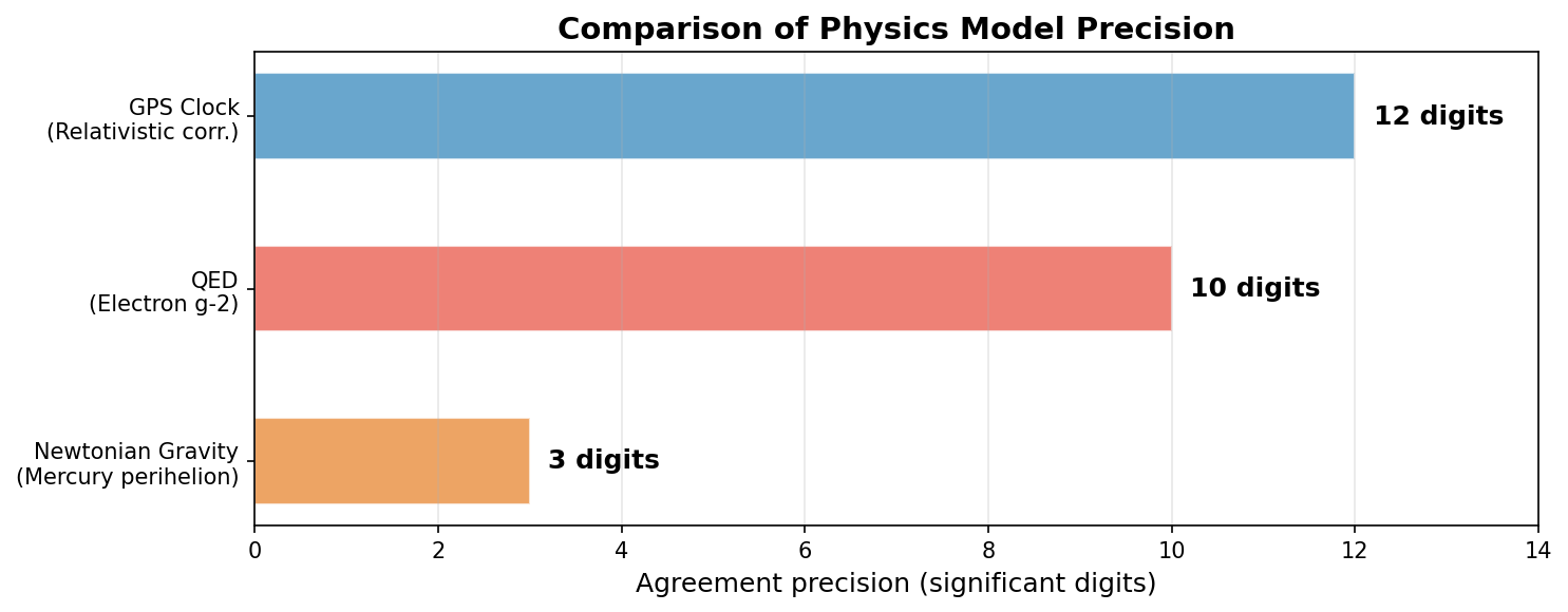
Fig. 0.2: Precision comparison of physical models. Agreement between theoretical and experimental values for various physical models. The electron g-2 in QED agrees to 10 decimal places, making it the most precisely tested model in human history.

🔵 Kai: Measuring from the Earth to the Sun with not even 1 cm of error... It's amazing that they can tell it's "not exactly \(2\)" despite such agreement. How do you calculate it?

🟡 Lina: The electron virtually emits and reabsorbs a photon, then that photon creates a virtual electron-positron pair... You systematically add up all such "quantum fluctuations" using pictures called Feynman diagrams. In Chapters 8–9 of this book, we'll learn that method.

⚪ Mei: So the deviation from \(g = 2\) is the effect of "how the electron interacts with the surrounding electromagnetic field," and the tool for systematically calculating that is what Lina calls Feynman diagrams.

🔵 Kai: Are "virtual photons" different from real photons?

🟡 Lina: Good question. Virtual particles aren't directly observed — they're like "intermediate states" that appear in the middle of a calculation. They exist for just the short time that the uncertainty principle allows, then disappear — that's the image. The precise definition comes in Ch. 7, so for now just think of them as "invisible but having real effects."

🔵 Kai: "Invisible but having real effects" sounds kind of like ghosts... But if the calculation matches to 10 digits, I guess they really "exist." But what I'm wondering is — do virtual particles "actually exist," or are they "just a convenient calculation tool"?

🟡 Lina: That's a sharp question. It's actually debated among physicists. At minimum, we can say that since calculations including virtual particles agree with experiment to 10 digits, the calculation method provides a "correct description." How you define "existence" is partly a philosophical question — but in this journey, we'll proceed with the stance of "using them systematically as computational tools and comparing with experiment." Don't worry, we'll go step by step.

✅ Comprehension Check: In the language of quantum field theory, what causes the electron's \(g\)-factor to deviate from exactly \(2\)?

Answer

The existence of "quantum corrections (loop corrections)" where the electron interacts with virtual photons and virtual electron-positron pairs.

Wonder 2: Particle Creation and Annihilation — The World Revealed by Accelerators¶

🟡 Lina: The second example is accelerator experiments. At CERN's LHC (Large Hadron Collider), protons are accelerated to 99.9999991% of the speed of light and smashed together.

🔵 Kai: What happens when they collide at such speeds?

🟡 Lina: The kinetic energy released in the collision gets converted into the mass of new particles, following the relation \(E = mc^2\) — energy and mass are equivalent. Particles that didn't exist before the collision are created in abundance. The Higgs particle discovered in 2012 was born this way. You just collide two protons, yet a particle more than 130 times heavier than a proton appears.

⚪ Mei: So the kinetic energy of the collision is converted into the mass of new particles.

🟡 Lina: Right. And calculating this process quantitatively — "what's the probability that a Higgs particle is produced?" "what angular distribution do the decay products fly off in?" — all of this is quantum field theory calculation. In Chapters 17–21 of this book, we'll learn the structure of the Standard Model.

🔵 Kai: The Standard Model is the model that puts together all the fundamental forces and particles in nature, right?

🟡 Lina: Yes. It's the model that describes the electromagnetic force, weak force, and strong force — three fundamental forces excluding gravity — along with quarks, leptons, gauge particles, and the Higgs particle in a unified framework. And its mathematical language is quantum field theory.

Wonder 3: Superconductivity — Quantum Field Theory Isn't Just for Particle Physics¶

🟡 Lina: Third example. You don't think quantum field theory is only for particle physics, do you?

🔵 Kai: Wait, it isn't?

🟡 Lina: Not at all. Consider superconductivity — the phenomenon where certain metals, when cooled to extremely low temperatures, have their electrical resistance drop to zero. The BCS theory (Bardeen–Cooper–Schrieffer theory, named after three physicists) that microscopically explains this shows that electrons pair up and behave collectively, resulting in zero resistance. And this theory is constructed using the tools of quantum field theory — specifically a mechanism called "spontaneous symmetry breaking."

🔵 Kai: Hold on. Electrons have negative charge, so they should repel each other, right? How can they pair up? And why does pairing lead to zero resistance?

🟡 Lina: Good questions, but explaining everything here would take too long, so let me just convey the image for now. First, "why can they pair up" — the electrons don't directly stick together. Instead, they attract each other indirectly through crystal lattice vibrations. When the first electron passes through, the lattice slightly distorts, and that distortion attracts the second electron — there's a "mediator" in between. Next, "why does resistance become zero" — when a large number of pairs gather and all "condense" into the same quantum state, the entire collective behaves as one giant wave. If you try to scatter just one, you'd have to move the entire collective, so small obstacles can't scatter them — hence zero resistance. We'll cover the details in Ch. 22. Today's point is that quantum field theory tools are used in that theory.

🔵 Kai: Got it. So what is "symmetry breaking"?

🟡 Lina: Simply put, it's a phenomenon where the laws themselves are left-right symmetric, but the state that's actually realized is biased to one side. If you balance a pencil vertically on a table, it could fall in any direction, but it actually falls in one direction, right? That's an analogy for "symmetry breaking."

🔵 Kai: But isn't that just determined by wind or hand trembling? If the laws are symmetric, what "breaks" it?

🟡 Lina: Good question. The key point isn't "which direction it falls" but "it can't stay standing." The symmetric state (pencil standing upright) is energetically unstable, and the system inevitably settles into an asymmetric state (fallen over). Which direction it falls is random, but "the fact that it falls" is demanded by the laws. Details in Ch. 18.

🟡 Lina: Actually, this means that the same mathematical structure is shared between the world of particle physics and the world of condensed matter physics. The tools of quantum field theory were created to describe elementary particles, but their mathematical structure — symmetry and its breaking — doesn't depend on scale, so they can also be applied to condensed matter physics. Moreover, historically, the idea of "spontaneous symmetry breaking" discovered in condensed matter physics was reverse-imported into particle physics, giving birth to the Higgs mechanism — the mechanism by which particles acquire mass. In Chapters 18–19 and Ch. 22, we'll see this beautiful connection.

⚪ Mei: So the key point is the universality of the tools — the same mathematics can be used across scales.

🔵 Kai: The same structure appearing across fields is pretty cool. But particle physics and electrons in metals are at completely different scales — why can the same math be used?

🟡 Lina: Good question. The phenomenon of "symmetry breaking" can occur regardless of scale. If the structure of the laws is the same, the same mathematics applies — this is a prime example demonstrating the universality of quantum field theory.

Wonder 4: Fluctuations in the Cosmic Microwave Background — The Fingerprint of the Universe's Beginning¶

🟡 Lina: The last example is cosmology. Have you heard of the Cosmic Microwave Background (CMB)?

🔵 Kai: That's like the afterglow of the Big Bang, right? No matter which direction you look in the universe, radiation at almost the same temperature comes in.

🟡 Lina: Right. But "almost the same" — not perfectly uniform. There are tiny temperature variations — fluctuations — at the level of one part in 100,000. The pattern of these fluctuations became the "seeds" that later grew into galaxies and galaxy clusters.

⚪ Mei: What's the origin of those fluctuations?

🟡 Lina: In the current standard model, during the very early universe — an era called inflation, a period of rapid expansion — vacuum fluctuations of quantum fields were stretched out and became density fluctuations on cosmic scales.

🔵 Kai: Vacuum fluctuations? Isn't vacuum supposed to mean "nothing is there"? Why are there fluctuations?

🟡 Lina: Remember the uncertainty principle from quantum mechanics. Just as position and momentum have the relation \(\Delta x \cdot \Delta p \gtrsim \hbar/2\), there's an analogous relation between energy and time: \(\Delta E \cdot \Delta t \gtrsim \hbar/2\). The important conclusion here is that "a state of perfectly zero energy is not allowed" — on very short time scales, energy necessarily fluctuates. These are vacuum fluctuations.

By the way, let me add one note for accuracy: unlike the position-momentum case, there's no "time operator," so \(\Delta E \cdot \Delta t \gtrsim \hbar/2\) isn't strictly the same kind of uncertainty relation. The precise meaning is "a state with a large energy spread can change in a shorter time" — but what matters for our discussion is just the conclusion that "even in vacuum, energy can never be perfectly zero." As a qualitative image, understanding it as "on short time scales, energy can fluctuate significantly" is sufficient. The rigorous derivation will naturally emerge in Ch. 4 when we quantize the field.

🔵 Kai: Those quantum mechanical fluctuations became the seeds of the entire universe's structure...?

🟡 Lina: Yes. Microscopic quantum fluctuations giving birth to macroscopic cosmic structure — this is a topic at the intersection of quantum field theory and general relativity, which we'll touch on in Ch. 24.

✅ Comprehension Check: How is the origin of the tiny temperature fluctuations seen in the Cosmic Microwave Background (CMB) explained from the perspective of quantum field theory?

Answer

During the very early universe (the inflationary period), vacuum fluctuations of quantum fields (fluctuations arising from the fact that the uncertainty principle prevents energy from being zero even in vacuum) were stretched by the rapid cosmic expansion and became density fluctuations on cosmic scales. These are observed as temperature variations in the CMB.

🔵 Kai: From the magnetic moment of a single electron to the structure of the entire universe... that's quite a range.

🟡 Lina: Yes. The electron scale is about \(10^{-15}\) m, and the large-scale structure of the universe is about \(10^{26}\) m — phenomena spanning more than 40 orders of magnitude in scale can be described within the same theoretical framework. That's the power of quantum field theory.

⚪ Mei: More than 40 orders of magnitude... It's amazing that a single theory can cover such a wide range. But I want to keep in mind the stance we shared in the Introduction — models are hypotheses, and equations are tools for falsifiability.

🟡 Lina: That's a good mindset. Now, keeping that awareness, let's survey the overall map of our journey.

Roadmap of All 24 Chapters — The Complete Journey Map in 7 Parts¶

🟡 Lina: Now, let's survey the overall map of our journey. I'll introduce all 24 chapters divided into 7 Parts, presented as a narrative.

🔵 Kai: 24 chapters... that's a long journey.

🟡 Lina: Don't worry. Since each Part builds upon the previous one, if you proceed in order you'll definitely reach the end. After I've introduced all the Parts, the overall overview is summarized in Fig. 0.4 "Roadmap of all 24 chapters", and the chapter structure and keywords for each Part are in Table 0.1 "Overview of chapter structure and keywords for all 7 Parts". If you ever get lost, come back here. Let's go through them Part by Part.

Part I: Review and Classical Fields (Chapters 1–3) — Preparing for the Journey¶

🟡 Lina: The first 3 chapters are "preparation."

Ch. 1 "Why Quantum Field Theory Is Needed" starts from where Quantum Mechanics Ch. 27 left off, reorganizing why the quantum mechanics of particles is insufficient.
Ch. 2 "Review of Special Relativity and Lorentz Invariance" prepares the tools of special relativity — 4-vectors, Lorentz transformations, invariant intervals — in the form needed for quantum field theory. This chapter is self-contained, so it's fine even if you haven't read General Relativity. For those who've read Chapters 3–4 of General Relativity, this chapter reorganizes those tools for field theory.
Ch. 3 "Classical Field Theory" covers the Lagrangian of classical fields and Noether's theorem before quantizing the field. This theorem, which derives conserved quantities from symmetries, is the most important tool throughout the entire journey.

⚪ Mei: We learned about the relationship between symmetries and conservation laws in quantum mechanics too, but how does it change in field theory?

🟡 Lina: In field theory, "there are as many conserved quantities as there are continuous symmetries" can be automatically read off from the structure of the Lagrangian. It becomes more systematic and more powerful than in quantum mechanics.

⚪ Mei: I see, so the correspondence between symmetries and conserved quantities emerges automatically from the Lagrangian. That sounds exciting.

🟡 Lina: Yes. We'll verify it hands-on in Ch. 3.

Part II: Canonical Quantization of Free Fields (Chapters 4–6) — Particles Are Born from Fields¶

🟡 Lina: Part II is the first major peak of this journey. Here we learn the core operation of "quantizing the field."

Ch. 4 "Quantization of the Scalar Field" — We quantize the simplest field (a "scalar field" with no spin, i.e., spin 0) and see that creation operators \(\hat{a}^\dagger\) and annihilation operators \(\hat{a}\) naturally emerge. "Scalar" means a quantity represented only by magnitude with no "direction" — like a temperature distribution assigning a temperature to each point in space, whose value at each point doesn't change when you rotate the coordinate system or switch to the reference frame of a moving observer (the precise definition comes in Ch. 2). The creation and annihilation operators of the harmonic oscillator you learned in quantum mechanics reappear here as operators that "create and destroy particles."
Ch. 5 "Quantization of the Dirac Field" — Handling spin-\(1/2\) fermions. Instead of the commutation relations (\(AB - BA = \text{something}\)) used in quantum mechanics, we impose anticommutation relations (\(AB + BA = \text{something}\)).

🔵 Kai: Huh, why won't commutation relations work? We always used commutation relations in quantum mechanics.

🟡 Lina: If you impose commutation relations on fermions, you could put any number of particles in the same state, contradicting the Pauli exclusion principle. To automatically satisfy the exclusion principle, anticommutation relations are needed. Specifically, we require for the creation operators: \(\{\hat{a}_i^\dagger,\, \hat{a}_j^\dagger\} \equiv \hat{a}_i^\dagger \hat{a}_j^\dagger + \hat{a}_j^\dagger \hat{a}_i^\dagger = 0\). Here the curly braces \(\{\cdot,\cdot\}\) denote the anticommutator — different from the set notation in high school math, it's the "\(+\) version" corresponding to the commutator \([A,B] = AB - BA\). The formal introduction is in Ch. 5. Let me give just the intuition for why this alone yields the exclusion principle — if you write the operation of putting a particle into the same state \(i\) twice as \((\hat{a}_i^\dagger)^2\), then setting \(i = j\) in the above equation gives \(\hat{a}_i^\dagger \hat{a}_i^\dagger + \hat{a}_i^\dagger \hat{a}_i^\dagger = 2(\hat{a}_i^\dagger)^2 = 0\), meaning \((\hat{a}_i^\dagger)^2 = 0\). This means that if you try to create a "state with 2 particles in the same state," the result is the zero vector. Do you remember what the zero vector means? In quantum mechanics, the square of the magnitude of a state vector was "the total probability of that state being realized." If the magnitude is zero, the probability is also zero — so the zero vector represents "a physically unrealizable state." Therefore "trying to put 2 particles in the same state gives a physically forbidden state" — the Pauli exclusion principle (no more than one fermion can occupy the same quantum state) is mathematically built in. - Ch. 6 "Quantization of the Electromagnetic Field" — Describing photons. Here we'll wrestle with the tricky problem of "gauge freedom."

🔵 Kai: So the reason we studied the harmonic oscillator so carefully in quantum mechanics finally becomes clear here. But one thing I'm wondering — the harmonic oscillator was "one oscillator," right? Since the field exists at every point in space, does that mean there are infinitely many oscillators? Is that okay?

🟡 Lina: Good question. That's right — each mode of the field is an independent harmonic oscillator, and there are infinitely many of them. The question "is it okay to have infinitely many" is actually a deep problem directly connected to renormalization (Part V). But for now, just take comfort in knowing that "each mode is the same harmonic oscillator you learned in quantum mechanics." The quantum mechanical harmonic oscillator was the shortest bridge to quantum field theory.

Part III: The First Reward — QED (Chapters 7–9)¶

🟡 Lina: Part III is where we "actually calculate" using the tools we've built so far.

Ch. 7 "Interactions and the S-Matrix" — Learning how to "mix" free fields together. Building the framework for treating interactions as perturbations and calculating scattering amplitudes.
Ch. 8 "Feynman Diagrams" — Learning the "pictures" that are the symbol of quantum field theory. Simple pictures made of lines and vertices translate one-to-one into complex equations.
Ch. 9 "Basic Processes in QED" — Actually calculating electron-photon scattering (Compton scattering, Rutherford scattering, etc.) and comparing with experiment. Here you'll experience for the first time that "quantum field theory really works."

🔵 Kai: Can Fermi's golden rule and perturbation theory that we learned in quantum mechanics be used here too? Even though the particle number changes?

🟡 Lina: Good question. They reappear not "as is" but extended as the field theory versions. But the backbone is the same, so your quantum mechanics knowledge directly applies. Specifically, the structure of calculating transition probabilities as "initial state → interaction → final state" is shared with quantum mechanics. However, in quantum field theory, the types and numbers of particles in the initial and final states can change — that's the part that gets extended.

⚪ Mei: I see. The "backbone" of the calculation is the same as quantum mechanics, but the framework is broadened to handle processes where particle numbers change.

🔵 Kai: But wait. If particles are created and destroyed along the way, the particle numbers in the "initial state" and "final state" are different, right? How do you define the transition probability in that case?

🟡 Lina: That's a question that hits the core. The one-word answer is: the tool that defines "transition amplitudes between initial and final states with different particle numbers" is the S-matrix. Using creation and annihilation operators, we can handle "states with different particle numbers" within the same framework — we'll learn that mechanism head-on in Ch. 7.

Part IV: Path Integrals (Chapters 10–12) — Another Way to Quantize¶

🟡 Lina: In Part IV, we learn a different approach to quantization.

Ch. 10 "Path Integrals in Quantum Mechanics" — Introducing Feynman's path integral, first within the scope of quantum mechanics. The picture is "the particle simultaneously takes all possible paths, and we sum up their amplitudes."
Ch. 11 "Path Integrals for Fields and Generating Functionals" — Extending path integrals to fields. This gives us a formulation of quantum field theory from a different angle than canonical quantization.
Ch. 12 "Path Integrals for Fermions" — Handling fermions in path integrals requires special mathematics called Grassmann numbers. Unlike ordinary numbers, they "square to zero" — the same spirit as the anticommutation relations from earlier.

🔵 Kai: Squaring to zero!? Do such numbers exist...? But it's the same mechanism as \((\hat{a}_i^\dagger)^2 = 0\) from earlier. That's fine, but why are there two methods of quantization?

🟡 Lina: Each has its strengths. Canonical quantization gives a clear physical picture but makes gauge theories cumbersome to handle. Path integrals have excellent compatibility with gauge theories and are also suited for phenomena invisible to perturbative expansion — the method of approximating by assuming the interaction strength is weak. Non-perturbative phenomena are things like "tunnel effects where the field configuration changes dramatically" — we'll see concrete examples in Part VII. Knowing both lets you choose the right tool for the problem.

🔵 Kai: You get the same answer but go through the trouble of doing it two ways? Can't you just use one?

🟡 Lina: It's like climbing the same mountain by different routes. The scenery invisible from the north face can be seen from the south face. In fact, there are theorems that can only be proven using path integrals.

🔵 Kai: I see... If "there's scenery that can only be seen from one side," then there's meaning in doing both. What's a specific example of "scenery visible only from the path integral"?

🟡 Lina: For example, "instantons" covered in Ch. 23 — phenomena where the field configuration tunnels dramatically — can't be naturally described without the language of path integrals. Just remember the name for now.

🔵 Kai: Tunneling... is that like the tunnel effect in quantum mechanics?

🟡 Lina: Similar spirit. But it's not one particle tunneling — the entire field configuration tunnels wholesale to a different state. The scale is completely different.

⚪ Mei: So the natural order is to grasp the physical picture with canonical quantization first, then handle gauge theories and such non-perturbative phenomena with path integrals.

✅ Comprehension Check: Quantum field theory has two methods of quantization: "canonical quantization" and "path integrals." Briefly describe their different strengths.

Answer

Canonical quantization offers a clear physical picture and is intuitively easy to understand, but handling gauge theories becomes cumbersome. Path integrals, on the other hand, have excellent compatibility with gauge theories and are suited for non-perturbative arguments. By choosing the appropriate method depending on the nature of the problem, quantum field theory can be applied more effectively.

Part V: Renormalization (Chapters 13–16) — Wrestling with Infinity¶

🟡 Lina: Part V is where many people feel "this is the hardest part of quantum field theory." But it's also where the deepest insights are gained.

Ch. 13 "Infinities Appearing in Loops" — When you calculate Feynman diagrams containing loops (closed lines), the integrals diverge and infinities appear. Why does this happen, and what's its physical meaning?
Ch. 14 "Regularization and Renormalization" — Learning the prescription to "tame" the infinities.
Ch. 15 "The Renormalization Group" — Learning that physical quantities like coupling constants (parameters representing the strength of forces) and masses change their values depending on the energy scale of observation. For example, the coupling constant of the electromagnetic force is expressed as the fine-structure constant \(\alpha \approx 1/137\), a dimensionless number — the same \(\alpha\) that appeared in the fine structure chapter of quantum mechanics. Roughly speaking, it represents "how strong the electromagnetic force is," with smaller values meaning weaker interaction.

In the Feynman diagrams learned in Part III, each interaction "vertex" — a point where a particle emits or absorbs a photon — carries a factor of roughly \(\sqrt{\alpha}\). With two vertices, \(\sqrt{\alpha} \times \sqrt{\alpha} = \alpha\), so the contribution of a 1-loop correction is on the order of \(\alpha \approx 1/137\). The smaller \(\alpha\) is, the more rapidly higher-order corrections decrease, making the calculation converge more easily — you'll experience this in Part III. As you increase the energy, the values of physical quantities smoothly shift, and physicists call this "running." Probing the microscopic world requires high energy (recall de Broglie's relation \(\lambda = h/p\) — resolving small structures requires short wavelengths, and short wavelengths mean large momentum, meaning high energy), and the closer you look, the more the "appearance" of physical quantities changes. Even the magnitude of the charge changes with the observation scale. - Ch. 16 "Effective Field Theory" — The modern view of renormalization. The philosophy that "every model has limits of applicability" is mathematically formulated here.

🔵 Kai: Wait a moment. "The magnitude of the charge changes with the observation scale" — isn't the electron's charge \(-e\), a constant?

🟡 Lina: Good question. Actually, the charge seen from far away and the charge seen up close are different. The surrounding vacuum fluctuations "screen" the charge, and the closer you get, the more the bare charge becomes visible. Details in Ch. 15, but for now just hold onto the surprise that "the value changes depending on how you measure."

🔵 Kai: You said "each vertex carries a factor of roughly \(\sqrt{\alpha}\)" — specifically, how much smaller does it get?

🟡 Lina: Good question. \(\sqrt{\alpha} \approx 0.09\), so even the simplest quantum correction (1-loop correction) adds 2 extra vertices, giving a contribution of about \(\alpha \approx 1/137\). A more complex correction (2-loop) gives about \(\alpha^2 \approx 1/19000\) — it gets smaller and smaller, right? This is why "perturbative expansion works well" — calculating just a few low-order corrections gives a very good approximation.

🔵 Kai: I see, because \(\alpha\) is small, even just "the first correction" gives a quite accurate answer. That's why the electron's \(g\)-factor matches to 10 digits with just the first few loops. ...But conversely, for a force where \(\alpha\) isn't small — like the strong force — does this method fail?

🟡 Lina: Sharp observation. Indeed, the coupling constant of the strong force becomes \(\alpha_s \sim 1\) at low energies, so the perturbative expansion doesn't converge. That's why QCD (the theory of the strong force) requires different techniques — non-perturbative methods like lattice QCD. We'll touch on this in Ch. 21. The philosophy of renormalization might look like "cheating" at first. But by the time you reach Chapters 15–16, you'll understand that "the appearance of infinities itself teaches us something deep about the structure of physics." This requires patience, but it will definitely be rewarded.

Part VI: The Standard Model (Chapters 17–21) — Unifying Nature's Three Forces¶

🟡 Lina: Part VI mobilizes all the tools built so far to describe "the real world."

Ch. 17 "Yang-Mills Theory" — Going beyond electromagnetism to introduce non-Abelian gauge symmetry.
Ch. 18 "Spontaneous Symmetry Breaking" — The mechanism by which the vacuum "hides" symmetry.
Ch. 19 "The Higgs Mechanism" — How particles acquire mass.
Ch. 20 "Electroweak Unification" — Showing that the electromagnetic force and weak force are actually two faces of the same force.
Ch. 21 "QCD and the Completion of the Standard Model" — Learning QCD (Quantum Chromodynamics), which describes the strong force (the force that binds quarks), and completing the Standard Model.

⚪ Mei: This is the Part where all the tools learned in Parts I–V converge to describe "the real world."

🟡 Lina: Right. In the sense of mobilizing all tools, this is the culmination of the journey. The Standard Model's theoretical framework was completed in the 1970s, and it has remained astonishingly consistent with precision measurements at accelerators ever since. With the discovery of the Higgs particle in 2012, the last piece among the particles predicted by the Standard Model was filled, and all predicted particles have been experimentally confirmed. However, the fact that neutrinos have mass cannot be explained by the minimal Standard Model, and there are signs that "physics beyond the Standard Model" is needed — we'll touch on this in Ch. 24.

Part VII: Beyond (Chapters 22–24) — The Breadth and Limits of Quantum Field Theory¶

🟡 Lina: The final Part is a journey surveying the "applications" and "limits" of quantum field theory.

Ch. 22 "Applications to Condensed Matter" — Describing superconductivity and the quantum Hall effect in the language of quantum field theory. You'll feel how particle physics and condensed matter physics are connected by the same mathematics.
Ch. 23 "Non-Perturbative Phenomena" — Solitons, magnetic monopoles, instantons, and other phenomena invisible to perturbation theory.
Ch. 24 "The Challenge of Quantum Gravity" — What happens when you try to incorporate gravity into quantum field theory. You hit the wall of non-renormalizability, and the entrance to various approaches to quantum gravity opens up.

🔵 Kai: Ch. 24 is the final chapter...

🟡 Lina: Yes. And this Ch. 24 is designed as a bridging chapter that surveys the common wall where these journeys — quantum mechanics, general relativity, and quantum field theory — collide, namely the "quantum gravity problem," and sends readers off to the next The Quest for Quantum Gravity Prologue. The four parts truly converge and answer a single question in The Quest for Quantum Gravity — that's where the entire journey is concluded. Fig. 0.3 "Relationship and convergence point of the four parts. The three parts" illustrates the relationship among the four parts.

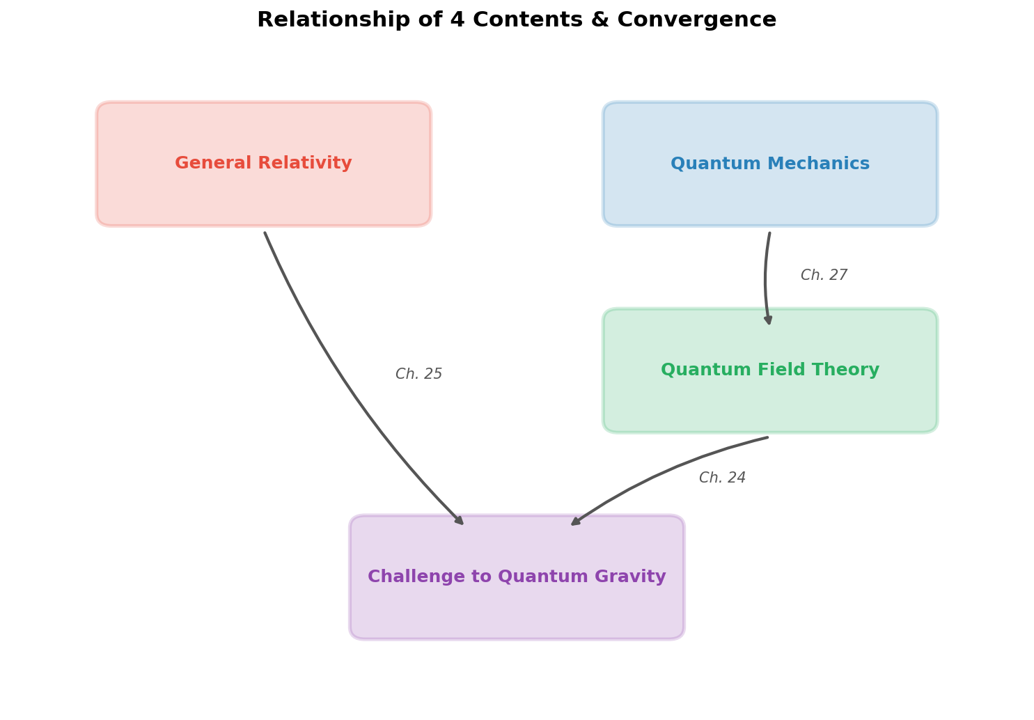
Fig. 0.3: Relationship and convergence point of the four parts. The three parts — general relativity, quantum mechanics, and quantum field theory — each converge on The Quest for Quantum Gravity, motivated by the "quantum gravity problem." QFT Ch. 24 serves as the closest entry point.

⚪ Mei: I'm curious about what that "bridge" means.

🟡 Lina: Yes, I'll touch on it in detail in a later section. As an introduction to Part VII, just keep in mind that "quantum field theory doesn't end with a string of victories — the final Part honestly surveys its own limits as well."

Summary of the Journey's Overall Map¶

🟡 Lina: Let me summarize the whole thing in one figure (Fig. 0.4 "Roadmap of all 24 chapters").

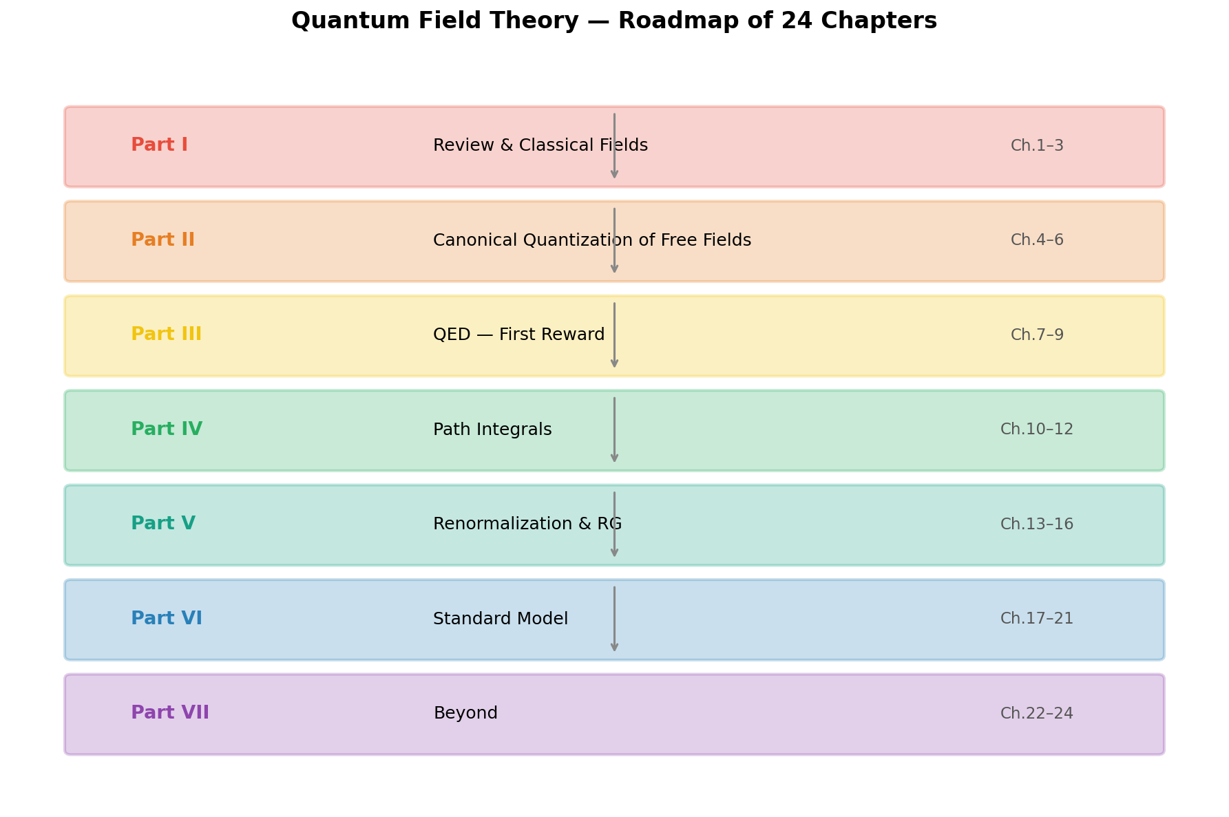
Fig. 0.4: Roadmap of all 24 chapters. The complete journey map of all 24 chapters organized into 7 Parts. Each Part builds upon the previous one.

Table 0.1: Overview of chapter structure and keywords for all 7 Parts

Part	Chapters	Theme	Keywords
I	1–3	Review and Classical Fields	Lorentz invariance, Lagrangian, Noether's theorem
II	4–6	Canonical Quantization of Free Fields	Creation/annihilation operators, anticommutation relations, gauge freedom
III	7–9	QED — The First Reward	S-matrix, Feynman diagrams, scattering cross sections
IV	10–12	Path Integrals	Feynman's sum over paths, generating functionals, Grassmann numbers
V	13–16	Renormalization	UV divergence, regularization, renormalization group, effective field theory
VI	17–21	The Standard Model	Yang-Mills, symmetry breaking, Higgs, electroweak unification, QCD
VII	22–24	Beyond	Condensed matter, non-perturbative phenomena, bridge to quantum gravity

🔵 Kai: Looking at it this way, each Part has the structure of "acquiring new tools and using them in the next Part."

🟡 Lina: Exactly. Because it's a cumulative structure, skipping ahead will cause problems later. But conversely, if you proceed step by step, you'll definitely make it to the end.

On Mathematical Tools — Introduction to the Appendices¶

🟡 Lina: In addition to the 24 chapters of the main text, I've prepared 4 Appendices.

Table 0.2: Structure and contents of the Appendices

Appendix	Contents
A	Analytical Mechanics Toolbox (functionals, field Lagrangians, canonical quantization of fields)
B	Representation Theory of the Lorentz Group
C	Gaussian Integrals and Grassmann Integrals
D	Loop Calculation Toolbox (dimensional analysis, Feynman parameters, Wick rotation)

⚪ Mei: So when new mathematical tools are needed in the main text, we just refer to the corresponding Appendix.

🟡 Lina: Right. They're designed so you can supplement the necessary mathematics without interrupting the flow of the main text. In particular, Appendix B (representations of the Lorentz group) will be referenced in Ch. 2 and Ch. 5, Appendix C (Grassmann integrals) in Ch. 12, and Appendix D (Feynman parameters, Wick rotation) in Chapters 13–14. Note that particle analytical mechanics itself — Lagrangians, Hamiltonians, Poisson brackets, the recipe for canonical quantization — is delegated to Quantum Mechanics Quantum Mechanics Appendix D, so if you haven't arrived here in the recommended reading order, please refer to that as well.

The Limits of Quantum Field Theory — Three Walls¶

🟡 Lina: Finally, let me preview what lies "beyond" this journey.

🔵 Kai: Beyond, as in after Chapter 24?

🟡 Lina: Yes. Actually, during this journey, the "limits" of quantum field theory will show their face several times. Since they're dealt with in separate chapters, they might be hard to notice individually, but when viewed together, you can see they share the same root. Let me list three.

Wall 1: Ultraviolet divergences appearing in loop calculations (Ch. 13)

🟡 Lina: When you calculate Feynman diagrams containing closed lines — loops — you need to "sum over all values (integrate)" the momentum of the particle running around the loop. If you carry out that integration to infinity, the answer diverges. Electron self-energy, photon vacuum polarization, vertex corrections — all of them give \(\infty\) when calculated straightforwardly.

🔵 Kai: Doesn't getting infinity mean "something's wrong"?

🟡 Lina: It looks that way, but no. And the next thing you learn is "renormalization" — the technique for taming infinities.

Wall 2: The existence of non-renormalizable theories (Ch. 16)

🟡 Lina: However, renormalization isn't universal. There are theories where renormalization works and theories where it doesn't. The theories where it works (QED, QCD, electroweak unification — all of the Standard Model) are called renormalizable. For example, in QED, just fitting a few physical parameters — the electron's mass and charge — to experimental values allows all remaining physical quantities — scattering probabilities, energy level shifts, \(g\)-factor corrections — to be predicted as finite values.

🔵 Kai: What does "fitting parameters to experimental values" mean?

🟡 Lina: For example, the electron's mass can't be determined by theory alone, so we input the experimentally measured value \(0.511\ \mathrm{MeV}/c^2\). Same for the charge. The "infinities" from Wall 1 can actually be absorbed by redefining (= renormalizing) these values of mass and charge. Intuitively — in the theoretical calculation, quantum corrections are added to "the electron mass without interactions" (called the "bare mass"), but those corrections turn out to be infinite. As an analogy, it's like stepping on a scale and seeing "∞ kg" displayed. But actually the zero point of the scale was off, and of the "∞ kg," the amount "∞ - 0.511 kg" was due to the zero-point offset — recalibrate the zero point and you read the correct value of \(0.511\) kg. Lumping together "bare mass + infinite correction" and reinterpreting it as "experimentally measured mass \(0.511\ \mathrm{MeV}/c^2\)" follows the same spirit. The infinity gets pushed into the difference between the "bare value" and the "observed value," disappearing from observable quantities. Once these 2 parameters (mass and charge) are fitted to experimental values, the theory calculates everything else — that's what "renormalizable" means. On the other hand, theories where infinities cannot be pushed into a finite number of parameters no matter what are called non-renormalizable.

⚪ Mei: "Can't be pushed into a finite number" means... you'd need infinitely many parameters?

🟡 Lina: Exactly. Intuitively, as you try to improve the calculation's precision — incorporating finer quantum corrections — increasing the number of loops introduces new types of divergences each time. Each time, you need to determine a new parameter experimentally. A theory that requires infinitely many parameters to be fixed by experiment to make predictions is meaningless as a physical model. And when you naively quantize gravity as a field theory — this is exactly Wall 3 — it becomes non-renormalizable.

🔵 Kai: Um... so in QED you just need to fix mass and charge, those 2 things, but for gravity you'd need infinitely many? Why is gravity alone so troublesome?

🟡 Lina: Good question. Intuitively, the coupling constant of gravity (Newton's constant \(G\)) has dimensions, and the interaction gets stronger as energy increases. So divergences get worse as you add more loops. Details in Ch. 24, but for now just remember "gravity becomes unmanageable at high energies."

Wall 3: Graviton scattering amplitudes can't be controlled (Ch. 24)

🟡 Lina: When you try to quantize gravity by introducing a spin-2 field called the graviton and applying the Feynman diagram procedure, divergences at higher loops become unmanageable. Historically, at 1-loop (one round of quantum correction) the divergence was barely avoided, but at 2-loop (two rounds of correction) it was shown to diverge conclusively (in 1986, by Goroff and Sagnotti). This means new divergences appear with each additional loop — a textbook case of "non-renormalizable."

🔵 Kai: Does that mean "handling gravity with quantum field theory is impossible"?

🟡 Lina: At the very least, it doesn't work the same way as the other forces. We'll cover this in detail in Ch. 24.

🔵 Kai: These three walls all seem to be about "infinities appearing." Is it a coincidence, or is there a common cause?

🟡 Lina: Good intuition. They actually share the same root. In quantum field theory, particles are treated as points. Points interact at a single point, causing divergences at short distances. Here, recall the correspondence "short distance = high energy" — from de Broglie's relation \(\lambda = h/p\), probing short distances requires large momentum, right? So short-distance physics is the same as high-energy physics. Since the high-energy end of the light spectrum is ultraviolet, this type of divergence is called ultraviolet divergence (UV divergence).

🔵 Kai: Ah, so that's why it's called "ultraviolet." Short wavelength = high energy = ultraviolet side.

🟡 Lina: Exactly. Wall 1's ultraviolet divergence, Wall 2's non-renormalizability, and Wall 3's difficulty of quantizing gravity — they all root in "point particles interacting at a single point."

⚪ Mei: So all three walls come from "the limits of the point-particle picture."

🔵 Kai: Because we treat them as points, it diverges at zero distance...?

🟡 Lina: Yes. This "limit of the point-particle picture" manifests most sharply as the quantum gravity problem in Ch. 24. So how do we overcome this wall? In the next section, I'll preview what lies beyond.

✅ Comprehension Check: What is the fundamental cause common to the "three walls" in quantum field theory (ultraviolet divergence, non-renormalizability, difficulty of quantizing gravity)?

Answer

In quantum field theory, particles are treated as "points (zero size)" and interactions occur at a single point. Because of this, integrals diverge at short distances (high energy = ultraviolet region). All three walls originate from this "limit of the point-particle picture."

The Bridge to Quantum Gravity — Toward The Quest for Quantum Gravity¶

🟡 Lina: So what if the fundamental objects weren't "points"? What if they were "strings" with finite extent? Interactions would occur not at a point but over a finite region, and ultraviolet divergences would be naturally softened — this is one of the motivations for string theory.

⚪ Mei: ...But is string theory the only approach to quantum gravity?

🟡 Lina: Good question. There are actually several.

String theory: Replaces point particles with 1-dimensional strings — interactions occur on "surfaces" rather than "points," softening ultraviolet divergences
Loop quantum gravity (LQG): Quantizes spacetime itself as a discrete structure — doesn't assume continuous spacetime
Asymptotic safety: Maintains the framework of quantum field theory while seeking a "fixed point" where the theory converges to finite values at high energies
Causal dynamical triangulations (CDT): Divides spacetime into small tetrahedra (4-dimensional versions of triangles) and performs path integrals over their combinations

Each of these hypotheses attempts to tackle the quantum gravity problem by rewriting somewhere among "point particles," "quantum field theory," or "classical spacetime."

🔵 Kai: Which one is correct?

🟡 Lina: At present, none have been settled by experiment. Humanity doesn't yet have experiments that can directly measure physics at the Planck scale. As shared in the Introduction — models are hypotheses. Even string theory is "one promising candidate," not "the only answer."

⚪ Mei: Then why does this site cover string theory?

🟡 Lina: Because it's the most systematically developed, and it's at a stage where much can be said both mathematically and physically. In the next journey, The Quest for Quantum Gravity Prologue, we'll pursue what that "systematization" means. String theory automatically contains the graviton and is the candidate that has been studied longest as one that avoids the renormalizability problem — in that sense, it's a "representative approach."

🔵 Kai: A representative player, but not the sole champion.

✅ Comprehension Check: The approach to the quantum gravity problem is not limited to string theory. Name two or more other approaches mentioned in the text, and state the strategy they share.

Answer

In addition to string theory, loop quantum gravity (LQG), asymptotic safety, and causal dynamical triangulations (CDT) are mentioned. What they share is a strategy of rewriting one of "point particles," "the standard methods of quantum field theory," or "classical continuous spacetime" to circumvent the wall of non-renormalizability. Note that none of these approaches has been experimentally settled at present.

🟡 Lina: Exactly. And in Chapter 24 — the final chapter of this journey — we organize how to frame the "quantum gravity problem" and send readers off to the next The Quest for Quantum Gravity Prologue. That's where the four parts truly converge. What it addresses is precisely the "quantum gravity problem" itself — structured to pair with the "quantum gravity problem" section of The Quest for Quantum Gravity Prologue.

🔵 Kai: So the philosophy of quantization learned in quantum mechanics, the geometry of spacetime learned in general relativity, and the limits of renormalization learned in quantum field theory — all of these converge into a single question?

🟡 Lina: Yes. "How should we quantize gravity?" — string theory, LQG, asymptotic safety, CDT and other hypotheses are all challenging this question. And in The Quest for Quantum Gravity, we head toward answering it. The journey through quantum field theory is also the best path for experiencing the motivation behind that quest. Experiencing the wall of renormalization in Chapters 13–16, then hitting the wall of quantum gravity in Ch. 24 — without that experience, it's hard to truly understand "why the 'Challenge of Quantum Gravity' part is necessary."

🔵 Kai: So the quantum field theory journey is also a "necessary prerequisite" for The Quest for Quantum Gravity.

🟡 Lina: Yes. That's why this journey is designed so that when you reach Ch. 24, you'll naturally feel "Ah, I see — this is why a fourth part is needed beyond here."

At the Beginning of the Journey¶

🟡 Lina: Well, the map is in hand. We'll gather the tools one by one from here. Are you ready?

🔵 Kai: ...Honestly, I'm a little scared. 24 chapters is long, and just imagining renormalization and infinities gives me a stomachache.

🟡 Lina: It'll be fine. Quantum mechanics was scary at first too, right? But you went step by step and walked through all 28 chapters. It's the same thing.

⚪ Mei: The tools we acquired in quantum mechanics — Dirac notation, commutation relations, perturbation theory, Fermi's golden rule — we worked so hard to learn them, I hope they'll be useful in the next journey.

🟡 Lina: Of course they will. They'll reappear many times throughout quantum field theory. That journey wasn't for nothing.

🔵 Kai: ...Alright. Let's go.

🟡 Lina: Then, on to Ch. 1. "Why Quantum Field Theory Is Needed" — we'll depart anew from where Quantum Mechanics Ch. 27 left off.

Next Chapter Preview¶

Ch. 1 Why Quantum Field Theory Is Needed — Continuing from Quantum Mechanics Ch. 27

We reconfirm the non-relativistic limitations of the Schrödinger equation, organize the difficulties faced by the Klein-Gordon and Dirac equations (negative energy solutions, non-positive-definite probability density), and formulate the physical reason why "particle number changing" is unavoidable as the interplay of the uncertainty principle and \(E = mc^2\), demonstrating the inevitability of the solution "quantize the field."

References¶

Schwartz, Quantum Field Theory and the Standard Model Chapter 1, "Microscopic theory of radiation"
Lancaster & Blundell, Quantum Field Theory for the Gifted Amateur Chapter 1, "The Universe as a set of harmonic oscillators"
Tong, Lectures on Quantum Field Theory Chapter 1, "Classical Field Theory" Introduction
Sakamoto Makoto, Quantum Field Theory — Focusing on Invariance and Free Fields Chapter 1, "Invitation to Quantum Field Theory"

← Ch. 28 The Quantum Gravity Pr…Ch. 1 Why Quantum Field Theor… →

Feedback on this page

Let us know if something was unclear, incorrect, or could be improved.