Chapter 7: The Metric Tensor and Introduction to the Schwarzschild Metric
Story so far: In Ch. 6, we learned about curvilinear coordinates (polar and spherical coordinates) and the mechanism of coordinate transformations using the Jacobian matrix, and introduced the metric tensor \(g_{ij}\). We confirmed that the "distance formula" changes with coordinates, but that distance itself does not depend on the choice of coordinates. However, we have not yet answered the crucial question: "How do we measure the 'distance' between two points in curved spacetime?"
Goals of this chapter
- Understand that the metric tensor \(g_{\alpha\beta}(x)\) is the "ruler" in curved spacetime, and that proper time, proper length, and light paths are all determined from this single object
- After generalizing the Minkowski metric of special relativity, present the Schwarzschild metric—which describes spacetime around a spherically symmetric star—without derivation, and "taste" gravitational time dilation and spatial stretching
- This establishes the foundation for discussing particle motion (geodesics) in subsequent chapters
Unit system in this chapter: To clarify the physical meaning of metric components, we primarily use SI units with \(c\) written explicitly. However, in places where we want concise expressions (such as reading the Schwarzschild metric), we switch to natural units \(c = 1\) or geometric units \(G = c = 1\). Such switches are indicated in the text. See Appendix D.6 for conversion rules.
7.1 Recalling "Distance" in Flat Spacetime
🟡 Lina: In the previous chapter, we learned that "coordinates just assign names to points." So what determines how "far apart" two points are?
🔵 Kai: In special relativity, it was \(ds^2 = -c^2 dt^2 + dx^2 + dy^2 + dz^2\), right?
🟡 Lina: That's right. Here, to make the structure of the metric more visible, I'll write it in units where \(c = 1\).
This is the line element of the Minkowski metric. It's the formula that gives the "squared spacetime interval" between two infinitesimally close events.
⚪ Mei: In ordinary Euclidean space, \(ds^2 = dx^2 + dy^2 + dz^2\) is just the Pythagorean theorem itself, but in spacetime the time term has a minus sign.
🟡 Lina: Exactly. That minus sign is the key that distinguishes "time" from "space." Using the Einstein summation convention we learned in Ch. 2, let's write equation (7.1) compactly.
Here \(\eta_{\alpha\beta}\) is
a \(4\times4\) matrix. This is the Minkowski metric.
🔵 Kai: In \(\eta_{\alpha\beta}\,dx^\alpha\,dx^\beta\), \(\alpha\) appears both downstairs and upstairs, and \(\beta\) appears both downstairs and upstairs, so we sum both from 0 to 3, right? The Einstein summation convention.
🟡 Lina: Right. Expanding it gives
But since the Minkowski metric is a diagonal matrix, all terms with \(\alpha \neq \beta\) vanish. What remains is
which returns us to (7.1).
⚪ Mei: So the matrix \(\eta_{\alpha\beta}\) completely determines "how to measure distance in spacetime."
✅ Comprehension Check: In the Minkowski metric line element \(ds^2 = \eta_{\alpha\beta}\,dx^\alpha\,dx^\beta\), what is the physical meaning of the minus sign on the time term?
Answer
The minus sign distinguishes "time" from "space." It causes the spacetime interval \(ds^2\) to split into three types—positive (spacelike), negative (timelike), and zero (lightlike)—thereby determining the causal structure.
7.2 The Metric Tensor—The "Ruler" for Curved Spacetime
🟡 Lina: Now we get to the main topic. In curved spacetime, a matrix that is constant everywhere like \(\eta_{\alpha\beta}\) does not exist. Instead, we use a matrix whose values change from place to place, \(g_{\alpha\beta}(x)\).
This \(g_{\alpha\beta}(x)\) is called the metric tensor, or simply the metric.
🔵 Kai: So you're saying the "markings on the ruler" change from place to place?
🟡 Lina: Good intuition. Think of the Earth's surface. Near the equator, one degree of longitude corresponds to about 111 km, but at latitude 60° north it's only about 56 km. The same "one degree of longitude" but different actual distances. That's because the metric components change with location.
⚪ Mei: Since \(\alpha\) and \(\beta\) run from 0 to 3, this is a \(4\times4\) matrix, right? Can all the components take completely different values?
🟡 Lina: Good question. There are actually constraints. In the right-hand side of \(ds^2 = g_{\alpha\beta}\,dx^\alpha\,dx^\beta\), swapping the names \(\alpha\) and \(\beta\) gives the same value, so there's no need to distinguish \(g_{\alpha\beta}\) from \(g_{\beta\alpha}\)—that is, \(g_{\alpha\beta} = g_{\beta\alpha}\) holds naturally. So it's a symmetric matrix. In addition to symmetry, the metric used in general relativity has two more important properties. First, non-degenerate—meaning the inverse matrix exists. This is equivalent to saying "the determinant is not zero" (determinants aren't covered in high school, but for a \(2\times2\) matrix \(\begin{pmatrix}a & b\\c & d\end{pmatrix}\) it's \(ad - bc\). If this is zero, the inverse matrix cannot be constructed).
🔵 Kai: If the determinant is zero, you can't make the inverse matrix... so it's like "the ruler is crushed and you can't measure distance anymore"?
🟡 Lina: Yes, good intuition. We write the components of the inverse matrix as \(g^{\alpha\beta}\) (indices written upstairs). That is, \(g^{\alpha\gamma}g_{\gamma\beta} = \delta^\alpha{}_{\beta}\) holds. Here \(\delta^\alpha{}_{\beta}\) is the Kronecker delta—a quantity that equals 1 when \(\alpha = \beta\) and 0 when \(\alpha \neq \beta\), which in matrix form is the components of the identity matrix. In other words, "metric matrix × inverse metric matrix = identity matrix." This will be needed later for the operation of "raising/lowering indices."
🔵 Kai: Symmetric, and the inverse exists. I understand so far. What's the third property?
✅ Comprehension Check: What does it mean for the metric tensor to be "non-degenerate"? And how are the components of the inverse matrix denoted?
Answer
Non-degenerate means the inverse matrix exists (the determinant is not zero). The components of the inverse matrix are written with indices upstairs as \(g^{\alpha\beta}\), satisfying \(g^{\alpha\gamma}g_{\gamma\beta} = \delta^\alpha{}_\beta\).
🔵 Kai: So indices downstairs means the metric itself, indices upstairs means the inverse matrix. The determinant isn't zero, so the inverse exists.
🟡 Lina: Right. The other property is the signature \((-,+,+,+)\). For the Minkowski metric, the diagonal components are \((-1, 1, 1, 1)\), so there's 1 minus and 3 pluses—we write this as signature \((-,+,+,+)\). A general metric isn't necessarily diagonal, but at any single point we can choose coordinates to make it diagonal—that is, make all off-diagonal components zero. This is called "diagonalization." There's a theorem in linear algebra that any real symmetric matrix can be diagonalized (this isn't covered in high school, but intuitively it means "by cleverly reorienting the coordinate axes, you can eliminate all cross terms between different directions—like \(dx\,dy\) terms—making them all zero. Imagine rotating the \(x\) and \(y\) axes in 2D to align with the principal axes of an ellipse"). This is the first step—the operation of zeroing out off-diagonal components.
As the second step, after diagonalizing, you can also make all diagonal components equal to \(+1\) or \(-1\) by rescaling each coordinate by a constant factor (scale transformation). This is a type of coordinate transformation—for example, stretching or shrinking the scale by an operation like \(x' = ax\).
🔵 Kai: Making the diagonal components \(+1\) or \(-1\)... how exactly do you do that?
🟡 Lina: For example, if a diagonal component is \(+4\), stretching the coordinate in that direction by a factor of 2 makes it \(+1\). Specifically, for \(ds^2 = 4\,dx^2\), setting \(x' = 2x\) gives \(dx = dx'/2\), so \(ds^2 = 4(dx'/2)^2 = dx'^2\). Similarly, if a diagonal component is \(-9\), with \(ds^2 = -9\,dt^2\), setting \(t' = 3t\) gives \(dt = dt'/3\), so \(ds^2 = -9(dt'/3)^2 = -dt'^2\). In general, if the diagonal component is a positive number \(a\), a scale transformation by \(\sqrt{a}\) makes it \(+1\); if it's a negative number \(-b\), scaling by \(\sqrt{b}\) makes it \(-1\). Since it's non-degenerate (determinant ≠ 0), zero never appears as a diagonal component—it's always either positive or negative.
⚪ Mei: Does the number of \(+1\)'s and \(-1\)'s remain constant regardless of the choice of coordinates?
🟡 Lina: Yes. After these two steps—(1) diagonalizing to zero out off-diagonal components, (2) scale transforming to make diagonal components \(\pm 1\)—the metric at any single point can be brought to the form \(\mathrm{diag}(\pm 1, \pm 1, \pm 1, \pm 1)\). Now, why is "the number of \(+1\)'s and \(-1\)'s constant regardless of coordinates"? Intuitively, coordinate transformations are continuous operations, so for a diagonal component to change from plus to minus, it would have to pass through zero along the way. But the determinant of a diagonal matrix is the product of all diagonal components (for \(4\times4\), the product of 4 diagonal components).
🔵 Kai: The product of all of them... for \(2\times2\), it's \(ad - bc\), and for a diagonal matrix \(b = c = 0\) so it's \(a \times d\), right?
🟡 Lina: Right. The same structure holds for \(4\times4\)—it's the product of the 4 diagonal components. So if even one diagonal component becomes zero, the determinant is also zero—contradicting non-degeneracy (determinant ≠ 0). Therefore zero cannot be crossed, and the signs cannot change (this fact is called Sylvester's law of inertia, but you don't need to remember the name).
🔵 Kai: I see—to change sign you'd have to pass through zero, but if it becomes zero then the determinant is zero, contradicting non-degeneracy, so you can't pass through... therefore the number of each sign is invariant.
🟡 Lina: Exactly. Physically speaking, even if you change coordinates, the fundamental structure of spacetime—"1 time direction and 3 space directions"—shouldn't change. The signature mathematically guarantees exactly that. For the spacetime metric, we require "one minus, three pluses." The one minus corresponds to the "time direction," and the three pluses correspond to "space directions."
⚪ Mei: To summarize, the metric tensor has three properties—symmetric, non-degenerate, and signature \((-,+,+,+)\).
Table 7.1: Three properties of the metric tensor
| Property | Meaning | Mathematical expression |
|---|---|---|
| Symmetric | Value unchanged under index exchange | \(g_{\alpha\beta} = g_{\beta\alpha}\) |
| Non-degenerate | Inverse matrix exists | \(\det(g_{\alpha\beta}) \neq 0\) |
| Signature \((-,+,+,+)\) | 1 time direction, 3 space directions | When diagonalized, 1 negative and 3 positive |
🟡 Lina: Right. Because it's symmetric, the number of independent components is reduced. Let's count. A \(4\times4\) matrix has 16 components in total, but since \(g_{\alpha\beta} = g_{\beta\alpha}\), the upper triangular part and lower triangular part have the same values—the independent ones are 4 diagonal components plus \(\frac{4\times3}{2} = 6\) components above the diagonal, totaling 10. In general, an \(n \times n\) symmetric matrix has \(\frac{n(n+1)}{2}\) independent components, and for \(n = 4\) that's \(\frac{4 \times 5}{2} = 10\). These 10 functions completely determine the geometry of spacetime—that is, the gravitational field.
🔵 Kai: 10 functions determine the gravitational field... in Newton's model it was just one potential \(\Phi\), so this is much more complex.
🟡 Lina: True. But in return, time dilation, spatial curvature, light trajectories—everything is derived from these 10 components. A single object describes everything in a unified way.
✅ Comprehension Check: How many independent components does the metric tensor \(g_{\alpha\beta}\) in 4-dimensional spacetime have? Why that number?
Answer
- Since it's a \(4 \times 4\) symmetric matrix (\(g_{\alpha\beta} = g_{\beta\alpha}\)), the number of independent components is \(4 \times 5 / 2 = 10\).
📝 Exercises:
- Reading the Minkowski metric and metric tensors → Problem B-1. Calculation of Line Element and Spacetime Classification Using the Minkowski Metric, Problem B-2. Metric Tensor and Inverse Metric of the 2-Dimensional Sphere, Problem B-6. Components and Inverse Metric of the de Sitter Type Metric, Problem M-5. Number of Independent Components of the Metric Tensor
7.3 Proper Time—The Time Ticked by "Your Own Clock"
🟡 Lina: Let's extract the most important physical quantity from the metric. Starting with proper time \(d\tau\).
🔵 Kai: Proper time is the "time ticked by a moving clock," which came up in Ch. 5, right?
🟡 Lina: Right. When a particle moves through spacetime, the time ticked by the clock carried by that particle is the proper time. Since massive particles travel slower than light, for an infinitesimal displacement along the particle's path, \(c^2 dt^2\) (the time term) is larger than \(dx^2 + dy^2 + dz^2\) (the spatial terms). Let me switch back to SI units with explicit \(c\) to discuss dimensions. The Minkowski metric is \(ds^2 = -c^2 dt^2 + dx^2 + dy^2 + dz^2\), and if the particle's speed is less than light speed, then \(c^2 dt^2 > dx^2 + dy^2 + dz^2\), so \(ds^2 < 0\)—this is a "timelike path."
🔵 Kai: \(ds^2\) becomes negative? That feels strange for something called a "square."
🟡 Lina: I understand the feeling. Think of \(ds^2\) not as "the square of something" but as the name of a single quantity called the "spacetime interval." Now, proper time \(d\tau\) is "the time ticked by a clock," so we want it to be a positive real number. That means we want \(d\tau^2\) to be positive. If \(ds^2 < 0\), then \(-ds^2 > 0\), so defining \(d\tau^2 = -ds^2\) makes it positive. However, in SI units (\(c \neq 1\)) we also need to match dimensions. The line element in SI units \(ds^2 = -c^2 dt^2 + dx^2 + dy^2 + dz^2\) has dimensions of "length squared." Meanwhile \(d\tau\) has dimensions of "time," so \(d\tau^2\) has dimensions of "time squared." Physically, in the frame where the particle is at rest (\(dx = dy = dz = 0\)), \(ds^2 = -c^2 dt^2\). In Ch. 4 we defined \(d\tau^2 = -ds^2\) in units where \(c = 1\). What happens in SI units—in Minkowski spacetime, in the frame where the particle is at rest, the coordinate clock is at rest with the particle, so coordinate time \(dt\) equals the particle's proper time \(d\tau\). Therefore \(ds^2 = -c^2 d\tau^2\), which gives
\(ds^2\) is a scalar (an invariant independent of coordinates), and \(d\tau\) is also a physical quantity independent of the choice of coordinate system—"the time ticked by the particle's own clock"—hence also a scalar. Therefore this relationship holds not just in the rest frame but in any inertial frame. The reason is that a scalar is "a quantity that has the same value regardless of which coordinate system you compute it in," so both the left side \(c^2 d\tau^2\) and the right side \(-ds^2\) don't change when you switch coordinate systems. If "left side = right side" holds in one coordinate system, then since both sides retain their values in another system, the equality continues to hold.
🔵 Kai: Ah, since both sides are scalars, proving the equality in one coordinate system means it holds in every coordinate system—that's elegant.
🟡 Lina: Right. Checking dimensions: the left side is \([\text{velocity}]^2 \times [\text{time}]^2 = [\text{length}]^2\), matching the dimension "length squared" of the right side \(-ds^2\).
From here on, I'll switch back to units with \(c = 1\). Since \(c^2 = 1\), equation (7.5) simply becomes
⚪ Mei: So \(d\tau\) is real only when \(ds^2 < 0\) (timelike interval).
🟡 Lina: Right. And for light where \(ds^2 = 0\), we get \(d\tau = 0\)—light does not experience proper time.
🟡 Lina: The proper time along a finite path is obtained by integrating along the path. Let me first explain "path parameter." When a particle moves from point A to point B in spacetime, we assign numbers to each point along the path, like \(\lambda = 0\) (departure) to \(\lambda = 1\) (arrival)—this numbering is the "parameter \(\lambda\)." The numbering is arbitrary and doesn't need to be equally spaced. Then the coordinates along the path can be written as functions of \(\lambda\): \(x^\alpha(\lambda)\). \(\frac{dx^\alpha}{d\lambda}\) is "how much coordinate \(x^\alpha\) changes when parameter \(\lambda\) changes slightly"—that is, the tangent direction component of the path.
Now, writing \(dx^\alpha = \frac{dx^\alpha}{d\lambda}\,d\lambda\) in the infinitesimal proper time \(d\tau = \sqrt{-g_{\alpha\beta}\,dx^\alpha\,dx^\beta}\)—this is just the definition of the differential, "\(\lambda\) changes by \(d\lambda\), so coordinates change by \(\frac{dx^\alpha}{d\lambda}\,d\lambda\)." Substituting gives \(d\tau = \sqrt{-g_{\alpha\beta}\,\frac{dx^\alpha}{d\lambda}\,\frac{dx^\beta}{d\lambda}}\;d\lambda\). Summing this from A to B gives
Here \(\lambda_A\) is the parameter value at the departure point and \(\lambda_B\) at the arrival point (in the example above, \(\lambda_A = 0\), \(\lambda_B = 1\)). This integral is independent of the choice of parameterization—naturally, since it's a physically measurable quantity.
🔵 Kai: Why is it independent of the parameter? The parameter is something we introduced just for convenience to write the integral, right? I understand it would be problematic if the result depended on something arbitrary, but I want to see why it really works out.
🟡 Lina: Good question. For example, if "numbering from \(\lambda = 0\) to \(1\) equally spaced" versus "numbering from \(\lambda' = 0\) to \(100\)" gave different proper times, that would be a problem—the same clock traveling the same path shouldn't give different results just because of how we number the points. So we need to verify that "the value is the same regardless of parameterization." Intuitively, it's like "changing your walking speed doesn't change the path length"—the parameter corresponds to walking speed. Below I'll confirm this with equations.
Let me first summarize what we want to show and the outline of the proof.
- What we want to show: Using a different parameter \(\lambda'\) instead of \(\lambda\) gives the same integral value (7.7)
- Proof outline: The factor \(\frac{d\lambda'}{d\lambda}\) from the chain rule and the factor \(\frac{d\lambda}{d\lambda'}\) from substitution of variables are reciprocals that cancel each other—so the integral value doesn't change
- Two steps: (i) Use the chain rule to rewrite \(\frac{dx^\alpha}{d\lambda}\), (ii) Use substitution of variables to change the integration variable to \(\lambda'\)
Step (i): Rewriting via chain rule. What does it mean to replace \(\lambda\) with a different parameter \(\lambda'\)? Each point on the path has a number \(\lambda\), but we can reassign a different number \(\lambda'\) to the same point. Then \(\lambda'\) is a function of \(\lambda\) (\(\lambda' = \lambda'(\lambda)\)), and the coordinates become the composite function \(x^\alpha(\lambda'(\lambda))\). Using the chain rule for composite functions learned in high school, \(\frac{dy}{dx} = \frac{dy}{du}\cdot\frac{du}{dx}\), with the same structure: \(\frac{dx^\alpha}{d\lambda} = \frac{dx^\alpha}{d\lambda'}\cdot\frac{d\lambda'}{d\lambda}\).
One condition is needed here—the "orientation" of the parameters must agree. That is, when \(\lambda\) increases, \(\lambda'\) also increases (\(\frac{d\lambda'}{d\lambda} > 0\)). Physically this is the natural condition of "not traversing the path backwards." Why is this necessary? When extracting \(\left(\frac{d\lambda'}{d\lambda}\right)^2\) from under the square root, \(\sqrt{a^2} = |a|\) gives an absolute value. If \(\frac{d\lambda'}{d\lambda} > 0\), then \(\left|\frac{d\lambda'}{d\lambda}\right| = \frac{d\lambda'}{d\lambda}\) and we can remove the absolute value (if it were negative, a minus sign would appear making proper time negative—physically meaningless). As a concrete check, using \(\lambda' = 2\lambda\) (so \(\lambda' = 0\) to \(2\)) instead of \(\lambda = 0\) to \(1\): \(\frac{d\lambda'}{d\lambda} = 2 > 0\) so the orientation is the same. Then \(\frac{dx^\alpha}{d\lambda} = \frac{dx^\alpha}{d\lambda'} \cdot 2\), so \(2^2 = 4\) enters under the root, and coming out gives \(2\). Meanwhile, the substitution gives \(d\lambda = \frac{1}{2}d\lambda'\), so \(2 \times \frac{1}{2} = 1\) and they cancel—the integral value doesn't change.
Under this condition, substituting the chain rule result into the integral—using \(\frac{dx^\alpha}{d\lambda} = \frac{dx^\alpha}{d\lambda'}\cdot\frac{d\lambda'}{d\lambda}\) in two places (for \(\alpha\) and \(\beta\))—\(\left(\frac{d\lambda'}{d\lambda}\right)^2\) appears under the root:
🔵 Kai: Ah, \(\frac{d\lambda'}{d\lambda}\) multiplies both \(\frac{dx^\alpha}{d\lambda}\) and \(\frac{dx^\beta}{d\lambda}\), so it becomes squared under the root. And \(\sqrt{\left(\frac{d\lambda'}{d\lambda}\right)^2} = \left|\frac{d\lambda'}{d\lambda}\right|\), but since we aligned the orientation, we can drop the absolute value and bring it out directly.
🟡 Lina: Exactly.
Step (ii): Substitution of variables. Next we want to change the integration variable from \(\lambda\) to \(\lambda'\). Substitution of variables—just like in high school when you set \(x = g(t)\) and wrote \(dx = g'(t)\,dt\)—gives \(d\lambda = \frac{d\lambda}{d\lambda'}\,d\lambda'\). Since \(\frac{d\lambda}{d\lambda'}\) is the reciprocal of \(\frac{d\lambda'}{d\lambda}\), it equals \(\frac{1}{d\lambda'/d\lambda}\). From the orientation condition (\(\frac{d\lambda'}{d\lambda} > 0\)), \(\frac{d\lambda}{d\lambda'} > 0\) as well, so the direction of integration doesn't change under substitution.
Substituting \(d\lambda = \frac{d\lambda}{d\lambda'}\,d\lambda'\) into the result of step (i), and converting the integration limits to \(\lambda' = \lambda'_A\) corresponding to \(\lambda = \lambda_A\) and \(\lambda' = \lambda'_B\) corresponding to \(\lambda = \lambda_B\):
On the right side, the factor \(\frac{d\lambda'}{d\lambda} \cdot \frac{d\lambda}{d\lambda'} = 1\) (product of reciprocals) has appeared. Since this equals 1, it vanishes:
This is the same form as the original integral written in \(\lambda'\). Therefore it's independent of the choice of parameterization.
🔵 Kai: What if you reversed the orientation—numbered in the direction of decreasing \(\lambda'\)?
🟡 Lina: Then \(\frac{d\lambda'}{d\lambda} < 0\), and when extracting from the root a minus sign appears—the result is that the integral value flips sign and "proper time becomes negative." That's physically meaningless, so we exclude it.
🔵 Kai: So the analogy the professor mentioned earlier—"changing walking speed doesn't change path length"—has been confirmed with equations. But if you change the path itself—take a different route—then the proper time does change, right?
⚪ Mei: That's right. The choice of parameterization is about "how to number the same path," but if you change the path itself, proper time changes—the twin paradox from the previous chapter was exactly that.
🟡 Lina: Exactly. When the twins reunited and their proper times differed, it was because the two traveled different paths through spacetime. It's the difference in path itself, not the parameterization, that produces the physical difference.
✅ Comprehension Check: Write the relationship between proper time \(d\tau\) and spacetime interval \(ds^2\) as an equation.
Answer
\(d\tau^2 = -ds^2\) (in units where \(c = 1\)). Proper time is defined as a real number only when \(ds^2 < 0\) (timelike interval). Light (\(ds^2 = 0\)) does not experience proper time.
7.4 Proper Length—The Distance Measured by "Your Own Ruler"
🟡 Lina: Next is proper length \(dL\). It's defined for measuring the distance between two points at a given instant—that is, for purely spatial intervals (\(ds^2 > 0\)) where the coordinate time difference is zero (\(dt = 0\)). "\(dt = 0\)" means simultaneity in the coordinate system being used. \(dt = 0\) means \(dx^0 = 0\) (since \(x^0 = t\) in units where \(c = 1\)). Then in \(ds^2 = g_{\alpha\beta}\,dx^\alpha\,dx^\beta\), all terms where \(\alpha = 0\) or \(\beta = 0\) vanish because they contain \(dx^0 = 0\) (of course \(g_{00}(dx^0)^2\) vanishes, but also "cross terms" like \(g_{0i}\,dx^0\,dx^i\)—where \(i = 1, 2, 3\) are spatial components—become zero when \(dx^0 = 0\)). What remains are only the terms where both \(\alpha, \beta\) are 1, 2, 3. That is,
Here \(i, j\) run over only the 3 spatial directions (1, 2, 3), unlike the Greek letters \(\alpha, \beta\) (0–3) (this follows the convention introduced in Ch. 4 that "Latin letters are spatial components only"). So \(g_{ij}\) is the spatial part (\(\alpha, \beta = 1, 2, 3\)) extracted from the \(4\times4\) metric tensor \(g_{\alpha\beta}\).
The finite length is similarly obtained by integration:
Here again \(i, j = 1, 2, 3\) are spatial components only (for the same reason as equation (7.8)—since \(dt = 0\), terms with \(\alpha = 0\) or \(\beta = 0\) vanish). A "path with \(dt = 0\)" means a curve that moves only through space at a fixed instant of time—imagine a line drawn in space at the moment a photograph is taken. Since there's no time-direction component, the integrand is determined by \(g_{ij}\) (the spatial-components-only metric). For a diagonal metric (where off-diagonal components are zero—the spherical coordinate metric coming up shortly is such an example), the integrand becomes \(g_{11}(dx^1/d\lambda)^2 + g_{22}(dx^2/d\lambda)^2 + g_{33}(dx^3/d\lambda)^2\). Since \(g_{11}, g_{22}, g_{33}\) are all positive, and \((dx^i/d\lambda)^2\) are squared and hence positive—the integrand is positive. For a general metric as well, the signature \((-,+,+,+)\) combined with the \(dt = 0\) condition guarantees that spatial distance is always positive. Intuitively, signature \((-,+,+,+)\) means "only the time direction is negative," so the spatial part (excluding the time direction) is all positive—meaning the spatial metric is positive definite (distance is positive in any direction). The rigorous proof involves linear algebra, so I'll skip it for now.
🔵 Kai: Proper time uses \(-ds^2\), and proper length uses \(+ds^2\). The signs are opposite.
🟡 Lina: Right. In timelike directions, \(ds^2 < 0\) so \(-ds^2 > 0\) making proper time real, and in spacelike directions, \(ds^2 > 0\) making proper length real. The metric's signature \((-,+,+,+)\) naturally provides this distinction.
🟡 Lina: Proper time is defined in the \(ds^2 < 0\) region, proper length in the \(ds^2 > 0\) region—visualizing these three regions with a light cone makes it clearer. Look at Fig. 7.1 "Three classifications of spacetime intervals and the light cone". Inside the light cone is the timelike region (where proper time is defined), outside is the spacelike region (where proper length is defined), and on the cone is lightlike. The worldline of a massive particle always passes inside the light cone—naturally, since it's slower than light.
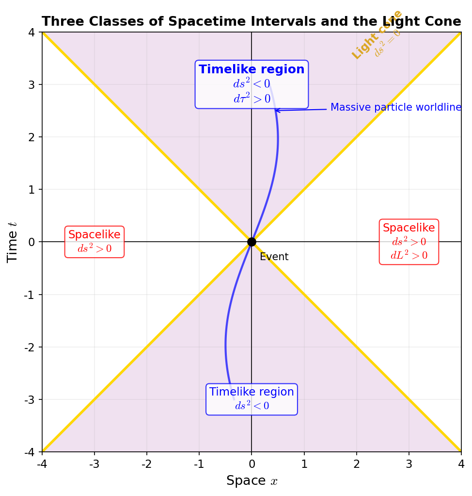
Fig. 7.1: Three classifications of spacetime intervals and the light cone. Inside the light cone is the timelike region (\(ds^2 < 0\), where proper time is defined), outside is the spacelike region (\(ds^2 > 0\), where proper length is defined), and on the light cone is lightlike (\(ds^2 = 0\)). The worldline of a massive particle always passes inside the light cone.
⚪ Mei: So in summary, once the metric tensor is given, proper time and proper length can be calculated.
🔵 Kai: For light, \(ds^2 = 0\) so proper time is zero. Then how is the path of light determined? If we can't use proper time, a different condition must be needed, right?
🟡 Lina: Good question. The path satisfying \(ds^2 = 0\) is the path light takes. Zero proper time means light always travels on the surface (\(ds^2 = 0\)) of the light cone—so the condition \(g_{\alpha\beta}\,dx^\alpha\,dx^\beta = 0\) determines the light path. Summarizing in a table:
Table 7.2: Proper time and proper length determined from the metric tensor
| Physical quantity | Definition | Condition |
|---|---|---|
| Proper time \(d\tau\) | \(d\tau^2 = -g_{\alpha\beta}\,dx^\alpha dx^\beta\) | \(ds^2 < 0\) (timelike) |
| Proper length \(dL\) | \(dL^2 = g_{ij}\,dx^i dx^j\) (\(dt = 0\)) | \(dt = 0\) (spacelike interval, \(ds^2 > 0\)) |
| Light path | \(0 = g_{\alpha\beta}\,dx^\alpha dx^\beta\) | \(ds^2 = 0\) (lightlike) |
⚪ Mei: So "which events are connected by light" is also completely determined.
🟡 Lina: Right. Knowing which events can be connected by light means knowing "which events can send signals to which other events"—that is, causal relationships are determined by the metric alone. The metric truly contains all the information about spacetime.
7.5 The Metric Works in Curvilinear Coordinates Too—Polar Coordinates in Flat Spacetime
🟡 Lina: Here's an important caveat. Just because metric components depend on position doesn't mean space is curved. To visually understand why metric components depend on position, let me discuss coordinate basis vectors. Look at Fig. 7.2 "Comparison of coordinate basis and orthonormal basis". As we learned in Ch. 6, the metric components are inner products of coordinate basis vectors: \(g_{ij} = \boldsymbol{e}_i \cdot \boldsymbol{e}_j\). So \(g_{22} = |\mathbf{e}_\theta|^2 = r^2\), meaning \(|\mathbf{e}_\theta| = r\)—the length of \(\mathbf{e}_\theta\) changes from place to place, proportional to \(r\). "The metric component \(g_{22} = r^2\) depends on position" reflects this change in basis vector length. For comparison, I've also drawn an "orthonormal basis" \(\hat{\mathbf{e}}_r, \hat{\mathbf{e}}_\theta\) that has been adjusted to have length 1 and be mutually perpendicular at every point. "Ortho" means perpendicular, "normal" means length 1.
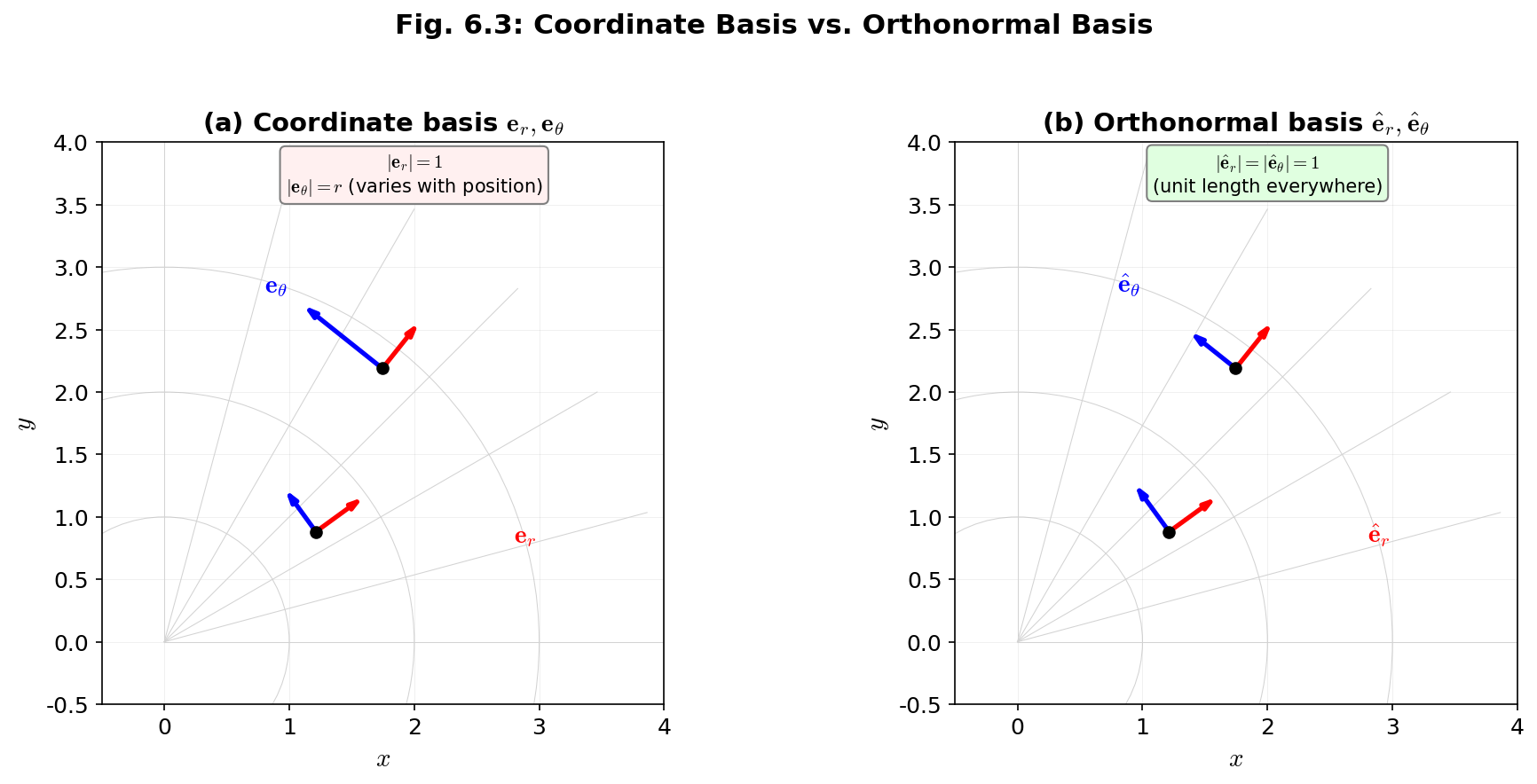
Fig. 7.2: Comparison of coordinate basis and orthonormal basis. (a) Coordinate basis \(\mathbf{e}_r, \mathbf{e}_\theta\). \(|\mathbf{e}_r| = 1\) but \(|\mathbf{e}_\theta| = r\), changing with position. (b) Orthonormal basis \(\hat{\mathbf{e}}_r, \hat{\mathbf{e}}_\theta\) has length 1 everywhere.
🟡 Lina: In part (a) of the figure, you can see the coordinate basis—\(\mathbf{e}_\theta\) changing length from place to place. That's why the metric component \(g_{22} = r^2\) depends on position. But this is due to the choice of coordinates—the space itself is flat. Part (b) shows the orthonormal basis—unlike the coordinate basis, it's normalized to length 1 at every point. This is included for visual comparison. The orthonormal basis will appear in later chapters, so just know of its existence for now.
🔵 Kai: Wait, so metric components can change even when space isn't curved?
🟡 Lina: Let's write flat spacetime in polar coordinates \((t, r, \theta, \varphi)\). The relationship to Cartesian coordinates is
🟡 Lina: Substituting into (7.1)—computing total differentials like \(dz = \cos\theta\,dr - r\sin\theta\,d\theta\) (the same procedure as in Ch. 6)—gives
🟡 Lina: Try reading off the metric components from this. Compare with \(ds^2 = g_{\alpha\beta}\,dx^\alpha\,dx^\beta\).
⚪ Mei: The coefficient of \(dt^2\) gives \(g_{00} = -1\), the coefficient of \(dr^2\) gives \(g_{11} = 1\), the coefficient of \(d\theta^2\) gives \(g_{22} = r^2\), and the coefficient of \(d\varphi^2\) gives \(g_{33} = r^2\sin^2\theta\). Summarizing:
\(g_{22} = r^2\) and \(g_{33} = r^2\sin^2\theta\) depend on position. Is this exactly the case the professor just mentioned—"components depending on position doesn't necessarily mean curvature"?
🟡 Lina: Exactly. This is due to the choice of coordinates—the spacetime itself remains flat.
🔵 Kai: So how do you determine whether something is "truly curved"?
🟡 Lina: If the Riemann curvature tensor (a quantity with four indices, constructed from second derivatives of the metric, that quantifies the degree of curvature) is non-zero, then it's truly curved. First derivatives can be eliminated by coordinate transformations, but second derivatives cannot—this is a consequence of the local flatness theorem. The specific definition and calculation will be covered in detail in later chapters; for now, just remember that "a criterion for determining curvature exists."
🟡 Lina: Let me state the local flatness theorem precisely. In any curved spacetime, at any single point, a coordinate transformation can make the metric equal to \(\eta_{\alpha\beta}\) (Minkowski metric) and simultaneously make all first derivatives of the metric zero. However, second derivatives generally cannot be made zero. Therefore the essence of "curvature" lies in the second derivatives. We'll cover this in detail in later chapters.
⚪ Mei: So even if metric components depend on position, whether that's "due to the choice of coordinates" or "true curvature" cannot be distinguished from first derivatives alone—you need to look at second derivatives to make the determination.
✅ Comprehension Check: Metric components depending on position doesn't necessarily mean space is curved. What determines whether something is "truly curved"?
Answer
If the Riemann curvature tensor, constructed from second derivatives of the metric, is non-zero, then it's truly curved. First derivatives can be eliminated by coordinate transformations, but second derivatives cannot.
7.6 Concrete Examples of the Metric as a "Ruler"
🔵 Kai: I'd like to see more concretely what it means that "the ruler markings change from place to place" when metric components depend on position.
🟡 Lina: Good question. In equation (7.11), fixing \(t, \theta, \varphi\) and changing only \(r\) by \(dr\):
The proper length in the \(r\) direction coincides directly with the coordinate change. Next, fixing \(t, r, \varphi\) and changing only \(\theta\) by \(d\theta\):
🔵 Kai: Ah, that's arc length! On a circle of radius \(r\), advancing by angle \(d\theta\) gives arc length \(r\,d\theta\). Of course!
🟡 Lina: Right. The metric component \(g_{22} = r^2\) tells us that "the actual distance per unit of coordinate \(\theta\) is \(r\) times larger." Similarly, \(g_{33} = r^2\sin^2\theta\) means "the actual distance per unit of coordinate \(\varphi\) is \(r\sin\theta\) times larger."
✅ Comprehension Check: In flat spacetime with spherical coordinates, what is the proper length when advancing by \(dr\) in the \(r\) direction? What about advancing by \(d\theta\) in the \(\theta\) direction?
Answer
In the \(r\) direction: \(dL = dr\) (since \(g_{11} = 1\), coordinate change equals proper length). In the \(\theta\) direction: \(dL = r\,d\theta\) (since \(g_{22} = r^2\), it's the arc length on a circle of radius \(r\)).
⚪ Mei: Thinking about Earth's surface: at the equator (\(\theta = \pi/2\)) the distance per degree of longitude is maximum, and approaching the pole (\(\theta = 0\)) it approaches zero as \(\sin\theta \to 0\). That's why meridian lines narrow at high latitudes in an atlas.
✅ Comprehension Check: What does the metric component \(g_{33} = r^2\sin^2\theta\) physically mean?
Answer
It means the actual distance per unit of coordinate \(\varphi\) is \(r\sin\theta\). It's maximum at the equator (\(\theta = \pi/2\)) and zero at the poles (\(\theta = 0\)).
📝 Exercises:
- Proper length in polar coordinates and metrics in curvilinear coordinates → Problem B-3. Proper Length in the \(\varphi\) Direction in Polar Coordinates, Problem M-1. Calculating the Area of a Sphere, Problem M-2. Circumference of a Circle on the Equatorial Plane
7.7 The Schwarzschild Metric—Spacetime Around a Spherically Symmetric Star
🟡 Lina: With the tools developed so far, we can now read a real "curved spacetime" metric. I'll present—without derivation—the line element for the exterior (vacuum region) of spacetime around a spherically symmetric, static mass \(M\), found by Karl Schwarzschild in 1916. Inside the star there is matter, so a different metric applies, but for the exterior alone this form works.
where
is a quantity called the Schwarzschild radius, a length scale characteristic of mass \(M\). Checking dimensions: \(G\) has dimensions \([\mathrm{m}^3\,\mathrm{kg}^{-1}\,\mathrm{s}^{-2}]\), \(M\) is \([\mathrm{kg}]\), \(c^2\) is \([\mathrm{m}^2\,\mathrm{s}^{-2}]\), so \(GM/c^2\) has dimensions \([\mathrm{m}]\)—properly a length. For the Sun, \(r_s \approx 3\,\mathrm{km}\) (extremely small compared to the Sun's radius of about 700,000 km); for Earth, \(r_s \approx 9\,\mathrm{mm}\) (extremely small compared to Earth's radius of about 6400 km). That is, for ordinary celestial bodies, the Schwarzschild radius is "buried" deep inside the body, and \(r \gg r_s\) holds in the exterior.
The unit system where \(G = 1\) is set in addition to \(c = 1\) is called geometric units. Why add \(G = 1\)? Because the combination \(GM/c^2\) appears repeatedly in the Schwarzschild metric, and being able to write it simply as \(M\) makes the formulas dramatically cleaner. Just as \(c = 1\) "unifies time and length into the same units," adding \(G = 1\) means "mass can also be measured in the same units as length." In these units, \(r_s = 2GM/c^2\) becomes \(r_s = 2M\) since \(G\) and \(c^2\) equal 1. This may look strange, but it's the same as multiplying mass by the conversion factor \(\frac{G}{c^2} \approx 7.4 \times 10^{-28}\,\mathrm{m/kg}\) in SI units to convert to length. For example, the Sun's mass \(M_\odot \approx 2.0 \times 10^{30}\,\mathrm{kg}\) gives \(GM_\odot/c^2 \approx 1.5\,\mathrm{km}\) (and \(r_s = 2 \times 1.5\,\mathrm{km} = 3\,\mathrm{km}\), matching the earlier value). In geometric units this conversion factor equals 1, so mass \(M\) directly has dimensions of length. For example, the Sun is "\(M_\odot = 1.5\,\mathrm{km}\)" (corresponding to \(GM_\odot/c^2 \approx 1.5\,\mathrm{km}\) in SI units). So \(2M/r\) is "length ÷ length," a dimensionless quantity—in SI units it would be \(2GM/(rc^2)\), also "length ÷ length" and dimensionless.
🔵 Kai: Mass having dimensions of length... being told the Sun is 1.5 km makes my brain glitch. In SI units you're multiplying by the conversion factor \(G/c^2\) to get a length, right? Setting that to 1 means the information about \(G\) and \(c\) disappears from the formulas, so it seems like it would be confusing to convert back.
🟡 Lina: That's a fair concern. But it's the same as saying in SI units "the Sun's mass, converted to length, is 1.5 km." Geometric units just set that conversion to "times 1." When converting back, you restore \(G\) and \(c\) by dimensional analysis—what we just did converting \(r_s = 2M\) back to \(r_s = 2GM/c^2\) is exactly that example. Once you get used to it, formulas become dramatically cleaner.
⚪ Mei: So the rules of geometric units are "\(c = 1\) unifies time and length, \(G = 1\) also unifies mass and length"—when you want to go back to SI, you supplement \(G\) and \(c\) by dimensional analysis.
🟡 Lina: Exactly. Writing the Schwarzschild metric in these units (\(c = 1\) so \(c^2 dt^2 \to dt^2\), \(r_s = 2GM/c^2 \to 2M\)):
🔵 Kai: Wow, it looks just like the flat spacetime (7.11), but \(dt^2\) and \(dr^2\) have \(\left(1 - \frac{2M}{r}\right)\) attached!
🟡 Lina: Right. An important note here: this \(r\) is not "the actual distance from the center." In curved space, "the distance measured straight from the center" cannot be determined from coordinates alone—you need to integrate through the metric (which we'll see in equation (7.17)). So what is \(r\)? It's a coordinate defined such that "the area of a sphere at constant \(r\) equals \(4\pi r^2\)," called the areal coordinate.
🔵 Kai: Huh, a sphere with area \(4\pi r^2\)—isn't that the same as a regular sphere? Is it worth specially defining?
🟡 Lina: In curved space, "the actual distance from center to sphere" and "the radius inferred from the area" don't coincide. As equation (7.17) will show, the actual distance in the \(r\) direction is \(dr/\sqrt{1-2M/r}\), which is longer than the coordinate difference \(dr\). So "the \(r\) where area equals \(4\pi r^2\)" and "the actual distance measured from the center" are different things—we give the name "areal coordinate" to distinguish them. Area can be calculated from just the metric on the sphere (\(g_{22}\) and \(g_{33}\)), unaffected by curvature in the \(r\) direction—because on a sphere with fixed \(r\), \(r\) doesn't change (\(dr = 0\)), so the \(g_{11}\,dr^2\) term in the line element \(ds^2\) becomes zero and vanishes. Only the \(\theta\) and \(\varphi\) terms remain.
⚪ Mei: I see—fixing \(r\) makes \(dr = 0\) so the \(r\)-direction term vanishes, meaning the geometry on the sphere is determined by \(g_{22}\) and \(g_{33}\) alone.
🟡 Lina: Right. Specifically, consider a small area element on the sphere with fixed \(r\). The proper length in the \(\theta\) direction is \(\sqrt{g_{22}}\,d\theta = r\,d\theta\), and in the \(\varphi\) direction is \(\sqrt{g_{33}}\,d\varphi = r\sin\theta\,d\varphi\). The small region bounded by these two sides is approximately rectangular (when \(d\theta\) and \(d\varphi\) are sufficiently small, the curvature of the surface is negligible). Therefore the area element is \(dA = r\,d\theta \times r\sin\theta\,d\varphi = r^2\sin\theta\,d\theta\,d\varphi\). Summing over the entire sphere gives area \(4\pi r^2\). Here a "double integral"—repeating integration twice—appears, but what it does is simple: "first move \(\varphi\) from \(0\) to \(2\pi\) to find the area of one strip, then move \(\theta\) from \(0\) to \(\pi\) to stack up the strips." Specifically, integrating over \(\varphi\) from \(0\) to \(2\pi\) gives \(\int_0^{2\pi} d\varphi = 2\pi\), then computing \(\int_0^\pi \sin\theta\,d\theta\): the antiderivative of \(\sin\theta\) is \(-\cos\theta\) (since \((\cos\theta)' = -\sin\theta\)), so \([-\cos\theta]_0^\pi = -\cos\pi -(-\cos 0) = -(-1)+1 = 2\). Multiplying everything: \(r^2 \times 2\pi \times 2 = 4\pi r^2\). In equation form: \(\int_0^\pi\int_0^{2\pi} r^2\sin\theta\,d\varphi\,d\theta = 4\pi r^2\). This follows the same approach as reading the metric on the sphere at fixed \(r\) from equation (7.11) (or the spherical coordinate line element from the previous chapter): \(ds^2 = r^2 d\theta^2 + r^2\sin^2\theta\,d\varphi^2\), and constructing the area element from the proper lengths in each direction. In the Schwarzschild metric too, the metric on the sphere has the same form (\(r^2 d\theta^2 + r^2\sin^2\theta\,d\varphi^2\)), so the area is again \(4\pi r^2\).
🔵 Kai: I see, so \(r\) isn't "distance" but "a label determined from area."
🟡 Lina: Exactly. Reading off the metric components:
⚪ Mei: The only differences from flat spacetime (7.12) are \(g_{00}\) (the time component) and \(g_{11}\) (the \(r\)-direction component). \(g_{22}\) and \(g_{33}\) have exactly the same form.
🔵 Kai: So if \(r\) becomes really large, \(\frac{2M}{r}\) is nearly zero, and it goes back to flat spacetime, right?
🟡 Lina: Exactly. Sufficiently far from the star, the gravitational influence vanishes and we recover the Minkowski metric. This is called "asymptotically flat." It's physically obvious—you shouldn't feel the gravity of a distant star. Let me summarize in a comparison table. The physical meaning in the "Difference" column will be confirmed shortly.
Table 7.3: Comparison of Schwarzschild metric and flat spacetime metric components
| Component | Flat spacetime (spherical coord.) | Schwarzschild metric | Difference |
|---|---|---|---|
| \(g_{00}\) | \(-1\) | \(-(1 - 2M/r)\) | Gravitational time dilation |
| \(g_{11}\) | \(+1\) | \((1 - 2M/r)^{-1}\) | Spatial stretching |
| \(g_{22}\) | \(r^2\) | \(r^2\) | Same |
| \(g_{33}\) | \(r^2\sin^2\theta\) | \(r^2\sin^2\theta\) | Same |
What the Schwarzschild Metric Tells Us
🟡 Lina: Several physical consequences can be read directly from this metric. Here we'll just "taste" the key points and leave detailed discussion to Ch. 9.
(1) Gravitational time dilation
🟡 Lina: Consider an observer at fixed \(r\), \(\theta\), \(\varphi\) (someone stationary around the star). Since \(dr = d\theta = d\varphi = 0\), only the \(ds^2 = g_{00}\,dt^2\) term remains in the line element. Using the proper time definition \(d\tau^2 = -ds^2\):
Therefore
This is the expression in geometric units \(c = G = 1\). To convert back to SI units, replace \(2M/r\) with \(r_s/r = 2GM/(rc^2)\), giving \(d\tau = \sqrt{1 - r_s/r}\;dt = \sqrt{1 - 2GM/(rc^2)}\;dt\).
🔵 Kai: The smaller \(r\) is (closer to the star), the smaller \(\sqrt{1 - 2M/r}\) becomes, so \(d\tau < dt\)... meaning time runs slower closer to the star!
🟡 Lina: Look at Fig. 7.3 "Gravitational time dilation". The left graph shows how the time dilation factor \(\sqrt{1 - 2M/r}\) varies with \(r\). The right image represents clocks at different positions ticking at different rates.
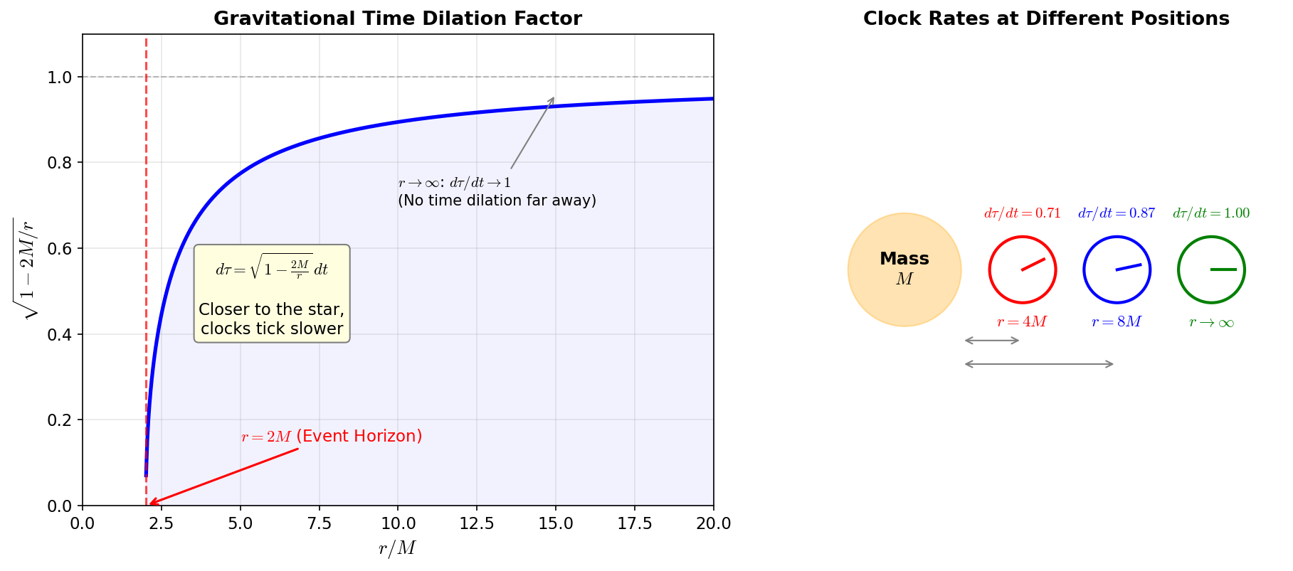
Fig. 7.3: Gravitational time dilation. Left: Graph of the time dilation factor \(\sqrt{1 - 2M/r}\). The factor reaches zero at \(r = 2M\) (event horizon) and approaches 1 at large distances (\(r \to \infty\)). Right: Clocks placed at different distances from mass \(M\). Closer to the star, clocks tick more slowly.
🟡 Lina: This is exactly the effect used in GPS satellite time corrections. The ground is closer to Earth than satellite orbits, so ground clocks run slightly slower.
🔵 Kai: GPS measures position from signal travel time, right? If the clocks drift, the position drifts too... How much correction is needed?
🟡 Lina: About 38 microseconds per day. Sounds small, but multiplied by the speed of light, that's about 11 km of drift per day. Without correction, navigation would be useless.
🔵 Kai: Just 38 microseconds causes 11 km of drift... General relativity is directly relevant to everyday technology.
⚪ Mei: At \(r = 2M\), \(g_{00} = 0\). There \(d\tau = 0\).
🔵 Kai: \(d\tau = 0\)... does that mean time stops?
🟡 Lina: More precisely, from the perspective of a distant observer, an object approaching \(r = 2M\) appears to have its time completely frozen. \(r = 2M\) is a special surface called the event horizon. We'll discuss this in detail in Ch. 16.
(2) Spatial "stretching"
🟡 Lina: Next, the proper length when advancing \(dr\) in the \(r\) direction at a given instant (\(dt = 0\)) is
🔵 Kai: Since \(1 - 2M/r < 1\), we get \(\frac{1}{\sqrt{1-2M/r}} > 1\)... so the proper length \(dL\) is longer than the coordinate difference \(dr\). Space is "stretched"!
🟡 Lina: Right. Closer to the star, the "actual distance" in the \(r\) direction is longer than what coordinates suggest. This is a concrete manifestation of "space being curved." Fig. 7.4 "Radial spatial stretching in the Schwarzschild metric" visualizes how much this "stretching" amounts to.
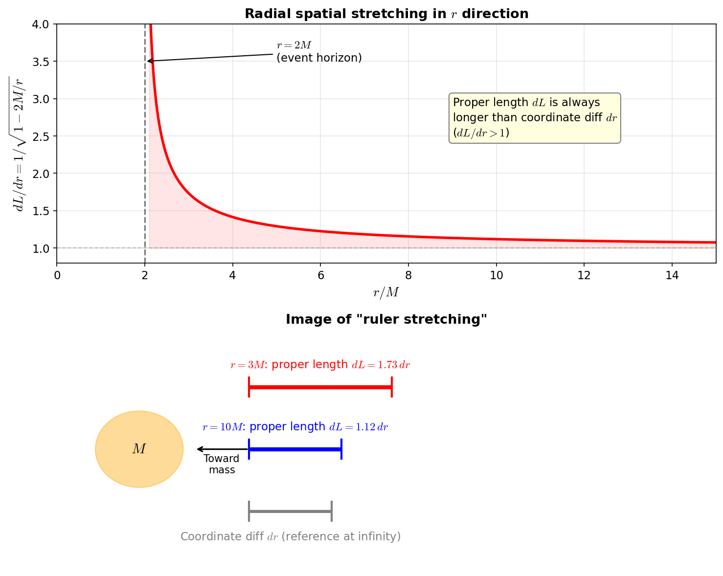
Fig. 7.4: Radial spatial stretching in the Schwarzschild metric. Top: Graph of \(dL/dr = 1/\sqrt{1 - 2M/r}\). Proper length is always longer than coordinate difference (\(dL/dr > 1\)). It diverges at the event horizon (\(r = 2M\)). Bottom: The "ruler" is stretched more at positions closer to mass \(M\).
✅ Comprehension Check: Why is the proper length \(dL\) in the \(r\) direction longer than the coordinate difference \(dr\) in the Schwarzschild metric?
Answer
Because \(dL = dr/\sqrt{1-2M/r}\) and \(1-2M/r < 1\), so \(1/\sqrt{1-2M/r} > 1\). Therefore proper length is always longer than coordinate difference. This represents the gravitational "stretching" of space.
(3) Approximation for \(r \gg 2M\)
🟡 Lina: When \(r\) is much larger than \(2M\), \(\frac{2M}{r} \ll 1\), so we can approximate \((1-2M/r)^{-1} \approx 1 + 2M/r\). This uses the formula \(\frac{1}{1-x} \approx 1 + x\) when \(|x| \ll 1\)—since \((1-x)(1+x) = 1 - x^2 \approx 1\), we get \(\frac{1}{1-x} \approx 1+x\). Then
Restoring \(c\), \(g_{00} = -(1 - 2GM/(rc^2))\), but using Newton's gravitational potential \(\Phi = -GM/r\) (Ch. 1), we get \(1 + 2\Phi/c^2 = 1 + 2(-GM/r)/c^2 = 1 - 2GM/(rc^2)\), so \(g_{00} = -(1 + 2\Phi/c^2)\). In the Schwarzschild metric, \(\Phi = -GM/r\) happens to coincide exactly with the Newtonian potential, so this is just a substitution of the definition of \(\Phi\)—no approximation is involved for \(g_{00}\). However, note that this works because the Schwarzschild metric's \(g_{00}\) happens to be linear in \(\Phi/c^2\) (of the form \(1 + 2\Phi/c^2\))—meaning you can see the correspondence with the Newtonian potential just by substituting \(\Phi\). For more complex spacetimes (e.g., around a rotating black hole), \(g_{00}\) may not be linear in \(\Phi\), so \(g_{00} = -(1+2\Phi/c^2)\) doesn't always hold exactly.
🔵 Kai: Hmm, so for \(g_{00}\) it's just substituting the Newtonian potential directly. What about \(g_{11}\)?
🟡 Lina: For \(g_{11}\), we approximate \((1-2GM/(rc^2))^{-1} \approx 1 + 2GM/(rc^2)\) (using \(r \gg r_s\)). Since \(\Phi = -GM/r\), we have \(-2\Phi/c^2 = -2(-GM/r)/c^2 = +2GM/(rc^2)\), so \(g_{11} \approx 1 - 2\Phi/c^2\). So the weak-gravity approximation enters only in \(g_{11}\). And in weak gravity, the \(g_{00}\) effect dominates, corresponding to Newton's theory. That is, Newton's model is the "weak-gravity approximation of the Schwarzschild metric." This is the mathematical content of what was previewed in Ch. 1: "Newton's model is an approximation of Einstein's model."
🔵 Kai: Wait a moment. For \(g_{00}\) it's an "exact rewriting" and only \(g_{11}\) has an "approximation"? Why does the approximation enter only on one side?
🟡 Lina: Good question. The point is the difference in mathematical form.
- \(g_{00} = -(1 - 2GM/(rc^2))\): Substituting \(\Phi = -GM/r\) gives \(-(1 + 2\Phi/c^2)\) directly. Since \(1 - 2GM/(rc^2) = 1 + 2(-GM/r)/c^2 = 1 + 2\Phi/c^2\), nothing has been discarded
- \(g_{11} = (1 - 2GM/(rc^2))^{-1}\): This has the form of a reciprocal. First approximate \(\frac{1}{1-x} \approx 1+x\) to get \(g_{11} \approx 1 + 2GM/(rc^2)\), then use \(\Phi = -GM/r\) so \(2GM/(rc^2) = -2\Phi/c^2\), giving \(g_{11} \approx 1 - 2\Phi/c^2\)
One is "direct substitution," the other is "expanding the reciprocal"—that's the reason for the asymmetry.
⚪ Mei: So the asymmetry between \(g_{00}\) and \(g_{11}\) in their relationship to \(\Phi\) comes from their different mathematical forms (one is a linear expression, the other is a reciprocal).
🔵 Kai: I see... so conversely, if \(g_{00}\) had a more complex form (say, quadratic or higher in \(r\)), the correspondence with Newtonian potential wouldn't be as clean?
🟡 Lina: Exactly. It's because the Schwarzschild metric's \(g_{00}\) happens to be linear in \(\Phi/c^2\) that it corresponds neatly to Newton's potential \(\Phi = -GM/r\). For general spacetimes it can be more complicated.
⚪ Mei: To summarize: Newton's potential appears in the \((0,0)\) component of the metric as \(g_{00} = -(1+2\Phi/c^2)\), and as the professor said, in weak gravity the time component dominates and corresponds to Newton's theory—and in the Schwarzschild metric, since \(g_{00}\) happens to be linear in \(\Phi\), this correspondence holds cleanly.
✅ Comprehension Check: In the weak-gravity approximation (\(r \gg 2M\)) of the Schwarzschild metric, how does Newton's gravitational potential \(\Phi = -GM/r\) appear in which component of the metric?
Answer
It appears in the \((0,0)\) component as \(g_{00} = -(1 + 2\Phi/c^2)\) (in the Schwarzschild metric this is an exact equality). In weak gravity, the time component dominates, corresponding to Newton's theory. Newton's model is the weak-gravity approximation of the Schwarzschild metric.
✅ Comprehension Check: In the Schwarzschild metric, what happens to time closer to the star (smaller \(r\))? Why?
Answer
Time runs slower. Proper time is \(d\tau = \sqrt{1 - 2M/r}\,dt\), and as \(r\) decreases, \(\sqrt{1 - 2M/r}\) decreases, so \(d\tau < dt\).
📝 Exercises:
- Schwarzschild metric calculations, gravitational redshift, GPS → Problem B-4. Proper Time of a Static Observer in Schwarzschild Metric, Problem B-5. Metric Components of the Schwarzschild Metric at \(r = 4M\), Problem B-7. Proper Length in the \(\varphi\) Direction in the Schwarzschild Metric, Problem M-3. Derivation of Gravitational Redshift (Complete Derivation from the Schwarzschild Metric), Problem M-4. Radial Proper Length in the Schwarzschild Metric, Problem A-1. Geometry of Constant Curvature 2-Dimensional Spaces, Problem A-2. GPS and Gravitational Redshift
Why "Without Derivation"?
🔵 Kai: But professor, where does this metric come from? It just appeared out of nowhere.
🟡 Lina: Honestly, to derive this metric requires solving the Einstein equations (Ch. 14). Since we haven't even written down those equations yet, you'll have to accept "this is the form it takes" without derivation for now. However, once the metric is given, all physical consequences—proper time, proper length, light paths—can be calculated with just the tools from this chapter. The approach is: first practice "using" the metric, then later learn how to "derive" it.
⚪ Mei: I see—even though the derivation comes later, we can extract all the physical results with our current tools.
🟡 Lina: Right. In a cooking analogy: before learning the recipe (Einstein equations), we taste the finished dish (Schwarzschild metric) to experience "what physics is in it."
7.8 Chapter Summary
🟡 Lina: Let's organize what we learned today.
- The metric tensor \(g_{\alpha\beta}(x)\) is the "ruler" in curved spacetime. It's a symmetric tensor with 10 independent components
- From the line element \(ds^2 = g_{\alpha\beta}\,dx^\alpha\,dx^\beta\), we can calculate proper time (\(d\tau^2 = -ds^2\), timelike intervals) and proper length (\(dL^2 = ds^2|_{dt=0}\), spacelike intervals)
- Even if metric components depend on position, that alone doesn't mean space is curved (it could be a coordinate effect)
- The Schwarzschild metric describes spacetime around a spherically symmetric, static mass. We "tasted" gravitational time dilation, spatial stretching, and recovery of the Newtonian potential in the weak-field limit (details in Ch. 9)
- As \(r \to \infty\) it returns to the Minkowski metric, and in the weak-gravity limit it reproduces Newton's model
🔵 Kai: We've expanded from Newton's single potential to 10 functions, but in return we get all the phenomena Newton couldn't explain—time dilation, spatial stretching, etc. But conversely, it's surprising that with 10 functions, just the condition "spherical symmetry" almost completely determines the form.
🟡 Lina: Good observation. It's precisely because symmetry imposes strong constraints that the number of independent components is drastically reduced. Why this happens will become clear after we learn the Einstein equations (Ch. 14).
🔵 Kai: Symmetry is powerful... But does just the condition "spherical symmetry" really determine it uniquely? For example, even if the star is pulsating or in the middle of exploding, would the metric be the same?
🟡 Lina: Actually, it has been proven that with just the conditions of vacuum and spherical symmetry—even if the star is pulsating—the exterior metric is uniquely the Schwarzschild metric (Birkhoff's theorem). The condition of being static isn't even needed. We'll touch on this from Ch. 14 onward.
🔵 Kai: Wow... the exterior is the same metric even with pulsation? That seems counterintuitive. Why doesn't internal variation affect the outside?
🟡 Lina: Actually, a similar phenomenon exists in Newtonian gravity. Outside a spherically symmetric mass distribution, the gravitational field is the same as if all the mass were concentrated at the center—Newton's shell theorem. Birkhoff's theorem can be thought of as the general relativistic version. Spherical symmetry imposes such a strong constraint that it "prevents information from leaking out."
🔵 Kai: I see. And one more thing I was wondering—in this chapter I understood that the metric is a "ruler" and we can read off time dilation and spatial stretching. But how particles move must be determined separately, right? How do you even define "going straight" in curved spacetime? If it's curved, "straight" doesn't seem to exist...
🟡 Lina: That's exactly the topic of the next chapter. I'll give you a hint: if you have a "ruler," you can measure the "length" of a path—and you use a principle that selects "the most efficient path." "Straight" in curved spacetime—the geodesic—is defined this way.
🔵 Kai: "The most efficient path"... is that like the principle of least action from Ch. 1? But minimizing versus maximizing the action are different, right? Do we maximize or minimize proper time...?
🟡 Lina: Great question. Whether it's "minimum" or "maximum"—the answer and reasoning will be carefully worked through in the next chapter. Look forward to it.
⚪ Mei: In this chapter we went from "ruler" (metric) → "how to measure time and distance" (proper time, proper length) → "concrete example" (Schwarzschild metric), so next comes "how to move in that spacetime"—geodesics—which is a logically natural progression.
Preview of the Next Chapter
We now know that the metric provides the "ruler" for spacetime. But what does it mean for a particle to "go straight" in that curved spacetime? In Ch. 8, we derive the geodesic equation as the path that extremizes proper time. The motion of a freely falling particle is described by this equation, replacing Newton's equation of motion—the "model of motion" in general relativity finally reveals itself.
References
- Hartle, J. B. (2003). Gravity: An Introduction to Einstein's General Relativity, Chapter 7. Addison-Wesley.
- Schutz, B. F. (2022). A First Course in General Relativity, 3rd ed., Chapter 7. Cambridge University Press.
- Tong, D. (2019). General Relativity (Cambridge lecture notes), Chapter 6.
- Lancaster, T. & Blundell, S. J. (2014). General Relativity for the Gifted Amateur, Chapter 3.
- Ishii, T. (2013). Understanding General Relativity Step by Step with Equations, Chapter 7: "General Relativity." Beret Publishing.
Feedback on this page
Let us know if something was unclear, incorrect, or could be improved.