Chapter 2: The Duality of Light and Matter — de Broglie Waves and Experimental Confirmation
Story so far:
In Ch. 1, we saw three crises that classical physics faced—black-body radiation, the photoelectric effect, and atomic stability. Through Planck's quantum hypothesis \(E = h\nu\) and Einstein's light quantum hypothesis, the revolutionary picture emerged that light is "both a wave and a particle simultaneously." It was established that a photon's energy is \(E = h\nu\). In this chapter, we first confirm that since photons are massless particles, \(E = pc\) holds and \(p = h/\lambda\) follows. We then see how Compton scattering experimentally confirmed the photon's momentum, before proceeding to de Broglie's matter wave hypothesis.
Goals of this chapter
- Extend the "coexistence of particle and wave nature" that began with light to matter particles
- Motivate de Broglie's matter wave hypothesis \(\lambda = h/p\), trace its experimental confirmation through the Davisson-Germer experiment and electron diffraction, and make clear that a "unified description of particles and waves" is necessary
- Furthermore, show that de Broglie's relation is the root of the uncertainty principle, and that it is the key to explaining atomic stability
- Through this, appreciate the need for a new framework that transcends the classical "wave or particle" dichotomy
2.1 Compton Scattering — Is the Photon's Momentum "Real"?
🟡 Lina: In the previous chapter, we derived the photon energy \(E = h\nu\) from Einstein's light quantum hypothesis. Now let's think about the photon's momentum. A photon is a massless particle. The energy-momentum relation for a massless particle is \(E = pc\)—we'll confirm this later by substituting \(m = 0\) into the special relativity formula \(E^2 = (pc)^2 + (mc^2)^2\). But actually, you can get the same result just by combining \(E = h\nu\) with the basic wave relation \(c = \lambda\nu\) (speed of light = wavelength × frequency). \(p = E/c = h\nu/c = h\nu/(\lambda\nu) = h/\lambda\). So the photon's momentum is \(p = h/\lambda\). But there's something I want to confirm here. If a photon has momentum, it should transfer that momentum when it hits something, right?
🔵 Kai: Like when billiard balls collide?
🟡 Lina: Exactly that image. If light truly behaves as a particle with momentum \(p = h/\lambda\), then when you shoot light at an electron, it should scatter according to the conservation laws of energy and momentum. The person who experimentally confirmed this was Compton. It was in 1923. In other words, while the photoelectric effect showed that "the photon's energy is real," Compton scattering shows that "the photon's momentum is also real."
⚪ Mei: I see—the reality of energy and the reality of momentum were confirmed by separate experiments.
🟡 Lina: Exactly. Let me explain the experimental setup.
Experimental Setup
🟡 Lina: X-rays (light with wavelength \(\lambda\)) are directed at a stationary electron. The wavelength \(\lambda'\) of the scattered X-ray is measured. In classical wave theory, the wavelength shouldn't change before and after scattering—the wave just shakes the electron, which re-radiates at the same frequency.
🔵 Kai: But in the experiment, it did change?
🟡 Lina: It changed. Moreover, the amount of wavelength change varied systematically with the scattering angle \(\theta\) (the angle by which the X-ray was deflected). This can be naturally explained by thinking of "light colliding with an electron as a particle." Take a look at Fig. 2.1 "Schematic diagram of Compton scattering".
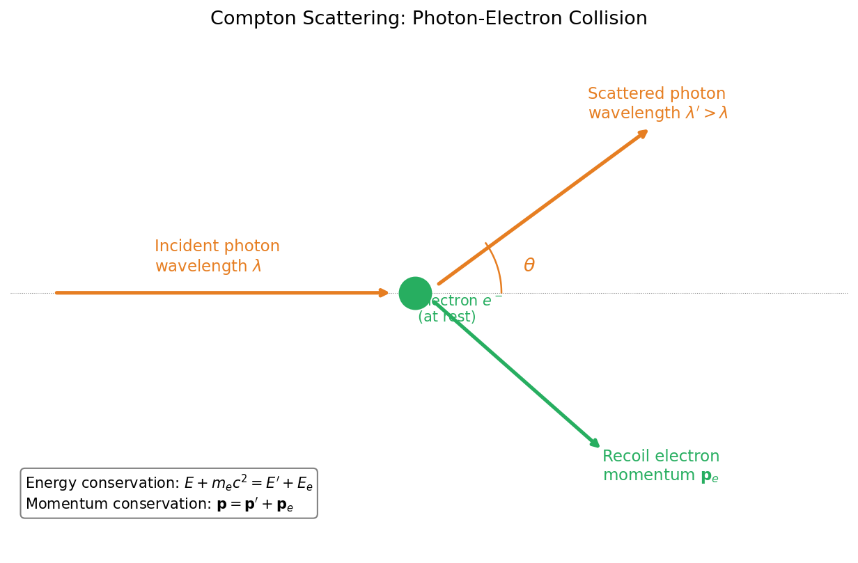
Fig. 2.1: Schematic diagram of Compton scattering. A photon with wavelength \(\lambda\) collides with a stationary electron, producing a scattered photon (wavelength \(\lambda' > \lambda\)) and a recoil electron. The relationship between the scattering angle \(\theta\) and the wavelength change is determined by the conservation of energy and momentum.
Derivation from Momentum Conservation
🟡 Lina: Let's treat the photon as a particle with momentum \(p = h/\lambda\) and write down energy conservation and momentum conservation. Let the incident photon's momentum be \(\mathbf{p}\), the scattered photon's momentum be \(\mathbf{p}'\), and the recoil electron's momentum be \(\mathbf{p}_e\). 🟡 Lina: First, energy conservation. Here we need to use a result from special relativity. The reason is that the X-ray photon's energy can be a non-negligible fraction of the electron's rest energy \(m_e c^2 \approx 0.511\) MeV (tens of keV, meaning several percent or more of the rest energy), so the recoil electron can be accelerated to considerable speeds. For such high-speed particles, the high school formula \(E = \frac{1}{2}mv^2\) becomes inaccurate. The correct expression, according to special relativity, for the energy of a particle with mass \(m\) and momentum \(p\) is
This is a formula derived from Einstein's special relativity, expressing the idea that "even at rest, a particle has energy \(mc^2\) corresponding to its mass, and when moving, additional energy corresponding to momentum \(p\) is added"—in a form resembling the Pythagorean theorem. The derivation belongs to special relativity, so for now please accept it as "the correct result."
🔵 Kai: Like the Pythagorean theorem—the hypotenuse of a right triangle is the total energy, and the two sides are \(pc\) and \(mc^2\)?
🟡 Lina: Yes, that's a great image. If you substitute zero mass (\(m = 0\)), you get \(E = pc\)—the fundamental relation connecting a photon's energy and momentum. So this formula is a general relation that holds for all particles, including photons. By the way, when a particle's speed is much less than the speed of light (\(p \ll mc\)), \((pc)^2\) is small compared to \((mc^2)^2\), so factoring \((mc^2)^2\) from \(E^2 = (mc^2)^2 + (pc)^2\) gives \(E = mc^2\sqrt{1 + (p/(mc))^2}\). Setting \(x = (p/(mc))^2 \ll 1\) and using the approximation \(\sqrt{1+x} \approx 1 + x/2\), we get \(E \approx mc^2\bigl(1 + \frac{1}{2}(p/(mc))^2\bigr) = mc^2 + \frac{p^2}{2m}\). At low speeds \(p \approx mv\), so substituting gives \(E \approx mc^2 + \frac{1}{2}mv^2\) (rest energy + kinetic energy), which is consistent with high school physics. The approximation \(\sqrt{1+x} \approx 1 + x/2\) (when \(x \ll 1\)) used here is a tangent line approximation. This comes from the concept of differentiation taught in high school math. Since the slope of \(f(x) = \sqrt{1+x}\) at \(x = 0\) is \(f'(0) = 1/2\), when \(x\) is small we can approximate \(f(x) \approx f(0) + f'(0) \cdot x = 1 + x/2\) with a straight line—a tangent line approximation. For example, if \(x = 0.01\), then \(\sqrt{1.01} = 1.00499\ldots\), and \(1 + 0.01/2 = 1.005\) is nearly identical. When \(x\) is sufficiently small, higher-order terms (\(x^2\) and above) can be neglected.
⚪ Mei: At high speeds we use the relativistic formula, and at low speeds it reduces to high school physics—they connect properly.
🟡 Lina: Exactly. For photons, mass is zero so \(E = pc\). And since \(p = h/\lambda\), we get \(E = hc/\lambda\) (you get the same result by combining \(E = h\nu\) with the basic wave relation \(c = \lambda\nu\) (speed of light = wavelength × frequency)). For the electron, which has mass \(m_e\), we use \(E_e^2 = (p_e c)^2 + (m_e c^2)^2\). Also, the energy of a stationary electron (\(p = 0\)) is found by substituting \(p = 0\) into this formula: \(E = m_e c^2\). This is Einstein's famous \(E = mc^2\), the relativistic consequence that mass itself possesses energy.
🔵 Kai: Having energy even when not moving... that's strange...
🟡 Lina: It goes against everyday intuition, but in relativity this is correct—mass is a form of energy. A stationary electron "possesses" energy \(m_e c^2\). So the total energy before the collision must include not just the incident photon's energy, but also the stationary electron's \(m_e c^2\). Let me write down the conservation laws.
Let me define the symbols here. \(E_e\) and \(p_e\) are the energy and momentum of the recoil electron, and \(\phi\) is the recoil angle of the electron (the angle between the incident direction and the electron's scattering direction). Check the configuration in Fig. 2.1 "Schematic diagram of Compton scattering".
Energy conservation (the left side is the sum of the incident photon's energy \(hc/\lambda\) and the stationary electron's rest energy \(m_e c^2\); the right side is the sum of the scattered photon's and recoil electron's energies):
\(x\)-direction momentum conservation (taking the incident direction as the \(x\)-axis):
\(y\)-direction momentum conservation (with the scattered photon going to the \(+y\) side and the recoil electron to the \(-y\) side):
For the electron, the relativistic relation \(E_e^2 = (p_e c)^2 + (m_e c^2)^2\) holds.
By eliminating \(E_e\), \(p_e\), and \(\phi\) (the electron-related quantities) from these three equations, we obtain a relation involving only the incident and scattered photon wavelengths and the scattering angle. The strategy is: from the \(y\)-direction equation get \(p_e\sin\phi = (h/\lambda')\sin\theta\); rearrange the \(x\)-direction equation to get \(p_e\cos\phi = h/\lambda - (h/\lambda')\cos\theta\); square both and add them, using \(\sin^2\phi + \cos^2\phi = 1\) to eliminate \(\phi\), yielding an equation in \(p_e^2\) alone. Then express \(E_e\) in terms of \(\lambda\), \(\lambda'\) from energy conservation, substitute into the relativistic relation \(E_e^2 = (p_e c)^2 + (m_e c^2)^2\) to eliminate \(p_e\) as well—the calculation is somewhat lengthy, but the result takes a clean form:
The detailed elimination procedure can be verified in the practice problem (Problem B-2. In the Compton scattering formula (2.1), find the wavelength shift for scattering angle).
Here: - \(\lambda\): wavelength of the incident X-ray - \(\lambda'\): wavelength of the scattered X-ray - \(m_e\): electron mass (\(9.109 \times 10^{-31}\) kg) - \(\theta\): scattering angle (angle between incident and scattered directions) - \(h/(m_e c)\): a constant called the Compton wavelength
🔵 Kai: How large is \(h/(m_e c)\)?
🟡 Lina: Let's calculate it.
About 0.024 Å (angstroms). Since the X-rays Compton used had a wavelength of about 0.7 Å, this is a change of several percent—easily measurable.
⚪ Mei: Looking at equation (2.1), if \(\theta = 0\) (forward scattering) then \(\lambda' = \lambda\) and the wavelength doesn't change. If \(\theta = 180°\) (backscattering), the wavelength shift is maximum at \(2h/(m_e c)\).
🟡 Lina: Perfect. And Compton's experimental results agreed beautifully with the prediction of equation (2.1). Fig. 2.2 "Compton scattering wavelength shift \(\Delta\lambda = \lambda_C(1-\cos\theta)\) shown as a function of scattering angle \(\theta\)" shows the relationship between wavelength change and scattering angle.
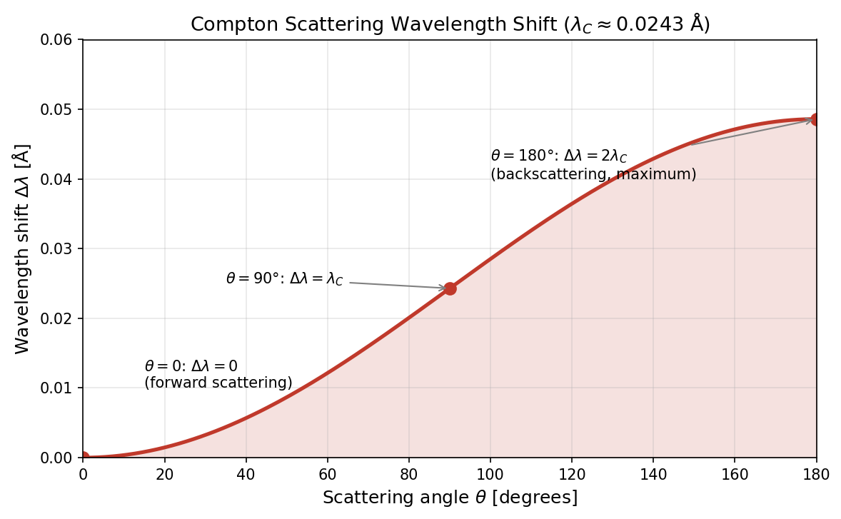
Fig. 2.2: Compton scattering wavelength shift \(\Delta\lambda = \lambda_C(1-\cos\theta)\) shown as a function of scattering angle \(\theta\). It is zero at \(\theta = 0\) and reaches its maximum value \(2\lambda_C\) at \(\theta = 180°\). \(\lambda_C = h/(m_e c) \approx 0.0243\) Å is the Compton wavelength.
What Compton Scattering Demonstrates
🟡 Lina: What makes this experiment decisively important is the following:
- The photon collides with the electron as a "particle" with momentum \(p = h/\lambda\)
- Energy and momentum are conserved before and after the collision
- Classical wave theory (Thomson scattering—a model where the electron re-radiates at the same frequency as the incident wave) cannot explain the wavelength change
In other words, the photon's momentum is not a "computational convenience" but a physically real quantity verifiable by experiment.
🔵 Kai: So there's no longer any doubt that light is a particle. But in interference experiments, it behaves as a wave, right? If both experimental results are correct...
🟡 Lina: Yes, both are correct. In interference and diffraction experiments, light definitely behaves as a wave, and in Compton scattering, it definitely behaves as a particle. It seems contradictory, but neither experimental fact can be overturned. So light is not "wave or particle" but something that possesses both properties. Accepting this situation, let's move forward.
🔵 Kai: Both a wave and a particle... but waves and particles are opposite things, aren't they? Waves spread out, and particles exist at a point. How can the same thing be both?
🟡 Lina: That question strikes right at the heart of the matter. We can't fully answer it yet, but we'll reveal it step by step in the latter half of this chapter and the next chapter. At this stage, just keep in mind that "the binary choice of wave or particle cannot capture the full picture."
🔵 Kai: Hmm, it's unsatisfying, but... I'll carry this discomfort forward. If it's "neither a wave nor a particle," then how exactly do we describe it...?
🟡 Lina: The answer to that question is precisely "quantum mechanics" itself, which we'll construct in the coming chapters. Let's start by clarifying "what is behaving as a wave" in the next section.
✅ Comprehension Check: Why can't Compton scattering be explained by classical wave theory (Thomson scattering)?
Answer
In classical wave theory, the electron re-radiates at the same frequency as the incident wave, so the wavelength doesn't change before and after scattering. However, experiments observed a wavelength change that depends on the scattering angle. This can only be explained by considering photons as particles with momentum \(p = h/\lambda\) that collide with electrons following the conservation laws of energy and momentum.
✅ Comprehension Check: In Compton scattering, what is the wavelength change \(\Delta\lambda = \lambda' - \lambda\) when the scattering angle is \(\theta = 90°\)?
Answer
Setting \(\theta = 90°\) in equation (2.1), \(\cos 90° = 0\), so \(\Delta\lambda = h/(m_e c) \approx 2.43 \times 10^{-12}\) m. This equals the Compton wavelength itself.
📝 Exercises:
- Calculation of Compton scattering wavelength shift → Problem B-2. In the Compton scattering formula (2.1), find the wavelength shift for scattering angle
2.2 de Broglie's Matter Wave Hypothesis — A Reversal of Thinking
🟡 Lina: So far, we've learned the following about light:
Table 2.1: Physical quantities corresponding to the wave and particle nature of light
| Property of light | Corresponding physical quantities |
|---|---|
| Wave nature | Wavelength \(\lambda\), frequency \(\nu\) |
| Particle nature | Momentum \(p\), energy \(E\) |
And the relations connecting them are:
🔵 Kai: These are the equations from Ch. 1.
🟡 Lina: Yes. Then in 1924, the French physicist de Broglie made a bold proposal in his doctoral thesis. His question was this:
"Light was thought to be a wave, but it actually has particle properties too. Then conversely—might matter particles actually have wave properties as well?"
🔵 Kai: A reversal of thinking! But I can sort of understand why photons behave as waves since they have no mass—but for electrons or balls that have mass, what does it concretely mean to "have a wavelength"? What is waving?
🟡 Lina: That's a very good question. "What is waving" will be addressed in the second half of this chapter ("What Is "Behaving as a Wave"?"). For now, let's first look at what hypothesis de Broglie proposed, and then think about its meaning.
🔵 Kai: I'm curious, but... okay, please make sure to come back to it later.
🟡 Lina: I promise. Now, de Broglie hypothesized that equations (2.3) and (2.4) hold not just for light but for all matter particles. That is, a particle moving with mass \(m\) and velocity \(v\) has a corresponding wavelength:
This is called the de Broglie wavelength. In general, \(\lambda = h/p\) is the basic form, and one may use relativistic momentum for \(p\). However, writing \(p = mv\) here is an approximation valid when the particle's speed is much less than the speed of light. In Compton scattering, the electron reaches high speeds requiring relativistic momentum, but for the examples we'll treat next (electrons accelerated through voltages of a few hundred volts), \(p = mv\) is sufficiently accurate.
⚪ Mei: It's just solving equation (2.4) for \(\lambda\). But extending a relation that held for photons to electrons and balls is quite bold.
🟡 Lina: Indeed. The review committee at the time was perplexed. De Broglie's advisor Langevin sent the thesis to Einstein for his opinion. Einstein commented that "this has lifted a corner of a great veil."
Why This Hypothesis Is Natural
🟡 Lina: Let me explain in more detail the motivation that led de Broglie to this hypothesis. He was well-versed in special relativity and reasoned as follows.
The relations that hold for photons: - Connecting energy \(E\) and frequency \(\nu\): \(E = h\nu\) - Connecting momentum \(p\) and wavelength \(\lambda\): \(p = h/\lambda\)
These have a natural form within relativity. In special relativity, energy and the three components of momentum (\(p_x, p_y, p_z\)) form an inseparable set that combines into a single quantity. This is called the 4-momentum—"4" because there are 4 components total: the time direction (energy) + 3 spatial directions (momentum). Similarly, the frequency \(\nu\) and the reciprocals of wavelength (\(1/\lambda_x, 1/\lambda_y, 1/\lambda_z\)) also form a set as a single quantity (the 4-wavevector). The key point is that when you look at \(E = h\nu\) and \(p = h/\lambda\) together, they become a single proportionality relation: "4-momentum = \(h\) × 4-wavevector." In other words, the relations connecting the particle and wave properties of photons are not two separate equations within the relativistic framework, but are unified as one natural relation. And since the principles of relativity apply equally to all objects, not just photons, there's no reason to restrict this relation to photons alone—that was de Broglie's insight.
🔵 Kai: 4-momentum and 4-wavevector... honestly I don't quite get it yet... but basically, because the form is "elegant" relativistically, it should hold for matter too? But is "elegant therefore correct" really enough to believe it?
🟡 Lina: Right. "4-" means "a set of 4 components: 1 time direction + 3 spatial directions," and in relativity, since time and space cannot be treated separately, such sets naturally appear. But the details can wait until you properly study relativity. What I want you to take away at this stage is just one point: \(E = h\nu\) and \(p = h/\lambda\) are not two equations that happen to sit side by side, but combine into one natural relation within relativity. It's similar to how "electric fields and magnetic fields appear to be separate phenomena, but are actually two aspects of a single thing called the electromagnetic field"—in high school you learn about electric and magnetic fields separately, but in Maxwell's theory they unite as one "electromagnetic field." De Broglie believed in "the symmetry of nature." If light has both wave and particle nature, then matter should have the same symmetry. This was an unsubstantiated hypothesis at the time, but it would soon be confirmed by experiment.
✅ Comprehension Check: Explain the motivation that led de Broglie to his matter wave hypothesis from the perspective of special relativity.
Answer
In special relativity, energy and momentum form a set as the 4-momentum, and frequency and the reciprocal of wavelength form a set as the 4-wavevector. The relations \(E = h\nu\) and \(p = h/\lambda\) that hold for photons represent a relativistically natural relationship where these two sets are proportional. De Broglie considered that this symmetry should hold for matter particles as well.
Notation Using Angular Frequency and Wavenumber
🟡 Lina: In physics, it's common to use the angular frequency \(\omega = 2\pi\nu\) (phase change per second measured in radians) rather than frequency \(\nu\), and the wavenumber \(k = 2\pi/\lambda\) (phase change per unit length measured in radians) rather than wavelength \(\lambda\). This way, \(2\pi\) doesn't appear explicitly in formulas, and rewriting with \(\hbar = h/(2\pi)\):
This is cleaner, and we'll frequently use this form in later chapters.
🔵 Kai: What's the point of changing notation? Can't we just stick with \(h\) and \(\nu\)?
🟡 Lina: When writing wave equations, the phase always comes with \(2\pi\) as in \(2\pi\nu t - 2\pi x/\lambda\). Using \(\omega\) and \(k\), the phase is simply \(\omega t - kx\). This simplicity will matter when we deal with wave equations later.
⚪ Mei: The relationship between \(h\) and \(\hbar\) is \(\hbar = h/(2\pi)\), so numerically \(\hbar \approx 6.626 \times 10^{-34} / (2\pi) \approx 1.055 \times 10^{-34}\) J·s. Equations (2.3)–(2.4) and equations (2.6)–(2.7) express the same content, just differing in how the \(2\pi\) factor is handled.
🟡 Lina: Exactly. Equations (2.5)–(2.7) are sometimes collectively called the Einstein-de Broglie relations.
✅ Comprehension Check: In the notation \(E = \hbar\omega\), \(p = \hbar k\) using \(\hbar\), what do \(\omega\) and \(k\) respectively represent?
Answer
\(\omega = 2\pi\nu\) is the angular frequency, measuring phase change per second in radians. \(k = 2\pi/\lambda\) is the wavenumber, measuring phase change per unit length in radians. By using \(\hbar = h/(2\pi)\) instead of \(h\), the \(2\pi\) factors disappear from the formulas, giving a cleaner form.
✅ Comprehension Check: State the core of de Broglie's matter wave hypothesis in one sentence.
Answer
Every matter particle with momentum \(p\) has a corresponding wave with wavelength \(\lambda = h/p\). This extends the relation \(p = h/\lambda\), which holds for photons, to matter particles such as electrons.
2.3 Calculating Matter Wave Wavelengths — Why We Don't See Them in Daily Life
🟡 Lina: Let's use the de Broglie wavelength formula \(\lambda = h/(mv)\) to calculate some specific values. First, recall how small \(h\) is:
This value is incredibly tiny. So when the denominator \(mv\) has an everyday magnitude, \(\lambda\) becomes unimaginably short.
Example 1: A Baseball
🟡 Lina: The de Broglie wavelength of a baseball with mass \(m = 0.15\) kg and velocity \(v = 40\) m/s is:
🔵 Kai: \(10^{-34}\) m!? The size of an atomic nucleus is \(10^{-15}\) m, so this is \(10^{19}\) times smaller than that...
🟡 Lina: Exactly. There's no way to detect such a wavelength. That's why wave behavior is unobservable for everyday objects.
Example 2: An Electron
🟡 Lina: Next, let's consider an electron (mass \(m_e = 9.109 \times 10^{-31}\) kg) accelerated through 100 V. At around 100 V, the electron's speed is below a few percent of the speed of light, so the non-relativistic \(p = mv\) is sufficiently accurate. When an electron is accelerated through voltage \(V_{\mathrm{acc}}\), the kinetic energy gained is:
Here \(e = 1.602 \times 10^{-19}\) C is the elementary charge. Solving for velocity:
This is about 2% of the speed of light (\(3.0 \times 10^8\) m/s), so the non-relativistic \(p = mv\) is sufficiently accurate. Therefore the de Broglie wavelength is:
⚪ Mei: \(1.23 \times 10^{-10}\) m... that's 1.23 Å, which is roughly the same order as atomic spacings!
🟡 Lina: That's the key point. For wave diffraction to occur, you need a "grating" of comparable size to the wavelength. Crystal atomic spacings are a few Å, which matches the electron's de Broglie wavelength perfectly. Compare the wavelengths of various particles in Fig. 2.3 "Comparison of de Broglie wavelength \(\lambda = h/p\) (logarithmic scale). The baseball's wavelength is \(10^{-34}\) m"—you can see at a glance how incredibly small the baseball's \(10^{-34}\) m is. By the way, if you increase the accelerating voltage further, the wavelength becomes even shorter. An optical microscope cannot resolve anything finer than the wavelength of visible light (hundreds of nm), but if you accelerate electrons through tens of thousands of volts, the wavelength drops below 0.01 nm, making atomic-level structures "visible"—this is the principle behind the high resolution of electron microscopes.
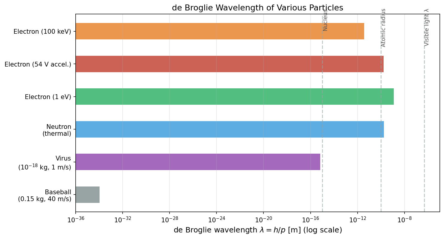
Fig. 2.3: Comparison of de Broglie wavelength \(\lambda = h/p\) (logarithmic scale). The baseball's wavelength is \(10^{-34}\) m—undetectable. Accelerated electrons have wavelengths comparable to atomic spacings (Å) and can be observed as crystal diffraction. High-energy electrons have even shorter wavelengths, forming the basis for the high resolution of electron microscopes.
🔵 Kai: So if we shoot electrons at a crystal, diffraction might occur! ...But electrons are particles, right? Can particles really diffract?
🟡 Lina: The people who experimentally confirmed this were Davisson and Germer. To give you the conclusion: it really does happen.
✅ Comprehension Check: Explain why the de Broglie wavelengths of a baseball and an accelerated electron differ so greatly, based on the formula \(\lambda = h/(mv)\).
Answer
Since Planck's constant \(h \approx 6.6 \times 10^{-34}\) J·s is extremely small, when the denominator momentum \(mv\) has an everyday magnitude (baseball: \(mv \sim 6\) kg·m/s), the wavelength is \(10^{-34}\) m—undetectably short. On the other hand, the electron's mass is extremely small at \(10^{-30}\) kg, so even at moderate speeds its momentum is small enough that the wavelength reaches the order of atomic spacings (Å), making it observable as diffraction.
Convenient Formula Relating Accelerating Voltage and de Broglie Wavelength
🟡 Lina: For electrons, combining equations (2.9) and (2.10) gives a convenient formula. Since \(p = m_e v = \sqrt{2m_e eV_{\mathrm{acc}}}\):
Looking at the form of equation (2.11), you can see that \(\lambda\sqrt{V_{\mathrm{acc}}}\) is a constant. Specifically, substituting \(V_{\mathrm{acc}} = 1\) V:
So \(\lambda\sqrt{V_{\mathrm{acc}}}\) is a constant, and putting in the numbers:
🔵 Kai: Oh, you just plug in the voltage and immediately get the wavelength. That's convenient.
🟡 Lina: The usage of this formula is simple. \(V_{\mathrm{acc}} / \mathrm{V}\) means "the numerical value when the accelerating voltage is measured in volts (a dimensionless number)"—dividing a physical quantity by its unit leaves just the pure number. For example, if \(V_{\mathrm{acc}} = 150\) V, then \(V_{\mathrm{acc}} / \mathrm{V} = 150\ \mathrm{V} / \mathrm{V} = 150\), so you substitute \(150\) directly into the \(\sqrt{}\) to get \(\lambda \approx 1.226/\sqrt{150} \approx 0.100\) nm = 1.00 Å. In equation (2.10) earlier we wrote things in SI units (m), but at atomic scales nm or Å are more convenient to work with, so here we express things in nm (\(1\ \mathrm{nm} = 10^{-9}\ \mathrm{m} = 10\ \mathrm{Å}\)).
⚪ Mei: Being able to find the wavelength just by plugging in the accelerating voltage is really convenient.
✅ Comprehension Check: Find the de Broglie wavelength of an electron accelerated through 54 V using equation (2.12).
Answer
\(\lambda \approx 1.226/\sqrt{54} \approx 1.226/7.35 \approx 0.167\) nm \(= 1.67\) Å.
📝 Exercises:
- Calculating de Broglie wavelengths for various particles → Problem B-3. Find the de Broglie wavelength of a proton with mass kg moving at velocity m/s
2.4 The Davisson-Germer Experiment — Decisive Evidence for Electron Wave Behavior
🟡 Lina: In 1927, at Bell Laboratories in the United States, Davisson and Germer performed the decisive experiment. Interestingly, this experiment wasn't originally designed to confirm de Broglie waves.
🔵 Kai: Really? It was accidental?
🟡 Lina: Partially. They were shooting electrons at a nickel surface and studying the scattering pattern. One day, the vacuum in their apparatus broke and the nickel surface oxidized. When they heated it to high temperature to repair it, the nickel transformed into a single crystal. A single crystal is a state where atoms are arranged in one regular pattern—a structure that functions as a diffraction grating. Originally it was polycrystalline—meaning tiny crystal grains oriented in random directions were gathered together—so the diffraction conditions weren't met.
⚪ Mei: I see, so it was only after becoming a single crystal that it could function as a grating.
🟡 Lina: Right. When they resumed the experiment after the repair, peaks appeared where the scattering intensity increased sharply at specific angles. This was precisely a diffraction pattern.
Experimental Details
🟡 Lina: Let me explain the experimental setup in detail.
- Electrons are accelerated with voltage \(V_{\mathrm{acc}} = 54\) V
- The electron beam is directed at the surface of a nickel single crystal
- The intensity of scattered electrons is measured while varying the scattering angle \(\phi\)
Result: A strong scattering peak was observed in the direction \(\phi = 50°\).
🔵 Kai: Why \(50°\)?
🟡 Lina: The spacing of surface atoms in the nickel crystal is known to be \(d = 2.15\) Å. We treat the rows of atoms on the surface as a diffraction grating. Consider the case where the electron beam strikes the crystal surface perpendicularly. For scattered waves going in the direction of scattering angle \(\phi\) (the angle between the incident and scattered directions), let's think about the path difference from adjacent atoms.
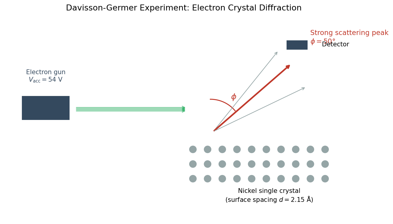
Fig. 2.4: Schematic diagram of the Davisson-Germer experiment. An electron beam accelerated through 54 V strikes a nickel single crystal (surface atomic spacing \(d = 2.15\) Å), and a strong scattering peak is observed at scattering angle \(\phi = 50°\). The wavelength can be determined from the surface atomic spacing \(d\) and scattering angle \(\phi\) using the diffraction condition.
Follow along with Fig. 2.4 "Schematic diagram of the Davisson-Germer experiment". Consider two atoms A and B separated by spacing \(d\) on the surface. Since the incident beam is perpendicular to the surface, the wavefront arrives at A and B simultaneously (zero path difference on the incident side). Next, consider the waves going out in the direction of scattering angle \(\phi\). This is exactly the same situation as a diffraction grating in high school physics—we just need to find the path difference for waves going in the same direction from adjacent scattering sources (here, atoms).
🔵 Kai: Oh, it's just the diffraction grating slits replaced by atoms?
🟡 Lina: Exactly. A and B are separated by distance \(d\) along the surface, and the scattering direction is tilted by angle \(\phi\) from the normal. Recall the diffraction grating from high school physics—when light is incident perpendicularly on slits with spacing \(d\), the path difference in the direction of angle \(\phi\) is \(d\sin\phi\). The essence is the same here. Specifically, draw lines parallel to the scattering direction from both A and B (in Fig. 2.4 "Schematic diagram of the Davisson-Germer experiment", check the triangle showing the path difference between scattered waves from the two atoms). The "offset" between these two parallel lines is the path difference. Drop a perpendicular from B to the line through A in the scattering direction, forming a right triangle. The hypotenuse of this triangle is the distance \(d\) between A and B (the spacing along the surface). Now let's check the angle relationships. The surface is at \(90°\) to the normal, so the direction of AB along the surface is perpendicular to the normal. The scattering direction is tilted by angle \(\phi\) from the normal, so the angle between the AB direction (along the surface) and the scattering direction is \(90° - \phi\). In the right triangle with hypotenuse \(d\) and one side making angle \((90° - \phi)\), the path difference (the side opposite to that angle) is \(d\sin\phi\) (using \(\sin\phi = \cos(90° - \phi)\)). Since the incident wave comes in vertically, the incident-side path difference is zero, and only the scattering-direction path difference matters. The high school diffraction grating is "transmission type" where light passes through slits, but here it's "reflection type" where surface atoms are the scattering sources—but the path difference geometry is exactly the same. Constructive interference occurs when this path difference equals an integer multiple of the wavelength:
This has the same form as the diffraction grating formula from high school physics. But be careful—in the high school diffraction grating, the angle is often measured from the normal to the grating surface, but here \(\phi\) is measured as the angle between the incident direction and the scattered direction. Since the incidence is along the normal direction, the angle from the normal and the angle from the incident direction coincide. The Bragg condition (2.15) that comes up later deals with reflection from crystal "layers" and uses a different angle convention, so don't confuse them.
⚪ Mei: Even with the same \(d\sin\phi = n\lambda\), the angle definitions differ between experiments, so we need to be careful.
🟡 Lina: Substituting \(n = 1\), \(\phi = 50°\):
⚪ Mei: Substituting \(V_{\mathrm{acc}} = 54\) V into equation (2.12) gives \(\lambda \approx 1.226/\sqrt{54} \approx 1.67\) Å. That nearly matches the experimental value of \(1.65\) Å!
🔵 Kai: Wow, that's almost exactly right...!
🟡 Lina: Yes. The wavelength predicted by de Broglie's formula (2.11) and the wavelength measured from diffraction agree beautifully. This was the first experimental confirmation of the de Broglie hypothesis.
What This Experiment Demonstrates
🟡 Lina: Let me summarize the significance of the Davisson-Germer experiment.
- Electrons definitely behave as waves and diffract from crystal lattices
- The wavelength obtained from diffraction matches de Broglie's prediction \(\lambda = h/p\)
- The hypothesis that "matter particles possess wave nature" has been experimentally confirmed
🔵 Kai: It's symmetric with how light's particle nature was confirmed by Compton scattering. Now, conversely, particles' wave nature has been confirmed.
🟡 Lina: Nice organization. Let's display the symmetry in a table.
Table 2.2: Symmetry of major experiments demonstrating wave and particle nature
| Experiment | What it demonstrated |
|---|---|
| Photoelectric effect (1905) | Light has particle nature (\(E = h\nu\)) |
| Compton scattering (1923) | Photons have momentum (\(p = h/\lambda\)) |
| Davisson-Germer (1927) | Electrons have wave nature (\(\lambda = h/p\)) |
✅ Comprehension Check: In the Davisson-Germer experiment, if the accelerating voltage is increased from 54 V to 100 V, what happens to the diffraction peak angle? (Does it increase? Decrease?)
Answer
Increasing the accelerating voltage increases the momentum \(p\), making the de Broglie wavelength \(\lambda = h/p\) shorter. In equation (2.13), when \(\lambda\) decreases, \(\sin\phi\) also decreases, so the diffraction peak angle \(\phi\) decreases.
📝 Exercises:
- Reproducing the Davisson-Germer experiment calculations → Problem M-2. Reproduction Calculation of the Davisson-Germer Experiment
2.5 Electron Diffraction — G. P. Thomson's Experiment and the Bragg Condition
🟡 Lina: Almost simultaneously with the Davisson-Germer experiment (in 1928), G. P. Thomson in England confirmed electron wave behavior using a different method.
🔵 Kai: Thomson—is he related to J. J. Thomson who discovered the electron?
🟡 Lina: Good question. G. P. Thomson was J. J. Thomson's son. The father discovered the electron as a "particle," and the son demonstrated the electron's "wave nature." A beautiful episode in the history of physics.
Experimental Method
🟡 Lina: G. P. Thomson's experiment took a different approach from Davisson-Germer.
- A high-speed electron beam (accelerated through tens of thousands of volts) is passed through a thin metal foil (gold or aluminum)
- Electrons transmitted through the metal foil are detected on a photographic plate
- Concentric ring patterns (diffraction rings) appear on the photographic plate
🔵 Kai: Why do rings form?
🟡 Lina: The metal foil is polycrystalline—meaning tiny crystal grains are gathered together in random orientations. Only those crystal grains satisfying the diffraction condition (which I'll explain shortly as the "Bragg condition") contribute to diffraction, but since the grain orientations are random, the diffracted light spreads out in a cone around the incident direction. Cutting this with a plane gives circles (rings). In other words, whether the sample is single crystal or polycrystalline changes the shape of the diffraction pattern.
⚪ Mei: I see—in Davisson-Germer it was a single crystal so peaks appear at specific angles, and here with polycrystal you get rings.
🟡 Lina: Right. The crystal structure determines the pattern shape. A schematic is shown in Fig. 2.5 "Schematic of G". In fact, the ring patterns from electron diffraction look very similar to X-ray diffraction patterns. If the wavelength is the same, both X-rays and electrons produce the same diffraction pattern—clear evidence that electrons behave as waves.
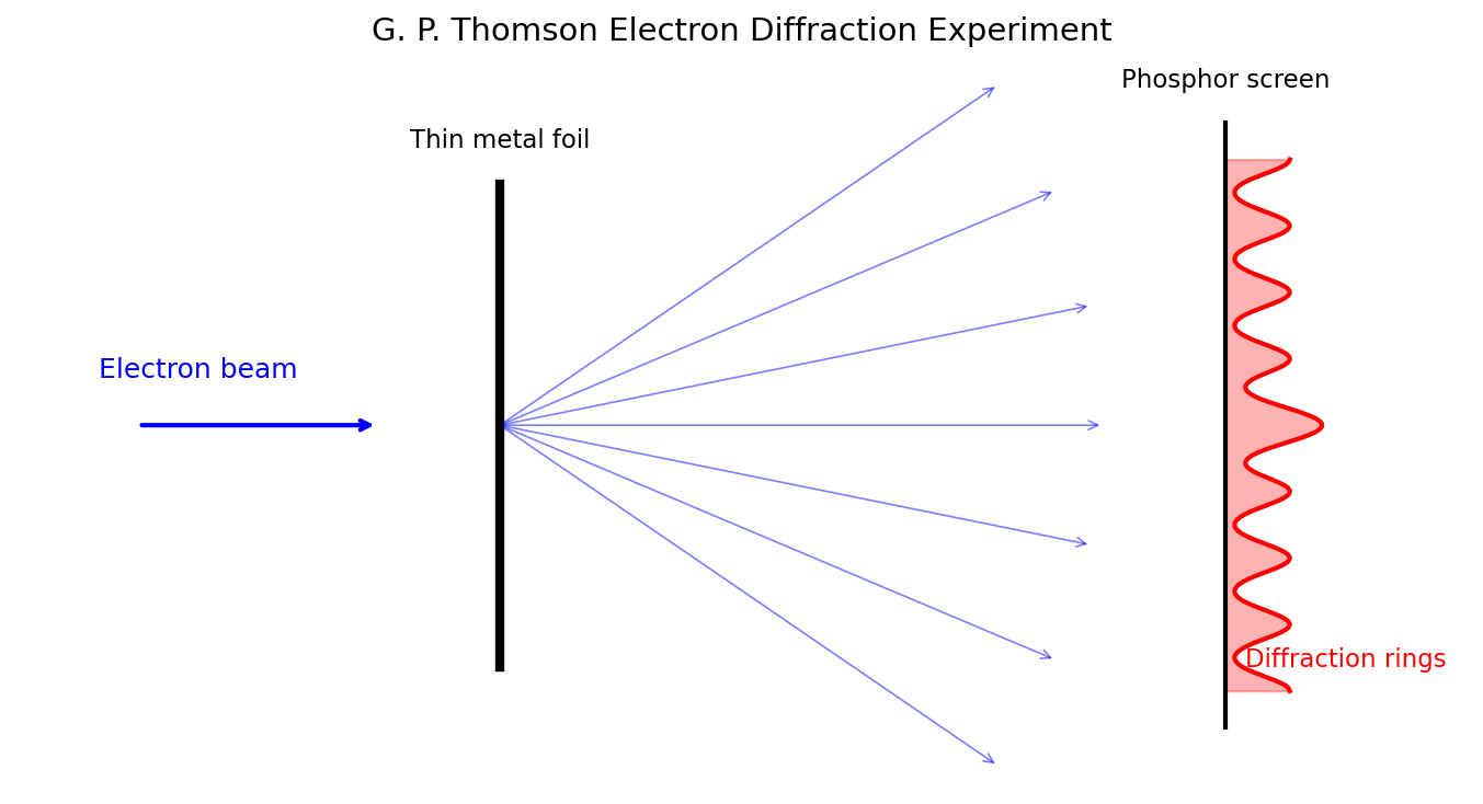
Fig. 2.5: Schematic of G. P. Thomson's electron diffraction experiment. A high-energy electron beam passes through a polycrystalline metal foil and forms concentric diffraction rings on a photographic plate. Crystal grains at random orientations in the polycrystal satisfy the Bragg condition, causing diffracted beams to spread conically and form ring patterns.
Review of the Bragg Condition
🟡 Lina: Let's review the basic condition for diffraction by crystals. A crystal is a structure with atoms arranged regularly, with layers of atoms stacked at uniform spacing \(d\). When a wave is reflected by each layer, the condition for constructive interference of reflected waves from adjacent layers is:
Here: - \(d\): spacing between crystal planes - \(\theta\): angle between the crystal plane and the incident direction (called the glancing angle. When the wave comes in nearly parallel to the surface ("grazing"), \(\theta\) is small; as it approaches perpendicular to the surface, \(\theta\) increases. In high school physics, the "angle of incidence" is measured from the normal, but Bragg's \(\theta\) is measured from the plane—so if the high school angle of incidence is \(\alpha\), then \(\theta = 90° - \alpha\). Also, the \(\phi\) in the Davisson-Germer experiment was "the angle between the incident and scattered directions," so the angle definitions differ.) - \(n\): a positive integer (the order of diffraction) - \(\lambda\): wavelength
This is called the Bragg condition.
🔵 Kai: Why is it \(2d\sin\theta\)?
🟡 Lina: Let me explain with a diagram. Look at Fig. 2.6 "Geometric explanation of the Bragg condition". Consider two adjacent crystal planes. Comparing the path of a wave reflected from the upper plane with one that goes down to the lower plane and reflects, the wave taking the lower path travels an extra distance of \(2d\sin\theta\). When this extra path difference is an integer multiple of the wavelength, the two reflected waves are in phase and constructively interfere.
⚪ Mei: Path difference = integer multiple of wavelength → crests align → constructive interference. This is the same reasoning as the interference condition in high school physics.
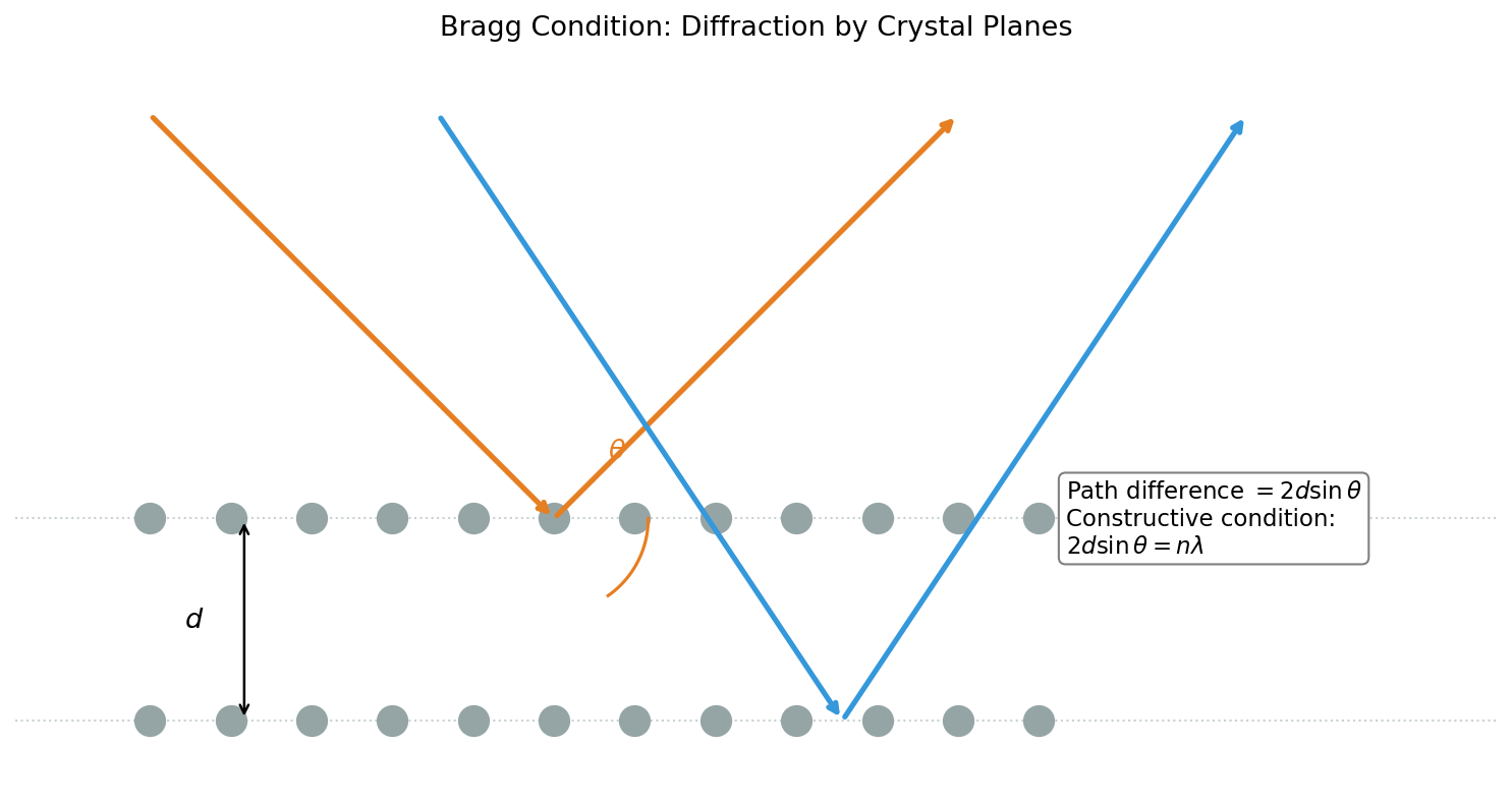
Fig. 2.6: Geometric explanation of the Bragg condition. The path difference for waves reflected from two layers with crystal plane spacing \(d\) is \(2d\sin\theta\). When this path difference equals an integer multiple of the wavelength \(n\lambda\), the reflected waves constructively interfere and a diffraction peak appears.
🟡 Lina: Right. The Bragg condition holds for any wave—X-rays, electrons, or neutrons. So the fact that electrons diffract according to the Bragg condition is direct evidence that electrons behave as waves. Let me compare the Davisson-Germer experiment and G. P. Thomson's experiment here.
Table 2.3: Comparison of the Davisson-Germer and G. P. Thomson experiments
| Item | Davisson-Germer (1927) | G. P. Thomson (1928) |
|---|---|---|
| Electron energy | Low energy (~54 V) | High energy (tens of thousands of V) |
| Sample | Nickel single crystal (surface reflection) | Thin metal film (transmission) |
| Diffraction condition | Surface grating formula \(d\sin\phi = n\lambda\) | Bragg condition \(2d\sin\theta = n\lambda\) |
| Pattern | Peaks at specific angles | Concentric rings |
| Sample crystallinity | Single crystal | Polycrystalline |
✅ Comprehension Check: Why does the diffraction pattern in G. P. Thomson's electron diffraction experiment form concentric rings?
Answer
The metal foil is polycrystalline, with tiny crystal grains oriented in random directions. Since crystal grains satisfying the Bragg condition exist at various orientations, the diffracted beams spread conically around the incident direction. When this cone is cut by a plane (the photographic plate), it is observed as concentric ring patterns.
Neutron Diffraction — Further Confirmation
🟡 Lina: It's not just electrons—the same phenomenon has been confirmed with neutrons. From 1936 onward, it was demonstrated that when neutrons from a nuclear reactor are directed at crystals, diffraction patterns following the Bragg condition are indeed obtained.
🔵 Kai: Neutrons have no electric charge, right? Do they still have wave properties?
🟡 Lina: They do. De Broglie's relation \(\lambda = h/p\) holds regardless of whether the particle is charged or not. As long as there's mass and velocity, the wavelength is determined. In fact, neutron diffraction is widely used in crystal structure research. Being uncharged is actually an advantage—they can penetrate deep into matter.
⚪ Mei: So matter waves are not limited to electrons but universally apply to all matter particles.
🟡 Lina: Exactly. Diffraction has been confirmed for protons, atoms, and even molecules. In 1999, a diffraction experiment with fullerene (\(\mathrm{C}_{60}\), a molecule consisting of 60 carbon atoms) succeeded. De Broglie's hypothesis has been verified over a very wide range.
✅ Comprehension Check: What property of de Broglie's relation \(\lambda = h/p\) is demonstrated by the fact that it also holds for uncharged neutrons?
Answer
De Broglie's relation holds regardless of whether a particle is charged or not—as long as there is mass and velocity (momentum), the wavelength is determined. This shows that matter waves are not an electromagnetic property but a universal property possessed by all matter particles.
✅ Comprehension Check: In the Bragg condition \(2d\sin\theta = n\lambda\), what is the wavelength of the diffracted wave when \(d = 2.0\) Å, \(\theta = 30°\), and \(n = 1\)?
Answer
\(\lambda = 2d\sin\theta / n = 2 \times 2.0 \times \sin 30° / 1 = 2 \times 2.0 \times 0.5 = 2.0\) Å.
📝 Exercises:
- Electron diffraction calculations using the Bragg condition → Problem M-4. Analysis of Electron Diffraction Using the Bragg Condition
2.6 The Essence of Wave-Particle Duality — Matter Is Neither Wave Nor Particle
🟡 Lina: Let me summarize what we've covered so far.
Table 2.4: Evidence for wave-particle duality of light and matter
| Subject | Evidence of wave nature | Evidence of particle nature |
|---|---|---|
| Light | Interference and diffraction (Young's experiment, etc.) | Photoelectric effect, Compton scattering |
| Electrons | Davisson-Germer, G. P. Thomson | Detected as particles (tracks, etc.) |
🔵 Kai: So both light and electrons are "waves and also particles." But... what does that actually mean? Waves and particles are completely different things, aren't they?
🟡 Lina: A very good question. This is actually the most important point. Here's the answer:
Electrons and photons are neither "waves" nor "particles." They are "something" that follows certain mathematical rules, and depending on how you experiment, wave-like properties or particle-like properties manifest.
⚪ Mei: So the question "wave or particle?" itself is inappropriate?
🟡 Lina: Yes. "Wave" and "particle" are concepts borrowed from classical physics that cannot fully describe entities in the microscopic world. An electron is not a "tiny billiard ball," nor is it a "wave on a water surface." A new mathematical framework is needed.
🔵 Kai: What are these "mathematical rules"?
🟡 Lina: That's precisely what we'll construct step by step in the coming chapters. First, in the next chapter, we'll analyze the double-slit experiment in detail and formally introduce the concept of "probability amplitude." From there, through the rules of probability amplitudes (Ch. 4), two-state systems (Chapters 5–6), we'll ultimately arrive at the wave function and the Schrödinger equation (Ch. 7).
What Is "Behaving as a Wave"?
🟡 Lina: Let me clear up a common misconception here. When you hear "the electron spreads out like a wave," you might imagine "the electron is like a thin cloud spread across space." But that's not it.
🔵 Kai: It's not?
🟡 Lina: When you detect an electron with a detector, it's always detected at a single point, as one whole electron. It never happens that "half the electron is here and the other half is there."
🔵 Kai: Then what is behaving as a wave?
🟡 Lina: "The amplitude of the probability of finding the electron there" is what behaves as a wave. This is called the probability amplitude. The probability amplitude can interfere, diffract, and superpose—it has wave properties. But when actually detected, the particle appears at a single point with a probability proportional to the square of the magnitude of the probability amplitude (precisely, "the absolute value squared"—we'll define this in detail from the next chapter onward).
🔵 Kai: "A wave of probability"... Probabilities interfering means that probabilities can cancel each other out instead of just adding up?
🟡 Lina: Exactly. Because "probability amplitudes" are added rather than probabilities themselves, cancellation (destructive interference) can occur. But we'll see the details concretely in the next chapter through the double-slit experiment. For now, just remember the following:
- Matter particles possess wave nature (experimental fact)
- Wave nature is described as a wave of "probability amplitude"
- Detection always occurs "as a particle at a single point"
- A new framework that unifies these is needed
✅ Comprehension Check: In the wave nature of electrons, what is "behaving as a wave"? Is the electron itself spread out across space?
Answer
What behaves as a wave is "the amplitude of the probability of finding the electron there" (probability amplitude), not the electron itself being spread thinly across space. When an electron is detected, it is always found as one whole particle at a single point. The probability amplitude has wave properties such as interference and diffraction, and its absolute value squared gives the detection probability.
✅ Comprehension Check: Explain why the expression "the electron is a wave" is inaccurate.
Answer
When an electron is detected, it is always found as one whole particle at a single point. What "behaves as a wave" is not the electron itself but the amplitude of the probability of finding the electron (probability amplitude). The electron is neither a "wave" nor a "particle" but a new kind of entity that follows the rules of probability amplitudes.
2.7 Preview of the Uncertainty Principle — What the de Broglie Wavelength Implies
🟡 Lina: De Broglie's relation \(\lambda = h/p\) has one more deep implication. Let's take a brief peek at it to close out.
🔵 Kai: There's more?
🟡 Lina: Waves have a fundamental property: the more well-defined the wavelength, the more the wave is spread out in space. Conversely, the more localized a wave is in a narrow region, the more uncertain its wavelength becomes.
🔵 Kai: Huh, why? ...Oh, but actually, a perfect sine wave repeats the same shape forever—like \(\sin(kx)\), oscillating at the same amplitude no matter how far \(x\) goes. In that case, you can't tell "where the wave is"... But conversely, when you want to confine a wave to a narrow region, why do you need "various wavelengths"?
🟡 Lina: Good question. Let's think about it with a familiar example. You learned about "beats" in high school physics, right? When you simultaneously sound two tuning forks with slightly different frequencies, the sound gets louder and softer. That's because two waves overlap, constructively interfering at some times and destructively interfering at others.
🔵 Kai: Ah, the same thing happens in space too?
🟡 Lina: Exactly. Beats are a phenomenon where amplitude varies in the "time direction," but exactly the same mathematics applies in the "spatial direction." Imagine this concretely. If you overlap two waves with slightly different wavelengths in space—say a wave with wavelength 10 cm and one with wavelength 11 cm—at some locations the crests align and the amplitude is large, while at other locations crests and troughs cancel and the amplitude is small. Just as beats make sound louder and softer, the same thing happens along position in space.
🔵 Kai: Oh, spatial beats! Just mixing two wavelengths creates a situation where "amplitude is large here and small there." But beats repeat periodically, right? Can you really concentrate things in one spot with just that?
🟡 Lina: Good observation. Actually, with just two wavelengths, like beats, the strong and weak pattern repeats periodically—you can't concentrate it in "just one spot." But as you add more varieties—3, 4, and more wavelengths—you can arrange it so that at one particular spot all the waves align their crests and constructively interfere, while everywhere else the phases are scattered and cancel out.
⚪ Mei: The more wavelength varieties there are, the more efficient the "cancellation" becomes, and the sharper the localization.
🟡 Lina: Right. The reason is that waves with slightly different wavelengths have different phase shifts at each position, so at locations other than "where everyone aligns," some waves are cresting while others are troughing, and they cancel each other out. The more wavelength varieties you include, the more efficient the "cancellation" becomes, and the region where amplitude concentrates gets narrower and narrower. In other words, to create a wave confined to a narrow region, you need to superpose waves of many wavelengths—the wavelength becomes indeterminate. This is a mathematical property of waves that holds independently of quantum mechanics. A localized wave cannot be represented by a single wavelength, so the wavelength becomes uncertain. Moreover, the narrower the confinement, the more wavelength components are needed.
🔵 Kai: So "localization ↔ wavelength uncertainty" is determined just by the properties of waves. This is a pre-quantum mechanics fact...
🟡 Lina: Right. And now recall de Broglie's relation \(p = h/\lambda = \hbar k\). The uncertainty in wavelength directly translates to uncertainty in momentum. That is:
- Position well-defined in a narrow range → wave is localized → wavelength (= momentum) is uncertain
- Momentum well-defined → wavelength is fixed → wave is spread out → position is uncertain
Let's confirm this visually. Look at Fig. 2.7 "Relationship between wave packet localization and wavelength (momentum)". On the left is a "narrow wave packet"—many wavelengths superposed to concentrate in one place—where position is well-defined but many wavelength components are mixed in (= momentum is uncertain). On the right is a "broad wave packet"—nearly a single-wavelength sine wave—where momentum is well-defined but you can't tell where the wave is (= position is uncertain). Compare left and right.
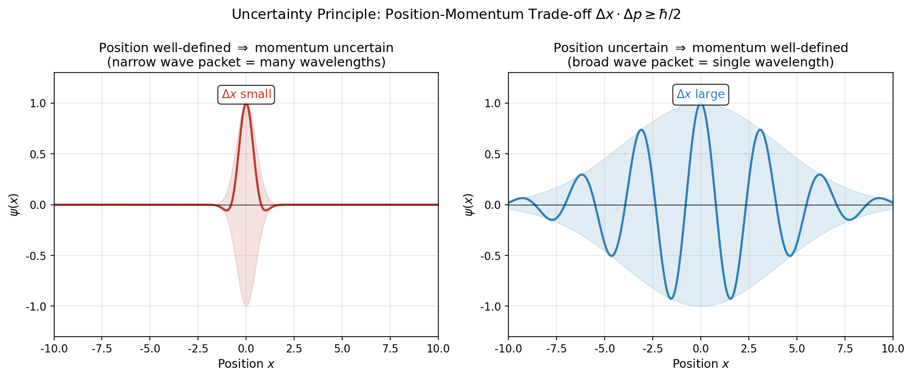
Fig. 2.7: Relationship between wave packet localization and wavelength (momentum). Left: A narrow wave packet requires many wavelength components to construct, so momentum is uncertain. Right: A broad wave packet is close to a single wavelength, so momentum is well-defined but position is uncertain. This is the intuitive meaning of Heisenberg's uncertainty relation \(\Delta x\cdot\Delta p\geq\hbar/2\).
🔵 Kai: Position and momentum can't both be determined precisely at the same time...! But isn't that just because the measuring instruments aren't precise enough? Couldn't you measure both accurately with better equipment?
🟡 Lina: That question is natural, but the answer is "no." This isn't a limitation of measurement technology but a fundamental property of nature. As long as de Broglie's relation \(p = \hbar k\) is correct, simultaneous determination of position and momentum is impossible in principle due to the mathematical properties of waves. Quantitatively, this is expressed as Heisenberg's uncertainty principle:
The rigorous derivation of this inequality will be given in Ch. 8.
⚪ Mei: So the de Broglie wavelength formula contains the seed of the uncertainty principle.
Relation to Atomic Stability
🟡 Lina: In Ch. 1, we raised the question "why doesn't the electron fall into the nucleus?" Using the uncertainty principle, we can give an intuitive answer.
If an electron is confined near the nucleus (within a region of radius \(a\)), the position uncertainty is \(\Delta x \sim a\). From the uncertainty principle \(\Delta x \cdot \Delta p \geq \hbar/2\), the momentum uncertainty is at least:
(Since we're doing an order-of-magnitude estimate here, we won't worry about numerical factors like \(1/2\) and proceed with \(\Delta p \sim \hbar/a\). The symbol "\(\sim\)" means "of the same order of magnitude," ignoring factors of 2 or \(1/2\). What matters is whether the final atomic size comes out at the right order.)
🔵 Kai: I understand there's momentum uncertainty, but why does that lead to kinetic energy? Being uncertain doesn't mean it actually has energy, does it?
🟡 Lina: Good question. There's an important point here. If an electron is confined within a region of radius \(a\), the average value of momentum is zero (no preferred direction)—imagine a ball bouncing around inside a box. It goes right and left, so the average velocity is zero, but the speed (magnitude of velocity) isn't zero, right?
🔵 Kai: Oh, I see. Even if the average is zero, it's actually moving so there is kinetic energy!
🟡 Lina: Right. Since kinetic energy is \(p^2/(2m_e)\), if the "magnitude" of momentum isn't zero, the energy remains. As an analogy with test scores: consider a class with one person scoring +50 and another scoring −50. The average is \((50 + (-50))/2 = 0\), but the average of the squared scores is \((50^2 + (-50)^2)/2 = 2500\), which isn't zero, right?
🔵 Kai: Oh, that's true. Even when the average is zero, the average of the squares isn't zero!
🟡 Lina: Similarly, even if the average momentum is zero, if there's spread \(\Delta p\), then "the average of \(p^2\)" is on the order of \((\Delta p)^2\). In physics, we denote averages with angle brackets \(\langle \cdot \rangle\)—for example, \(\langle p \rangle\) means "the average value of \(p\)" and \(\langle p^2 \rangle\) means "the average value of \(p^2\)." \(\Delta p\) is the width of the spread (the standard deviation in statistics). In general, "average of the square = square of the average + square of the spread" holds: \(\langle p^2 \rangle = \langle p \rangle^2 + (\Delta p)^2\).
🔵 Kai: Where does that formula come from?
🟡 Lina: In high school statistics you learned "variance = average of (each datum − mean)\(^2\)," right? Writing that as a formula: \(V = \langle (X - \mu)^2 \rangle\). Expanding the bracket: \(\langle X^2 - 2\mu X + \mu^2 \rangle = \langle X^2 \rangle - 2\mu\langle X \rangle + \mu^2\), and since \(\langle X \rangle = \mu\), we get \(V = \langle X^2 \rangle - \mu^2\). Rearranging: \(\langle X^2 \rangle = \mu^2 + V\)—that is, "average of the square = square of the average + square of the spread."
🔵 Kai: Oh, checking with the earlier test score example... average \(\mu = 0\), spread \(\Delta X = 50\), so \(\langle X^2 \rangle = 0 + 50^2 = 2500\). Direct calculation also gives \((50^2 + 50^2)/2 = 2500\)—they match!
🟡 Lina: So if \(\langle p \rangle = 0\), then \(\langle p^2 \rangle = (\Delta p)^2\). Since kinetic energy is \(T = p^2/(2m_e)\), its average is \(\langle T \rangle = \langle p^2 \rangle/(2m_e) = (\Delta p)^2/(2m_e)\).
⚪ Mei: The spread directly becomes the source of kinetic energy.
🟡 Lina: Perfect summary. Substituting \(\Delta p \sim \hbar/a\):
Meanwhile, the potential energy from Coulomb attraction is (using the high school formula \(V = kq_1 q_2/r\) with \(k = 1/(4\pi\varepsilon_0)\), nuclear charge \(q_1 = +e\), electron charge \(q_2 = -e\)):
Looking at the total energy \(E = T + V\) as a function of \(a\):
🔵 Kai: If you make \(a\) smaller, the potential energy decreases, but the kinetic energy rises as \(1/a^2\), so... if you make it too small, the energy actually increases! That means it "can't fall in"?
🟡 Lina: Exactly. Look at the graph in Fig. 2.8 "Atomic stability from the uncertainty principle". In the small-\(a\) region, kinetic energy diverges as \(1/a^2\), and in the large-\(a\) region, the gain from potential energy diminishes. The competition between these two means the total energy has a minimum.
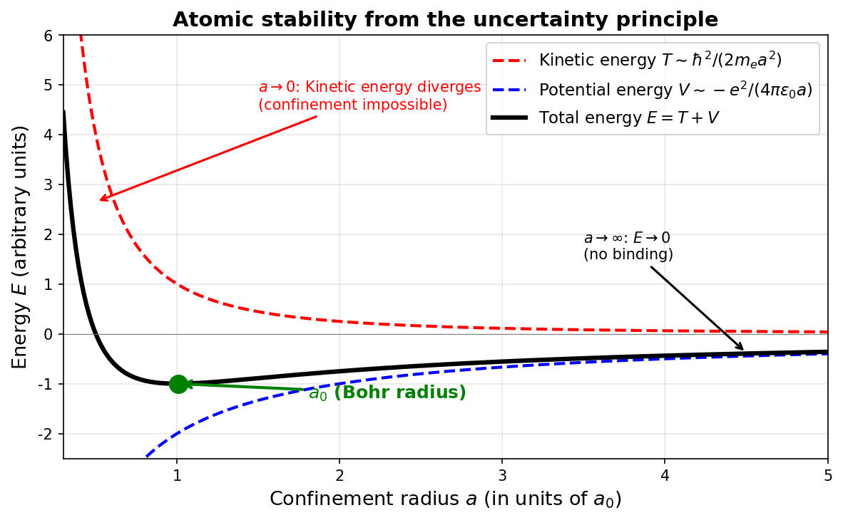
Fig. 2.8: Atomic stability from the uncertainty principle. As the confinement radius \(a\) decreases, kinetic energy \(T \sim \hbar^2/(2m_e a^2)\) rises steeply; as \(a\) increases, the potential energy gain diminishes. The minimum of total energy \(E = T + V\) gives the Bohr radius \(a_0\).
🟡 Lina: Let's minimize \(E(a)\). The derivative of \(a^{-2}\) with respect to \(a\) is \(-2a^{-3}\), and the derivative of \(a^{-1}\) is \(-a^{-2}\) (just using the power rule \((a^n)' = na^{n-1}\)). Setting \(dE/da = 0\): the derivative of the first term is \(\frac{\hbar^2}{2m_e} \times (-2a^{-3}) = -\frac{\hbar^2}{m_e a^3}\); differentiating the second term \(-\frac{e^2}{4\pi\varepsilon_0}\cdot a^{-1}\) gives \(-\frac{e^2}{4\pi\varepsilon_0} \times (-1)\cdot a^{-2} = +\frac{e^2}{4\pi\varepsilon_0 a^2}\) (minus times minus equals plus):
🔵 Kai: So we set this equal to zero and solve for \(a\).
🟡 Lina: Right. Rearranging:
Multiplying both sides by \(a^3\):
Therefore:
⚪ Mei: It's remarkable that just an order-of-magnitude estimate gives the size of a hydrogen atom.
🟡 Lina: This is the value called the Bohr radius, a measure of the size of a hydrogen atom. Thanks to the uncertainty principle, the electron cannot fall into the nucleus—if it tried, the kinetic energy would diverge. This isn't a rigorous derivation but just an "estimate," yet it gives the correct order of magnitude. The rigorous calculation will be done in Ch. 16 (the hydrogen atom).
✅ Comprehension Check: According to the uncertainty principle, how does kinetic energy behave when an electron is confined to a region of radius \(a\)?
Answer
Kinetic energy increases as \(T \sim \hbar^2/(2m_e a^2)\), inversely proportional to \(a^2\). The smaller \(a\) becomes, the more rapidly kinetic energy grows, making it impossible to confine the electron to an infinitely small region.
2.8 Summary of This Chapter
🟡 Lina: Let's summarize today's content.
The Einstein-de Broglie Relations
For all matter particles, the following relations hold:
Experimental Confirmation
Table 2.5: Experimental confirmation of the Einstein–de Broglie relations
| Experiment | Year | What was confirmed |
|---|---|---|
| Compton scattering | 1923 | Photon momentum \(p = h/\lambda\) |
| Davisson-Germer | 1927 | Electron de Broglie wavelength \(\lambda = h/p\) |
| G. P. Thomson | 1928 | Electron diffraction rings |
| Neutron diffraction | 1936– | Wave nature of neutrons |
| \(\mathrm{C}_{60}\) diffraction | 1999 | Wave nature of large molecules |
Core Messages
- Matter particles possess wave nature — this is experimental fact
- Wave nature is described as a wave of probability amplitude — the particle itself does not "spread out"
- Detection always occurs as a particle at a single point — the absolute value squared of the probability amplitude gives the detection probability
- De Broglie's relation is the root of the uncertainty principle — through \(p = \hbar k\), wave localization and momentum definiteness become a trade-off
- A new mathematical framework is needed — a description that transcends the "wave or particle" dichotomy
Preview of the Next Chapter
🟡 Lina: In the next chapter, we'll analyze in detail the most dramatic stage for wave-particle duality—the double-slit experiment. What happens when electrons are sent through slits one at a time? How do "probability amplitudes" interfere? And how does observation change the outcome?
🔵 Kai: That's the "collapse of determinism and realism" that was previewed at the end of Ch. 1.
🟡 Lina: Yes. The double-slit experiment is the one Feynman called "the experiment that contains all the mysteries of quantum mechanics." Now that we have the concept of de Broglie wavelength, we can finally delve into its heart.
⚪ Mei: What it means for probability amplitudes to interfere—that's the theme of the next chapter.
Practice Problems
📝 Exercises:
- Calculation of Compton scattering wavelength shift → Problem B-2. In the Compton scattering formula (2.1), find the wavelength shift for scattering angle
- Calculating de Broglie wavelengths for various particles → Problem B-3. Find the de Broglie wavelength of a proton with mass kg moving at velocity m/s
- Reproducing the Davisson-Germer experiment calculations → Problem M-2. Reproduction Calculation of the Davisson-Germer Experiment
- Electron diffraction calculations using the Bragg condition → Problem M-4. Analysis of Electron Diffraction Using the Bragg Condition
References
- R. P. Feynman, R. B. Leighton, M. Sands, The Feynman Lectures on Physics, Vol. III, Ch. 1–2(Intuitive discussion of wave-particle duality and the uncertainty principle)
- 広江克彦『趣味で量子力学』Ch. 2–3(Careful exposition of de Broglie waves and wave-particle duality)
- D. J. Griffiths, Introduction to Quantum Mechanics, 3rd ed., Ch. 1(Introduction to de Broglie relations and the statistical interpretation)
- C. Rovelli, Reality Is Not What It Seems, Ch. 6(Historical context of the light quantum hypothesis and matter waves)
Feedback on this page
Let us know if something was unclear, incorrect, or could be improved.