Chapter 5: Quantization of the Dirac Field — Anticommutation Relations for Fermions
Story so far:
In Ch. 4, we carried out the canonical quantization of the real scalar field. By promoting fields to operators and imposing the equal-time commutation relation \([\hat{\phi}(\boldsymbol{x}), \hat{\pi}(\boldsymbol{y})] = i\delta^{(3)}(\boldsymbol{x} - \boldsymbol{y})\), creation and annihilation operators \(\hat{a}^\dagger_{\boldsymbol{p}}, \hat{a}_{\boldsymbol{p}}\) emerged, and we saw that field excitations can be interpreted as "particles." We confirmed the structure of Fock space and that Bose-Einstein statistics naturally follow from the commutation relations.
Goals of this chapter
- Quantize the Dirac field (a spin-\(1/2\) field)
- Experience the fatal breakdown that occurs when commutation relations are imposed following the same procedure as for the scalar field—energy becomes unbounded below—and understand that anticommutation relations are unavoidable as the remedy
- Confirm that the Pauli exclusion principle and Fermi-Dirac statistics naturally follow from anticommutation relations, and learn about the fermionic Fock space, antiparticles, and \(C, P, T\) transformations
5.1 Review of the Dirac Equation — The Necessity of 4-Component Spinors
🟡 Lina: In Ch. 4, we quantized the scalar field—a spin-0 field. But the particles that make up matter in nature—electrons, quarks, neutrinos—are all spin-\(1/2\) particles. Today, we'll finally quantize the Dirac field, which describes these particles.
🔵 Kai: The Dirac equation was previewed in Quantum Mechanics Ch. 27, right? The idea was to "factorize" the Klein-Gordon equation to create an equation that's first-order in time derivatives.
🟡 Lina: Good memory. Let's review. The starting point is the relativistic energy-momentum relation
which, when operators are substituted, gives the Klein-Gordon equation
In natural units \(\hbar = c = 1\), this becomes
This is a second-order equation in time, and it had the problem that the probability density could become negative.
🔵 Kai: So Dirac wanted to make the time derivative first-order.
⚪ Mei: The "second-order derivative" was the problem, so he wanted to make it first-order.
🟡 Lina: Right. Dirac's idea was this: if we want first-order time derivatives, we'd like to write the "square root" of \(E^2 = |\boldsymbol{p}|^2 + m^2\) as \(E = \sqrt{|\boldsymbol{p}|^2 + m^2}\) and substitute operators to get the equation \(i\partial_t \psi = \sqrt{-\nabla^2 + m^2}\,\psi\). But with a differential operator inside the square root, a Taylor expansion would produce derivatives of infinite order, making it a non-local equation. So Dirac's brilliant idea was to realize the "square root" of \(\Box \equiv \partial_\mu \partial^\mu\) (the d'Alembertian) using matrices. Specifically, he introduced 4 matrices \(\gamma^\mu\) such that
holds. This way, \(\gamma^\mu \partial_\mu\) is a first-order differential operator, so we can write a first-order equation \((\gamma^\mu \partial_\mu + \text{constant})\psi = 0\).
🔵 Kai: Expanding \((\gamma^\mu \partial_\mu)^2\) gives \(\gamma^\mu \gamma^\nu \partial_\mu \partial_\nu\), right? Since partial derivatives commute, \(\partial_\mu \partial_\nu\) is symmetric in \(\mu, \nu\)... so does that impose some condition on \(\gamma^\mu \gamma^\nu\)?
🟡 Lina: Exactly. Since \(\partial_\mu \partial_\nu\) is symmetric, the antisymmetric part of \(\gamma^\mu \gamma^\nu\) vanishes and only the symmetric part survives. So the required condition is
That is, the anticommutation relation
Here \(\eta^{\mu\nu} = \mathrm{diag}(+1, -1, -1, -1)\) is the Minkowski metric and \(\mathbf{1}\) is the identity matrix. This relation is called the Clifford algebra.
🔵 Kai: An anticommutation relation appeared! But this is an anticommutation relation between \(\gamma\) matrices, not about field operators, right?
🟡 Lina: That's right. The anticommutation relation here is a purely algebraic property of matrices. It's distinct from the anticommutation relations that appear in field quantization. But interestingly, the structure of "anticommutation" is already lurking at the very starting point of the Dirac equation.
🟡 Lina: Let's see what we can read off concretely from equation (5.1) by plugging in values of \(\mu, \nu\).
⚪ Mei: Let me try.
- \(\mu = \nu = 0\): Since \(\eta^{00} = +1\), we get \((\gamma^0)^2 = +\mathbf{1}\)
- \(\mu = \nu = i\) (spatial components): Since \(\eta^{ii} = -1\), we get \((\gamma^i)^2 = -\mathbf{1}\)
- \(\mu \neq \nu\): Since \(\eta^{\mu\nu} = 0\), we get \(\gamma^\mu \gamma^\nu = -\gamma^\nu \gamma^\mu\) (different \(\gamma\) matrices anticommute)
There we go.
🔵 Kai: Pauli matrices are \(2 \times 2\) and there are 3 of them, but we need 4 \(\gamma\) matrices. Can't we use \(2 \times 2\)?
🟡 Lina: Good question. The space of \(2 \times 2\) matrices is spanned by the identity \(\mathbf{1}\) and the 3 Pauli matrices \(\sigma^1, \sigma^2, \sigma^3\). To satisfy the Clifford algebra, we need 4 mutually anticommuting matrices, but in \(2 \times 2\) we can only get at most 3 (the Pauli matrices are exactly that). There's no room for a fourth. So the minimum is \(4 \times 4\) matrices, and the wave function \(\psi\) has 4 components. This is the Dirac spinor.
✅ Comprehension Check: Explain why the Dirac spinor has 4 components, from the perspective of the Clifford algebra and matrix size.
Answer
To satisfy the Clifford algebra \(\{\gamma^\mu, \gamma^\nu\} = 2\eta^{\mu\nu}\), we need 4 mutually anticommuting matrices, but in \(2 \times 2\) matrices we can only get at most 3 (the Pauli matrices). A minimum of \(4 \times 4\) matrices is required, and the wave function \(\psi\) acted upon by them becomes a 4-component Dirac spinor.
The Complete Form of the Dirac Equation
🟡 Lina: Using the \(\gamma\) matrices, we can factorize the Klein-Gordon equation. Let's verify this.
First, an important note: the \(\gamma\) matrices are constant matrices that don't depend on coordinates, so the differential operator \(\partial_\mu\) passes through \(\gamma\) and acts only on \(\psi\) behind it. Therefore the ordering of \(i\), \(\gamma\), \(\partial\) can be freely rearranged.
Let's expand this term by term. Four terms appear:
- Term 1 (derivative × derivative): \((-i\gamma^\mu\partial_\mu)(i\gamma^\nu\partial_\nu) = (-i)(i)\gamma^\mu\gamma^\nu\partial_\mu\partial_\nu = +\gamma^\mu\gamma^\nu\partial_\mu\partial_\nu\) (since \((-i)(i) = -(i^2) = -(-1) = +1\))
- Term 2 (derivative × mass): \((-i\gamma^\mu\partial_\mu)(-m) = +im\gamma^\mu\partial_\mu\)
- Term 3 (mass × derivative): \((-m)(i\gamma^\nu\partial_\nu) = -im\gamma^\nu\partial_\nu\)
- Term 4 (mass × mass): \((-m)(-m) = m^2\)
Let's look at the cross terms (Term 2 + Term 3). Both \(\mu\) and \(\nu\) are dummy indices running over \(0, 1, 2, 3\) (temporary names for "sum over everything"), so \(\gamma^\mu\partial_\mu = \gamma^0\partial_0 + \gamma^1\partial_1 + \gamma^2\partial_2 + \gamma^3\partial_3\) and \(\gamma^\nu\partial_\nu = \gamma^0\partial_0 + \gamma^1\partial_1 + \gamma^2\partial_2 + \gamma^3\partial_3\) are the same thing with relabeled indices. Therefore \(+im\gamma^\mu\partial_\mu - im\gamma^\mu\partial_\mu = 0\), and the cross terms cancel. Only Term 1 and Term 4 remain. Let's process Term 1 further. Any matrix product can be decomposed into symmetric and antisymmetric parts: \(\gamma^\mu\gamma^\nu = \frac{1}{2}\{\gamma^\mu, \gamma^\nu\} + \frac{1}{2}[\gamma^\mu, \gamma^\nu]\). Substituting the Clifford algebra \(\{\gamma^\mu, \gamma^\nu\} = 2\eta^{\mu\nu}\):
Since \(\partial_\mu\partial_\nu\) is symmetric under \(\mu \leftrightarrow \nu\), its contraction with the antisymmetric part \([\gamma^\mu, \gamma^\nu]\) is zero. Thus \(\gamma^\mu\gamma^\nu \partial_\mu \partial_\nu = \eta^{\mu\nu}\partial_\mu\partial_\nu = \partial_\mu\partial^\mu\). Therefore
The factorization is confirmed. The Klein-Gordon operator \(\partial_\mu\partial^\mu + m^2\) has been decomposed into a product of two first-order operators. To obtain the Dirac equation from here, we set the right factor to zero:
This is the Dirac equation. Let me introduce the Feynman slash notation here. For any 4-vector \(A\), we define \(\not\!A \equiv \gamma^\mu A_\mu\) (contracting the \(\gamma\) matrices with the lower-index components \(A_\mu\)). Applied to the differential operator, \(\not\!\partial \equiv \gamma^\mu \partial_\mu\), and the Dirac equation can be written compactly as \((i\not\!\partial - m)\psi = 0\). We'll also use \(\not\!p \equiv \gamma^\mu p_\mu\) later.
Let's confirm that solutions of this equation also satisfy the Klein-Gordon equation. Acting on both sides of \((i\not\!\partial - m)\psi = 0\) from the left with \((-i\not\!\partial - m)\), we can directly use our factorization result \((-i\not\!\partial - m)(i\not\!\partial - m) = \partial_\mu\partial^\mu + m^2\) to get \((\partial_\mu\partial^\mu + m^2)\psi = 0\)—the Klein-Gordon equation follows. In other words, solutions of the Dirac equation automatically satisfy the Klein-Gordon equation as well. Thus
🔵 Kai: Both the time and spatial derivatives are first order! Is Lorentz covariance also satisfied?
🟡 Lina: Good question. To verify that, we need to know how \(\psi\) transforms under Lorentz transformations. Let's look at that in the next section.
✅ Comprehension Check: From the Clifford algebra \(\{\gamma^\mu, \gamma^\nu\} = 2\eta^{\mu\nu}\), derive \(\gamma^0 \gamma^1 = -\gamma^1 \gamma^0\).
Answer
For \(\mu = 0, \nu = 1\), since \(\eta^{01} = 0\), we have \(\{\gamma^0, \gamma^1\} = \gamma^0\gamma^1 + \gamma^1\gamma^0 = 0\). Therefore \(\gamma^0\gamma^1 = -\gamma^1\gamma^0\).
📝 Exercises:
- Deriving properties of \(\gamma\) matrices from the Clifford algebra → Problem B-1. Basic Calculations with the Clifford Algebra
5.2 Spinor Representations of the Lorentz Group — Spinors Are Not Vectors
🟡 Lina: In Ch. 2, we learned how fields transform under Lorentz transformations. Recall that a scalar field transforms as \(\phi(x) \to \phi'(x) = \phi(\Lambda^{-1}x)\)—meaning "to find the field value at point \(x\) in the transformed frame, bring the value from the corresponding point \(\Lambda^{-1}x\) in the original frame" (this is the "active transformation" perspective we learned in Ch. 2—the coordinate system stays fixed while the physical system is moved). A vector field transforms as \(A^\mu(x) \to \Lambda^\mu{}_\nu A^\nu(\Lambda^{-1}x)\), with not only the coordinate argument changing but also mixing among the components. So how does the Dirac spinor \(\psi\) transform?
🔵 Kai: Since it has 4 components, does it transform like a vector with \(\Lambda^\mu{}_\nu\)... or not?
🟡 Lina: No. Spinors are fundamentally different objects from vectors. The most obvious difference is:
Rotating a vector by \(360°\) returns it to its original state. But rotating a spinor by \(360°\) reverses its sign, and only a \(720°\) rotation returns it to its original state.
🔵 Kai: Wait, a \(360°\) rotation doesn't bring it back? Is that physically possible?
🟡 Lina: It was actually confirmed in the 1975 neutron interferometry experiment by Rauch et al. A neutron beam was split in two, one half was rotated in a magnetic field, and then they were recombined. A \(360°\) rotation reversed the interference pattern, and a \(720°\) rotation restored it. Recall the properties of spin \(1/2\) from quantum mechanics. With the rotation operator \(D(\boldsymbol{\theta}) = e^{-\frac{i}{2}\boldsymbol{\sigma}\cdot\boldsymbol{\theta}}\) using Pauli matrices \(\boldsymbol{\sigma}\), substituting \(\theta = 2\pi\) (\(360°\)) rotation about the \(z\)-axis gives \(e^{-i\pi\sigma^3} = \cos\pi \cdot \mathbf{1} - i\sin\pi \cdot \sigma^3 = -\mathbf{1}\), right?
🔵 Kai: Because there's a factor of \(1/2\) in the exponent of the rotation operator, rotating by \(2\pi\) only advances the phase by \(\pi\), giving \(-\mathbf{1}\). But if only the sign flips, is it physically observable? The overall phase shouldn't be measurable...
🟡 Lina: Good observation. Indeed, the overall phase can't be measured. But in interference experiments, we measure the relative phase between two paths, so if only one path is rotated by \(360°\), the interference pattern reverses—that's exactly what Rauch's experiment observed.
⚪ Mei: So the \(e^{-i\pi\sigma^3} = -\mathbf{1}\) that Lina just showed is for \(\theta = 2\pi\), and if we plug in \(\theta = 4\pi\) into the same formula we get \(e^{-2i\pi} = +1\) and it returns to the original—so \(720°\) is needed. The factor of \(1/2\) in the exponent is the root of everything.
Decomposition of the Lorentz Algebra — Two Copies of \(\mathfrak{su}(2)\)
🟡 Lina: Let's look more deeply at the structure of the Lorentz group. As we learned in Ch. 2, there are 2 types of Lorentz transformations—spatial rotations (3 generators for 3 axes) and boosts to different inertial frames (3 generators for 3 directions). Let's write the respective generators as rotation generators \(\mathbf{J} = (J^1, J^2, J^3)\) and boost generators \(\mathbf{K} = (K^1, K^2, K^3)\). A "generator" is an operator that produces infinitesimal transformations—in the same sense that angular momentum \(\hat{L}_z\) generates infinitesimal rotations about the \(z\)-axis in quantum mechanics. \(J^i\) generates spatial rotations, and \(K^i\) generates boosts. Specifically, an infinitesimal rotation in the \(xy\)-plane is generated by \(J^3\), and an infinitesimal boost in the \(x\)-direction is generated by \(K^1\)—meaning \(J^i\) corresponds to rotation about the \(i\)-axis, and \(K^i\) corresponds to a boost in the \(i\)-direction. There are 6 in total, and the commutation relations among them can be derived from the defining condition of Lorentz transformation matrices \(\Lambda^T\eta\Lambda = \eta\). The idea is: substituting an infinitesimal transformation \(\Lambda^\mu{}_{\nu} = \delta^\mu{}_{\nu} + \omega^\mu{}_{\nu}\) (with \(\omega\) infinitesimal) into the defining condition yields \(\omega_{\mu\nu} = -\omega_{\nu\mu}\) (antisymmetric). The 6 antisymmetric parameters correspond to 3 rotations + 3 boosts, and the generators \(J^i\), \(K^i\) are defined from these. The commutation relations between generators are determined by the difference in ordering when performing two infinitesimal transformations in succession—exactly the same idea as deriving \([\hat{L}_x, \hat{L}_y] = i\hbar\hat{L}_z\) in quantum mechanics from the difference between "infinitesimal rotation about \(x\)-axis → infinitesimal rotation about \(y\)-axis" and the reverse order. For example, to find \([J^1, J^2]\), perform an infinitesimal rotation in the \(xz\)-plane (generated by \(J^2\)) followed by one in the \(yz\)-plane (generated by \(J^1\)), and compute the difference when the order is reversed. The fact that this difference is proportional to an infinitesimal rotation in the \(xy\)-plane (generated by \(J^3\)) gives \([J^1, J^2] = iJ^3\) (see Appendix B for details). The results are
Here \(\varepsilon^{ijk}\) is the Levi-Civita symbol—\(\varepsilon^{123} = 1\), the sign flips with each index interchange (e.g., \(\varepsilon^{213} = -1\)), and it vanishes when any index is repeated: a totally antisymmetric symbol.
Equation (5.3a) has the same form as the angular momentum commutation relation \([\hat{L}_i, \hat{L}_j] = i\hbar\varepsilon_{ijk}\hat{L}_k\) from quantum mechanics (with \(\hbar = 1\) in natural units). Equation (5.3b) means "the boost generator \(K^j\) transforms as a vector under rotations"—that is, applying the rotation generated by \(J^i\) to \(K^j\) mixes it with other components \(K^k\). This is the same structure as how the components of an ordinary vector \(\boldsymbol{v} = (v^1, v^2, v^3)\) mix under rotation. The minus sign in equation (5.3c), compared with equation (5.3a), means "the commutator of two \(K\)'s produces \(J\), but with opposite sign to the commutator of two \(J\)'s." This reflects the essential difference between rotations and boosts—rotations operate within space, but boosts mix time and space, and the sign of the time component of the Minkowski metric \(\eta^{00} = +1\) (versus \(-1\) for spatial components) is the origin of this minus sign.
🔵 Kai: The minus sign on the right side of equation (5.3c) bothers me. The commutator of two boosts produces a rotation...
🟡 Lina: Yes, that's the non-trivial structure of the Lorentz group. Intuitively, boosting in the \(x\)-direction and then in the \(y\)-direction gives a slightly different result than doing them in reverse order—the difference manifests as a rotation in the \(xy\)-plane. As an everyday example, imagine an airplane flying east (\(x\)-direction boost), then turning north (\(y\)-direction boost), versus first flying north then turning east—the final orientation of the aircraft is slightly different, and that difference corresponds to a rotation. This is the mathematical expression of the phenomenon known as Thomas precession, which is also the origin of the correction factor \(1/2\) (the Thomas factor) in the spin-orbit interaction of the hydrogen atom. For now, just remember that "the non-commutativity of boosts generates rotations."
Now let me introduce a brilliant trick. Define a new set of generators:
🔵 Kai: Multiplying by \(i\) is curious. Why this combination? And what do \(J_+\) and \(J_-\) physically represent?
🟡 Lina: Good question. \(J_\pm\) are not physical observables but rather mathematical tools to make the algebraic structure transparent. It's the same idea as introducing complex numbers \(z = x + iy\) to simplify 2-dimensional problems. The motivation is: looking at equation (5.3a), \([J^i, J^j] = i\varepsilon^{ijk}J^k\) has the same form as the angular momentum commutation relations from quantum mechanics—the \(\mathfrak{su}(2)\) form. It's natural to ask "can we make \(K\) have the same form?" But looking at equation (5.3c), the right side of \([K^i, K^j]\) has \(-i\varepsilon^{ijk}J^k\) with a minus sign, so \(K\) alone doesn't form \(\mathfrak{su}(2)\). So we multiply \(K\) by the imaginary unit \(i\). Commutators have this property: if \(c\) is just a number (a constant, not an operator), then \([cA, cB] = c^2[A, B]\). Check it—\([cA, cB] = (cA)(cB) - (cB)(cA) = c^2(AB - BA) = c^2[A, B]\). This works for \(c\) being real or complex. Substituting \(c = i\): \([iK^i, iK^j] = i^2[K^i, K^j] = (-1) \times (-i\varepsilon^{ijk}J^k) = +i\varepsilon^{ijk}J^k\), and the minus sign disappears. So multiplying by \(i\) uses \(i^2 = -1\) to cancel the troublesome minus sign. By combining \(J\) and \(iK\) appropriately, we can expect a clean \(\mathfrak{su}(2)\) form to emerge. Let's compute explicitly. Try calculating \([J^i_+, J^j_+]\) using equations (5.3a)–(5.3c).
🟡 Lina: Let's work through it together. Expanding:
Substituting the commutation relations from equations (5.3a)–(5.3c) into each term:
🔵 Kai: Hmm, the second term is \(-\varepsilon^{ijk}K^k\) and the third is also \(-\varepsilon^{ijk}K^k\)... wait, don't the \(K\) terms cancel?
🟡 Lina: Wait, let's be more careful. First, Term 2: from equation (5.3b), \([J^i, K^j] = i\varepsilon^{ijk}K^k\) directly, so \(i[J^i, K^j] = i \cdot i\varepsilon^{ijk}K^k = -\varepsilon^{ijk}K^k\). Next, Term 3: from the definition of commutators \([A, B] = AB - BA\), we have \([K^i, J^j] = -[J^j, K^i]\). Equation (5.3b) is the relation \([J^a, K^b] = i\varepsilon^{abc}K^c\) valid for any \(a, b\), so substituting \(a = j\), \(b = i\) gives \([J^j, K^i] = i\varepsilon^{jic}K^c = i\varepsilon^{jik}K^k\) (the last equality just renames the summed index from \(c\) to \(k\)). Now \(\varepsilon^{jik}\) is \(\varepsilon^{ijk}\) with the first two indices \(i, j\) swapped, so \(\varepsilon^{jik} = -\varepsilon^{ijk}\). Therefore \([J^j, K^i] = -i\varepsilon^{ijk}K^k\). So \([K^i, J^j] = -[J^j, K^i] = +i\varepsilon^{ijk}K^k\). Term 3 is \(i[K^i, J^j] = i \cdot i\varepsilon^{ijk}K^k = -\varepsilon^{ijk}K^k\). Combining Terms 2 and 3: \(-2\varepsilon^{ijk}K^k\).
Meanwhile, Term 1 is \(i\varepsilon^{ijk}J^k\), and Term 4 is \((-1)(-i\varepsilon^{ijk}J^k) = +i\varepsilon^{ijk}J^k\). Together: \(2i\varepsilon^{ijk}J^k\).
Overall:
🔵 Kai: So the expression with mixed \(J\) and \(K\) recombines back into \(J_+\) alone at the end. Since \(J^k + iK^k = 2J^k_+\)... indeed it becomes \(i\varepsilon^{ijk}J^k_+\)! But why does it close so neatly?
🟡 Lina: That's the cleverness of the definition (5.4). The \(J\) and \(K\) terms recombine precisely into the definition of \(J_+\) because the combination \(iK\) was designed from the start to make \(J_+\) close upon itself—the definition was reverse-engineered to "create a closed algebra from \(J_+\) alone."
A similar calculation shows that \(J_-\) also closes independently, and furthermore the commutator between \(J_+\) and \(J_-\) vanishes. The calculation of \([J^i_-, J^j_-]\) has exactly the same structure as for \(J_+\), with only the sign of \(iK\) changed. That \([J^i_+, J^j_-]\) vanishes can also be verified by expansion, where the \(J\) and \(K\) terms cancel each other—please try this yourself. Summarizing the results:
🔵 Kai: Wow! \(\mathbf{J}_+\) and \(\mathbf{J}_-\) are completely independent! And each of their commutation relations has the same form as the angular momentum commutation relation \([J^i, J^j] = i\varepsilon^{ijk}J^k\) from quantum mechanics! But the original \(\mathbf{J}\) and \(\mathbf{K}\) were generators for completely different operations—rotations and boosts—yet when recombined into \(\mathbf{J}_+\) and \(\mathbf{J}_-\), both become "angular-momentum-like"... Does this mean two independent "angular momenta" were hiding inside Lorentz transformations? What's the physical meaning of this?
🟡 Lina: Good question. The physical meaning is this—the commutation relation structure \([J^i, J^j] = i\varepsilon^{ijk}J^k\) is called the \(\mathfrak{su}(2)\) Lie algebra in mathematics. You don't need to memorize the name; it just means "an algebra with the same commutation relations as angular momentum." Equations (5.5a) and (5.5b) both have this \(\mathfrak{su}(2)\) form, and equation (5.5c) shows that \(\mathbf{J}_+\) and \(\mathbf{J}_-\) are mutually independent. That means—
The Lorentz algebra decomposes into a direct product of two independent \(\mathfrak{su}(2)\) algebras: \(\mathfrak{su}(2) \oplus \mathfrak{su}(2)\).
What this means is that representations of the Lorentz group can be classified by pairs \((j_+, j_-)\) of "\(\mathfrak{su}(2)\) representations of \(\mathbf{J}_+\)" and "\(\mathfrak{su}(2)\) representations of \(\mathbf{J}_-\)." As we learned in quantum mechanics, \(\mathfrak{su}(2)\) representations are determined by spin values \(j = 0, 1/2, 1, \ldots\), so all representations of the Lorentz group can be systematically obtained from the combinations \((j_+, j_-)\).
🔵 Kai: What specific representations exist for two independent \(\mathfrak{su}(2)\)'s?
🟡 Lina: Let's look at a few representations:
Table 5.1: Representative irreducible representations of the Lorentz group
| Representation \((j_+, j_-)\) | Name | Number of components | Example |
|---|---|---|---|
| \((0, 0)\) | Scalar | \(1\) | Higgs field |
| \((1/2, 0)\) | Left-handed Weyl spinor | \(2\) | Left-handed neutrino |
| \((0, 1/2)\) | Right-handed Weyl spinor | \(2\) | Right-handed neutrino |
| \((1/2, 0) \oplus (0, 1/2)\) (combining both) | Dirac spinor | \(4\) | Electron |
| \((1/2, 1/2)\) | Vector | \(4\) | Photon |
🔵 Kai: How is the number of components determined?
🟡 Lina: Recall that a spin-\(j\) representation of \(\mathfrak{su}(2)\) is \((2j + 1)\)-dimensional. The number of components in a \((j_+, j_-)\) representation is \((2j_+ + 1)(2j_- + 1)\). For example, \((1/2, 0)\) gives \(2 \times 1 = 2\) components, and \((1/2, 1/2)\) gives \(2 \times 2 = 4\) components.
🔵 Kai: I see! The Dirac spinor has 4 components because it's \((1/2, 0) \oplus (0, 1/2)\), combining 2 left-handed components and 2 right-handed components!
The Difference Between Left-Handed and Right-Handed — Distinguished by Boosts
🟡 Lina: Left-handed and right-handed Weyl spinors undergo the same transformation under rotations. Both are rotated by \(\mathbf{J} = \boldsymbol{\sigma}/2\). The difference appears under boosts.
Adding the two equations in (5.4) gives \(J^i_+ + J^i_- = \frac{1}{2}(J^i + iK^i) + \frac{1}{2}(J^i - iK^i) = J^i\). Subtracting gives \(J^i_+ - J^i_- = \frac{1}{2}(J^i + iK^i) - \frac{1}{2}(J^i - iK^i) = iK^i\), so \(\mathbf{K} = -i(\mathbf{J}_+ - \mathbf{J}_-)\). Using this:
- Left-handed \((1/2, 0)\): \(j_+ = 1/2\) so \(\mathbf{J}_+\) is realized in the spin-\(1/2\) representation—as learned in quantum mechanics, this is \(\boldsymbol{\sigma}/2\) (half the Pauli matrices). Meanwhile \(j_- = 0\) so \(\mathbf{J}_- = 0\). Substituting into the inverse of (5.4), \(\mathbf{K} = -i(\mathbf{J}_+ - \mathbf{J}_-)\), gives \(\mathbf{K} = -i\boldsymbol{\sigma}/2\)
- Right-handed \((0, 1/2)\): \(j_+ = 0\) so \(\mathbf{J}_+ = 0\), \(j_- = 1/2\) so \(\mathbf{J}_- = \boldsymbol{\sigma}/2\). Similarly \(\mathbf{K} = -i(0 - \boldsymbol{\sigma}/2) = +i\boldsymbol{\sigma}/2\)
🔵 Kai: The sign of the boost generator is opposite! Same under rotations but different under boosts.
🟡 Lina: Right. So if we split the Dirac spinor into upper 2 components \(\psi_L\) (left-handed) and lower 2 components \(\psi_R\) (right-handed):
then under rotations \(\psi_L\) and \(\psi_R\) transform the same way, but under boosts they undergo different transformations.
⚪ Mei: The table earlier showed \((1/2, 0) \oplus (0, 1/2)\) has 4 components because it combines 2 left-handed components and 2 right-handed components together.
🟡 Lina: Exactly. When the mass \(m \neq 0\), the Dirac equation couples \(\psi_L\) and \(\psi_R\). In fact, rewriting the mass term \(m\bar{\psi}\psi\) of the Lagrangian in terms of left-handed and right-handed components gives \(m(\bar{\psi}_L\psi_R + \bar{\psi}_R\psi_L)\), showing that \(\psi_L\) and \(\psi_R\) mix. So describing a massive particle requires both left-handed and right-handed components, making the 4-component Dirac spinor inevitable. This structure is summarized in Fig. 5.1 "Structure of the Dirac spinor". Details of spinor representations are collected in Appendix B for reference as needed.
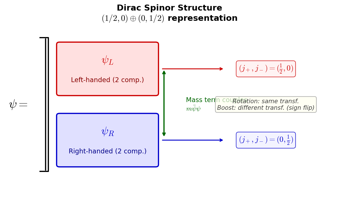
Fig. 5.1: Structure of the Dirac spinor. The 4-component Dirac spinor combines 2 components of the left-handed Weyl spinor \((1/2, 0)\) and 2 components of the right-handed Weyl spinor \((0, 1/2)\). The mass term \(m\bar{\psi}\psi\) couples the two.
✅ Comprehension Check: State one physical consequence of the Lorentz algebra decomposing into \(\mathfrak{su}(2) \oplus \mathfrak{su}(2)\).
Answer
Representations of the Lorentz group can be classified by pairs of independent \(\mathfrak{su}(2)\) spins \((j_+, j_-)\). This allows systematic classification of fields such as scalars \((0,0)\), Weyl spinors \((1/2, 0)\) and \((0, 1/2)\), Dirac spinors \((1/2, 0) \oplus (0, 1/2)\), and vectors \((1/2, 1/2)\).
5.3 The Dirac Field Lagrangian and Preparation for Canonical Quantization
🟡 Lina: Now let's prepare to quantize the Dirac field. As we learned in Ch. 3, the first step in field quantization is writing down the classical Lagrangian density.
🔵 Kai: For the scalar field, the approach was "choose a Lagrangian such that the Euler-Lagrange equation yields the Klein-Gordon equation." But the Dirac equation is a first-order differential equation for a 4-component spinor, so the form of the Lagrangian must be quite different.
🟡 Lina: Good intuition. The approach is the same—"choose a Lagrangian such that the Euler-Lagrange equation yields the Dirac equation." But as you note, because it's a first-order equation, the structure of the Lagrangian is quite different from the scalar field. The answer is:
🔵 Kai: What is \(\bar{\psi}\)? Is it different from \(\psi^\dagger\)?
🟡 Lina: Good question. \(\bar{\psi}\) is called the Dirac adjoint and is defined as
The reason we use \(\psi^\dagger \gamma^0\) rather than simply \(\psi^\dagger\) is that \(\bar{\psi}\psi\) is a Lorentz scalar (a quantity invariant under Lorentz transformations). \(\psi^\dagger \psi\) does not form a Lorentz scalar.
🔵 Kai: I understand that \(\psi^\dagger \psi\) doesn't form a Lorentz scalar, but why does inserting \(\gamma^0\) make it work? Does \(\gamma^0\) have some special property?
🟡 Lina: Good question. Under Lorentz transformations (rotations and boosts), the Dirac spinor transforms as \(\psi \to S\psi\), where \(S\) is a \(4 \times 4\) transformation matrix determined by which Lorentz transformation is being performed. For rotations, \(S\) is unitary (\(S^\dagger S = \mathbf{1}\)), but for boosts, it's non-unitary—meaning \(S^\dagger S \neq \mathbf{1}\). So under \(\psi \to S\psi\), we get \(\psi^\dagger \psi \to \psi^\dagger S^\dagger S \psi \neq \psi^\dagger \psi\), which is not invariant.
On the other hand, with \(\gamma^0\) inserted, \(\bar{\psi}\psi \to \psi^\dagger S^\dagger \gamma^0 S \psi\), and a property of the spinor representation gives \(S^\dagger \gamma^0 S = \gamma^0\). For now, please accept this relation—the derivation details are in Appendix B. Using this relation, \(\bar{\psi}\psi \to \psi^\dagger S^\dagger \gamma^0 S \psi = \psi^\dagger \gamma^0 \psi = \bar{\psi}\psi\), which is Lorentz invariant. So \(\gamma^0\) compensates for the non-unitarity of boosts.
⚪ Mei: I see—\(\psi^\dagger \psi\) breaks under boosts, but \(\psi^\dagger \gamma^0 \psi\) is kept invariant thanks to \(S^\dagger \gamma^0 S = \gamma^0\).
🟡 Lina: Exactly. Now let's verify that this Lagrangian really yields the Dirac equation. There's a technique here. Since \(\psi\) is a complex field, it has two independent degrees of freedom: real part \(\psi_{\mathrm{Re}}\) and imaginary part \(\psi_{\mathrm{Im}}\). In the variational principle, the basic approach is "write the Euler-Lagrange equation for each independent degree of freedom." Instead of varying with respect to \(\psi_{\mathrm{Re}}\) and \(\psi_{\mathrm{Im}}\), we can treat \(\psi\) and \(\bar{\psi} = \psi^\dagger \gamma^0\) (the Hermitian conjugate of \(\psi\) multiplied by \(\gamma^0\)) as independent variables, obtaining the same number of equations. This is just a change of variables without changing the physics—like using \(z = x + iy\), \(z^* = x - iy\) instead of \(x, y\) coordinates. Varying with respect to \(\bar{\psi}\) gives the Dirac equation \((i\not\!\partial - m)\psi = 0\), and varying with respect to \(\psi\) gives its conjugate equation. Writing the Euler-Lagrange equation with respect to \(\bar{\psi}\):
Looking at \(\mathcal{L} = \bar{\psi}(i\gamma^\mu \partial_\mu - m)\psi\), since \(\partial_\mu \bar{\psi}\) (the derivative of \(\bar{\psi}\)) doesn't appear anywhere, the second term is zero. For the first term, we "differentiate" \(\mathcal{L}\) with respect to \(\bar{\psi}\)—precisely, with respect to each spinor component \(\bar{\psi}_\alpha\) (\(\alpha = 1, 2, 3, 4\)). Since \(\mathcal{L} = \bar{\psi}(i\gamma^\mu \partial_\mu - m)\psi = \sum_{\alpha=1}^{4} \bar{\psi}_\alpha [(i\gamma^\mu \partial_\mu - m)\psi]_\alpha\) (where the index \(\alpha\) runs over the 4 spinor components) is linear in each \(\bar{\psi}_\alpha\) (appearing only to first power), differentiating with respect to \(\bar{\psi}_\alpha\) simply removes \(\bar{\psi}_\alpha\) and leaves the rest—just as differentiating \(y = ax\) with respect to \(x\) leaves \(a\):
This gives 4 equations for \(\alpha = 1, 2, 3, 4\), which can be written collectively as \((i\gamma^\mu \partial_\mu - m)\psi = 0\)—the Dirac equation itself.
🔵 Kai: Just varying with respect to \(\bar{\psi}\) directly produces the Dirac equation! The Lagrangian is cleverly designed.
Conjugate Momentum — A Major Difference from the Scalar Field
🟡 Lina: Next, let's compute the conjugate momentum needed for canonical quantization. The momentum conjugate to \(\psi\) is
Expanding \(\mathcal{L} = \bar{\psi}(i\gamma^\mu \partial_\mu - m)\psi\), the only term containing \(\dot{\psi} = \partial_0 \psi\) is the \(\mu = 0\) term: \(i\bar{\psi}\gamma^0 \partial_0 \psi\). This term is linear in \(\dot{\psi}\) (only appearing to first power), so "differentiating" with respect to \(\dot{\psi}\) means extracting the coefficient of \(\dot{\psi}\)—just as differentiating \(f = a\dot{\psi}\) with respect to \(\dot{\psi}\) leaves \(a\). Therefore
Substituting \(\bar{\psi} = \psi^\dagger \gamma^0\) gives \(\Pi = i\psi^\dagger (\gamma^0)^2 = i\psi^\dagger\). Here we used \((\gamma^0)^2 = \mathbf{1}\) (the result of setting \(\mu = \nu = 0\) in the Clifford algebra (5.1)).
🔵 Kai: Wait, the conjugate momentum is \(i\psi^\dagger\)? For the scalar field, it was \(\pi = \dot{\phi}\), an independent quantity from \(\phi\)...
🟡 Lina: Yes, this is a major feature of the Dirac field. Because the Dirac equation is first-order in time, specifying only \(\psi\) as an initial condition completely determines the time evolution. \(\dot{\psi}\) is not an independent degree of freedom. The conjugate momentum being expressible directly in terms of \(\psi^\dagger\) reflects this fact.
⚪ Mei: So for the scalar field, \(\phi\) and \(\dot{\phi}\) were two independent initial conditions, but for the Dirac field, \(\psi\) alone suffices. That's obvious in hindsight since it's a first-order equation.
Hamiltonian Density
🟡 Lina: Let's obtain the Hamiltonian density via the Legendre transformation:
Expanding the Lagrangian as \(\mathcal{L} = i\bar{\psi}\gamma^0\partial_0\psi + i\bar{\psi}\gamma^j\partial_j\psi - m\bar{\psi}\psi\), and noting \(\bar{\psi}\gamma^0 = \psi^\dagger(\gamma^0)^2 = \psi^\dagger\), the first term is \(i\psi^\dagger \dot{\psi}\). This is the same as \(\Pi\dot{\psi} = i\psi^\dagger \dot{\psi}\), so in \(\mathcal{H} = \Pi\dot{\psi} - \mathcal{L}\), the \(i\psi^\dagger\dot{\psi}\) terms cancel, giving
🔵 Kai: The time derivative term cancels, leaving only spatial derivatives and the mass term.
🟡 Lina: Right. Substituting \(\bar{\psi} = \psi^\dagger\gamma^0\) gives \(\bar{\psi}\gamma^j = \psi^\dagger\gamma^0\gamma^j\) and \(m\bar{\psi}\psi = m\psi^\dagger\gamma^0\psi\), so
Defining \(\boldsymbol{\gamma} \cdot \nabla \equiv \gamma^1\partial_1 + \gamma^2\partial_2 + \gamma^3\partial_3 = \gamma^j\partial_j\), both terms have \(\psi^\dagger\) (a \(1 \times 4\) row vector) on the far left and \(\psi\) (a \(4 \times 1\) column vector) on the far right, so we can collect the \(4 \times 4\) matrix sandwiched between them into parentheses:
Here we've simply collected the \(4 \times 4\) matrix sandwiched between \(\psi^\dagger\) (a \(1 \times 4\) row vector) and \(\psi\) (a \(4 \times 1\) column vector) into parentheses—it's the matrix product form \(\psi^\dagger M \psi\).
Alternatively, expanding the Dirac equation \((i\gamma^\mu\partial_\mu - m)\psi = 0\) gives \(i\gamma^0\partial_0\psi = -i\gamma^j\partial_j\psi + m\psi\). Multiplying from the left by \(\gamma^0\) (using \((\gamma^0)^2 = \mathbf{1}\)) gives \(i\partial_0\psi = (-i\gamma^0\boldsymbol{\gamma}\cdot\nabla + m\gamma^0)\psi\). This is exactly the content of the parentheses in equation (5.9), so for fields satisfying the equations of motion (this situation is called "on-shell"—when the field satisfies its equation of motion),
which is a simple expression. Since we'll use the Heisenberg picture for quantization, field operators satisfy the equations of motion (the Dirac equation)—the same structure as when the scalar field satisfied the Klein-Gordon equation in Ch. 4. So we can safely use this expression.
✅ Comprehension Check: State the essential difference between the conjugate momentum of the Dirac field and that of the scalar field.
Answer
For the scalar field, \(\pi = \dot{\phi}\), where \(\phi\) and \(\dot{\phi}\) are independent variables. For the Dirac field, \(\Pi = i\psi^\dagger\), meaning the conjugate momentum is directly expressible in terms of the complex conjugate of the field \(\psi\). This reflects the fact that the Dirac equation is first-order in time.
5.4 Attempting Quantization with Commutation Relations — And the Breakdown
🟡 Lina: Now, it's time to quantize. Following the same procedure as Ch. 4, we promote the field \(\psi\) and conjugate momentum \(\psi^\dagger\) to operators.
First, let's deliberately impose commutation relations just as we did for the scalar field. The reason I say "deliberately" is so you can experience that this is wrong.
🔵 Kai: We're doing the wrong thing first?
🟡 Lina: The best way to understand "why anticommutation relations are necessary" is to actually see "what breaks with commutation relations."
Mode Expansion
🟡 Lina: First, let's expand the field in plane wave solutions of the Dirac equation. The relativistic energy-momentum relation \(E^2 = |\boldsymbol{p}|^2 + m^2\) admits two solutions: \(E = +\sqrt{|\boldsymbol{p}|^2 + m^2}\) and \(E = -\sqrt{|\boldsymbol{p}|^2 + m^2}\). The Dirac equation also has these two types of solutions—positive-energy solutions \(u^s(\boldsymbol{p})e^{-ip \cdot x}\) (with \(p^0 = E_{\boldsymbol{p}} > 0\)) and negative-energy solutions \(v^s(\boldsymbol{p})e^{+ip \cdot x}\). The general solution is a superposition of these:
Here we adopt the integration measure convention \(\int \frac{d^3p}{(2\pi)^3}\) (in Ch. 4 we used \(\int \frac{d^3p}{(2\pi)^{3/2}}\), but the current convention makes the factors of \((2\pi)\) easier to organize when computing scattering amplitudes with interactions in later chapters, so from this chapter onward we unify to this convention. When citing results from Ch. 4, please be mindful of this convention difference). The convention difference only changes where factors of \((2\pi)\) appear, without affecting physical results (probabilities and cross sections). By analogy, it's like choosing to measure length in "meters" versus "centimeters"—the numbers change but the physics is the same. Specifically, in the Ch. 4 convention the right-hand side of commutation relations was \(\delta^{(3)}(\boldsymbol{p} - \boldsymbol{q})\), whereas in this chapter's convention it becomes \((2\pi)^3\delta^{(3)}(\boldsymbol{p} - \boldsymbol{q})\). Similarly, the normalization of one-particle states changes to \(\langle\boldsymbol{p}|\boldsymbol{q}\rangle = (2\pi)^3\delta^{(3)}(\boldsymbol{p} - \boldsymbol{q})\). This is merely the difference between absorbing the \((2\pi)^3\) from the integration measure into the operator normalization versus leaving it on the right-hand side of the (anti)commutation relations. Note that the \((2\pi)^3\) also appears on the right-hand side of the field (anti)commutation relations below, consistent with this convention change.
Taking the Hermitian conjugate of both sides of equation (5.11), operators become \(\hat{b}^s \to \hat{b}^{s\dagger}\), \(\hat{c}^{s\dagger} \to \hat{c}^s\), spinors become \(u^s \to u^{s\dagger}\), \(v^s \to v^{s\dagger}\), and exponentials have their signs flipped: \((e^{-ip\cdot x})^* = e^{+ip\cdot x}\), \((e^{+ip\cdot x})^* = e^{-ip\cdot x}\). Further multiplying from the right by \(\gamma^0\) gives \(u^{s\dagger}\gamma^0 = \bar{u}^s\), \(v^{s\dagger}\gamma^0 = \bar{v}^s\) (by the definition of the Dirac adjoint). The result is
Here:
- \(E_{\boldsymbol{p}} = \sqrt{|\boldsymbol{p}|^2 + m^2}\)
-
\(s = 1, 2\) labels spin degrees of freedom (up and down) Let me confirm the notation. \(p \cdot x \equiv p^\mu x_\mu = E_{\boldsymbol{p}}t - \boldsymbol{p}\cdot\boldsymbol{x}\) is the 4-vector inner product notation introduced in Ch. 4 (corresponding to the metric sign convention \((+,-,-,-)\) from Ch. 2). \(\not\!p \equiv \gamma^\mu p_\mu = \gamma^0 E_{\boldsymbol{p}} - \boldsymbol{\gamma}\cdot\boldsymbol{p}\) is the momentum version of the slash notation.
-
\(u^s(\boldsymbol{p})\): Positive-energy spinor—substituting the plane wave solution \(\psi = u\, e^{-ip \cdot x}\) into the Dirac equation, since \(\partial_\mu e^{-ip\cdot x} = -ip_\mu\, e^{-ip\cdot x}\), the Dirac equation becomes \((\not\!p - m)u\,e^{-ip\cdot x} = 0\), and dividing by \(e^{-ip\cdot x} \neq 0\):
This is the equation satisfied by \(u^s\). For each momentum \(\boldsymbol{p}\), there are 2 independent solutions \(u^1, u^2\) corresponding to the 2 spin degrees of freedom. The explicit form depends on the representation of the \(\gamma\) matrices, but for the current discussion it suffices to know that "there are two 4-component spinors satisfying \((\not\!p - m)u = 0\)." To build intuition, let's just look at the rest frame \(\boldsymbol{p} = \boldsymbol{0}\): then \(\not\!p = \gamma^0 m\), so the equation becomes \((\gamma^0 - 1)m\,u = 0\), i.e., \(\gamma^0 u = u\). In the chiral representation, \(\gamma^0\) is a matrix that swaps the upper and lower 2 components, so \(u^1\) and \(u^2\) are spinors with equal upper and lower 2 components. For the explicit form at general \(\boldsymbol{p}\), see Appendix B. - \(v^s(\boldsymbol{p})\): Negative-energy spinor (a historical name. As we'll see later, in quantum field theory \(\hat{c}^\dagger\) creates a positive-energy antiparticle, so "negative energy" is merely a classification of classical equation solutions).
An important convention to note: we keep $p^0 = E_{\boldsymbol{p}} > 0$ unchanged and put the sign in the exponential as $e^{+ip\cdot x}$. The reason is that in the mode expansion, the momentum integral runs from $-\infty$ to $+\infty$, so fixing $p^0 = E_{\boldsymbol{p}} > 0$ gives a cleaner integral structure.

The time dependence is $e^{+iE_{\boldsymbol{p}}t}$. Recall from quantum mechanics that the time dependence of a stationary state with energy $E$ is $e^{-iEt}$ (in natural units). Rewriting $e^{+iE_{\boldsymbol{p}}t} = e^{-i(-E_{\boldsymbol{p}})t}$, this formally corresponds to a solution with energy $-E_{\boldsymbol{p}}$—hence the name "negative-energy solution."

Let's derive the equation satisfied by $v^s$. Substituting $\psi = v\, e^{+ip \cdot x}$ into the Dirac equation $(i\gamma^\mu\partial_\mu - m)\psi = 0$: since $v$ is a constant spinor, the derivative acts only on $e^{+ip\cdot x}$, giving $\partial_\mu e^{+ip\cdot x} = (+ip_\mu)\,e^{+ip\cdot x}$. Substituting:
Here, the first \(i\) is the \(i\) already present in the Dirac equation operator \(i\gamma^\mu\partial_\mu\), and the \(i\) in \((+ip_\mu)\) came from the derivative. Multiplying the two \(i\)'s gives \(i \times i = i^2 = -1\). The remaining \(\gamma^\mu p_\mu\) is \(\not\!p\) in slash notation, so
The full Dirac equation is \((i\gamma^\mu\partial_\mu - m)\psi = 0\), so substituting \(\psi = v\,e^{+ip\cdot x}\) gives \((i\gamma^\mu\partial_\mu - m)(v\,e^{+ip\cdot x}) = 0\). The first term on the left is what we just computed: \(-\not\!p\, v\, e^{+ip\cdot x}\), and the second term is \(-m\,v\,e^{+ip\cdot x}\). Together: \((-\not\!p - m)v\,e^{+ip\cdot x} = 0\), multiplying both sides by \(-1\) gives \((\not\!p + m)v\,e^{+ip\cdot x} = 0\). Dividing by \(e^{+ip\cdot x} \neq 0\):
🔵 Kai: \(u\) satisfies \((\not\!p - m)u = 0\), and \(v\) satisfies \((\not\!p + m)v = 0\)—the sign of the mass term is opposite.
🟡 Lina: Exactly. These spinors satisfy orthogonality and completeness relations. I'll explain the details when we use them later, but let me state one important fact here: the 4 spinors \(u^1, u^2, v^1, v^2\) form a complete basis for 4-dimensional space. That is, any 4-component spinor can be written as a linear combination of these 4. The explicit forms of the completeness relations are
The right-hand sides are \(4 \times 4\) matrices because \(u\bar{u}\) is "column vector × row vector" which produces a matrix—for example, in the 2-component case, \(\begin{pmatrix} a \\ b \end{pmatrix}(c\ d) = \begin{pmatrix} ac & ad \\ bc & bd \end{pmatrix}\), and the same happens for 4 components. Why the right-hand side takes this particular form can be understood from the fact that \(u^s\) satisfies \((\not\!p - m)u^s = 0\)—\(\not\!p + m\) plays the role of a "projection operator onto the 2-dimensional subspace where \(u\) lives" (precisely, dividing by \(2m\) gives the projection operator \((\not\!p + m)/(2m)\)). Similarly, \(-(\not\!p - m)/(2m)\) is the projection operator onto the \(v\) subspace. Note that the sign of the mass term is opposite for \(u\bar{u}\) and \(v\bar{v}\) (\(+m\) and \(-m\)). This will be used repeatedly in later calculations.
Table 5.2: Operators appearing in the Dirac field mode expansion
| Operator | Role | Position in \(\hat{\psi}\) | Energy sign |
|---|---|---|---|
| \(\hat{b}^s_{\boldsymbol{p}}\) | Particle annihilation | Positive-energy term | \(e^{-ip\cdot x}\) |
| \(\hat{b}^{s\dagger}_{\boldsymbol{p}}\) | Particle creation | (in \(\hat{\bar{\psi}}\)) | \(e^{+ip\cdot x}\) |
| \(\hat{c}^s_{\boldsymbol{p}}\) | Antiparticle annihilation | (in \(\hat{\bar{\psi}}\)) | \(e^{-ip\cdot x}\) |
| \(\hat{c}^{s\dagger}_{\boldsymbol{p}}\) | Antiparticle creation | Negative-energy term | \(e^{+ip\cdot x}\) |
🔵 Kai: For the real scalar field there was only one set \(\hat{a}\) and \(\hat{a}^\dagger\), but now there are two sets \(\hat{b}\) and \(\hat{c}\). Why do the annihilation operator \(\hat{b}\) and creation operator \(\hat{c}^\dagger\) coexist within \(\hat{\psi}\)?
🟡 Lina: Good question. The Dirac field describes both particles and antiparticles, so two sets are needed. This is the same reason that the complex scalar field in Ch. 4 required two sets \(\hat{a}\) (particle) and \(\hat{b}\) (antiparticle). Having \(\hat{c}^\dagger\) (antiparticle creation operator) inside \(\hat{\psi}\) also has the same structure as the complex scalar field—the field operator either "annihilates a particle" or "creates an antiparticle."
Imposing Commutation Relations — An Ominous Sign
🟡 Lina: Now let's impose equal-time commutation relations just as for the scalar field. For the scalar field we had \([\hat{\phi}(\boldsymbol{x}), \hat{\pi}(\boldsymbol{y})] = i\delta^{(3)}(\boldsymbol{x} - \boldsymbol{y})\). For the Dirac field, since the conjugate momentum is \(\Pi_\alpha = i\psi^\dagger_\alpha\), substituting \(\hat{\Pi}_\beta = i\hat{\psi}^\dagger_\beta\) into the canonical commutation relation \([\hat{\psi}_\alpha(\boldsymbol{x}), \hat{\Pi}_\beta(\boldsymbol{y})] = i\delta_{\alpha\beta}\delta^{(3)}(\boldsymbol{x} - \boldsymbol{y})\) gives \([\hat{\psi}_\alpha, i\hat{\psi}^\dagger_\beta] = i\delta_{\alpha\beta}\delta^{(3)}\). The constant \(i\) can be pulled out of the commutator (\([A, cB] = c[A, B]\)), giving \(i[\hat{\psi}_\alpha, \hat{\psi}^\dagger_\beta] = i\delta_{\alpha\beta}\delta^{(3)}\), and dividing both sides by \(i\): \([\hat{\psi}_\alpha, \hat{\psi}^\dagger_\beta] = \delta_{\alpha\beta}\delta^{(3)}\). This is the commutation relation in position space. Note there's no \((2\pi)^3\) on the right side. Since the integration measure in the mode expansion is \(\int \frac{d^3p}{(2\pi)^3}\), translating the position-space \(\delta^{(3)}(\boldsymbol{x} - \boldsymbol{y})\) to momentum space via Fourier transform moves the \((2\pi)^3\) from the measure to the right-hand side of the commutation relation, giving the form \((2\pi)^3\delta^{(3)}(\boldsymbol{p} - \boldsymbol{q})\) (see equation (5.15)). So let's write the commutation relation between \(\hat{\psi}\) and \(\hat{\psi}^\dagger\):
Here \(\alpha, \beta = 1, 2, 3, 4\) are Dirac spinor components. Let's translate these field commutation relations into commutation relations for creation and annihilation operators using the mode expansion (5.11).
🟡 Lina: Substituting the mode expansion into the left side of equation (5.13), products of \(e^{\pm ip \cdot x}\) and \(e^{\pm iq \cdot y}\) appear. Using the spatial integral \(\int d^3x\, e^{i(\boldsymbol{p} - \boldsymbol{q})\cdot\boldsymbol{x}} = (2\pi)^3\delta^{(3)}(\boldsymbol{p} - \boldsymbol{q})\) to match momenta, the \(\hat{b}\) terms and \(\hat{c}\) terms separate. The key point is that \(\hat{c}^\dagger\) appears inside \(\hat{\psi}\), and \(\hat{c}\) appears inside \(\hat{\psi}^\dagger\) (look back at equation (5.11)). So when computing \([\hat{\psi}, \hat{\psi}^\dagger]\), the \(\hat{c}\)-related terms appear in the order \([\hat{c}^{s\dagger}_{\boldsymbol{p}},\, \hat{c}^s_{\boldsymbol{p}}]\)—with the creation operator first.
🔵 Kai: Ah, \([\hat{c}^\dagger, \hat{c}] = -[\hat{c}, \hat{c}^\dagger]\), so it has the opposite sign from the \(\hat{b}\) terms.
🟡 Lina: Exactly. Here we use "spinor orthogonality." This is the property that inner products of spinors with different spin states vanish—the same structure as \(\langle +|-\rangle = 0\) in quantum mechanics. Specifically, \(u^{r\dagger}(\boldsymbol{p})\,u^s(\boldsymbol{p}) \propto \delta^{rs}\) (zero for different spins \(r \neq s\)), and \(u^{r\dagger}(\boldsymbol{p})\,v^s(\boldsymbol{p}) = 0\) (positive-energy and negative-energy spinors are orthogonal). Using these to simplify, the left side of equation (5.13) takes the structure
🔵 Kai: I see that the second term appears in the order \([\hat{c}^{s\dagger}, \hat{c}^s]\). But why does this ultimately amount to attaching a minus sign to \([\hat{c}, \hat{c}^\dagger]\)?
🟡 Lina: To compare the right side \(\delta_{\alpha\beta}\,\delta^{(3)}(\boldsymbol{x} - \boldsymbol{y})\) with the left side, we need to bring both sides into the same form. Let me explain just the key point.
The left side has a \(\hat{b}\) term and a \(\hat{c}\) term. The \(\hat{b}\) term appears straightforwardly in the form \([\hat{b}, \hat{b}^\dagger]\). On the other hand, the \(\hat{c}\) term appears in the order \([\hat{c}^{s\dagger}, \hat{c}^s]\)—creation operator first—so converting to standard order gives \([\hat{c}^{s\dagger}, \hat{c}^s] = -[\hat{c}^s, \hat{c}^{s\dagger}]\)—a minus appears.
Meanwhile, we need to expand the right side \(\delta_{\alpha\beta}\,\delta^{(3)}(\boldsymbol{x} - \boldsymbol{y})\) in momentum space. Since we're working with \([\hat{\psi}, \hat{\psi}^\dagger]\), what appears in the mode expansion of \(\hat{\psi}^\dagger\) is \(u^{s\dagger}\) and \(v^{s\dagger}\) (Hermitian conjugates). These are different from \(\bar{u}^s = u^{s\dagger}\gamma^0\) (Dirac adjoint)—\(u\bar{u}\) is a Lorentz-covariant \(4 \times 4\) matrix, while \(uu^\dagger\) is simply the matrix made from column vector × row vector. We need to use the completeness relation to decompose the right side. I'll leave the technical details to exercise Problem M-1. Failure of Quantization via Commutation Relations, but the conclusion is: the 4 spinors \(u^1, u^2, v^1, v^2\) form a complete basis for 4-dimensional space (the analog of the completeness relation \(\sum_n |n\rangle\langle n| = \hat{1}\) from quantum mechanics). Using this completeness relation to decompose \(\delta_{\alpha\beta}\,\delta^{(3)}(\boldsymbol{x} - \boldsymbol{y})\) on the right side into the \(u\) contribution and the \(v\) contribution, both appear with positive coefficients. That is, the right side has the structure "\(u\) part = positive" + "\(v\) part = positive."
Matching the left and right sides term by term (from the completeness relations of \(u\) and \(v\), the right side \(\delta_{\alpha\beta}\delta^{(3)}\) decomposes into \(u\) and \(v\) contributions each with positive coefficients):
- \(\hat{b}\) term (corresponding to \(u\)): \([\hat{b}, \hat{b}^\dagger] = +\delta\) → consistent ✓
- \(\hat{c}\) term (corresponding to \(v\)): \(-[\hat{c}, \hat{c}^\dagger] = +\delta\) → requires \([\hat{c}, \hat{c}^\dagger] = -\delta\) ✗
This \(-\delta\) is the fatal minus sign. Summarizing the key point: in \(\hat{\psi}\), the positive-energy term contains the annihilation operator \(\hat{b}\), while the negative-energy term contains the creation operator \(\hat{c}^\dagger\). Because of this asymmetric structure, when taking the commutator, the \(\hat{c}\) terms appear in reverse order \([\hat{c}^\dagger, \hat{c}]\), which is the root cause of the minus sign. Technical details including the derivation of completeness relations are addressed in exercise Problem M-1. Failure of Quantization via Commutation Relations.
🔵 Kai: I see... so because \(\hat{c}^\dagger\) (a creation operator) is inside \(\hat{\psi}\), when computing \([\hat{\psi}, \hat{\psi}^\dagger]\) the \(\hat{c}\) terms appear in the order \(\hat{c}^\dagger\hat{c}\)—creation first. But why does the mode expansion have the annihilation operator \(\hat{b}\) in the positive-energy term and the creation operator \(\hat{c}^\dagger\) in the negative-energy term? Wouldn't the reverse work?
🟡 Lina: Good question. This is the unique choice that simultaneously satisfies both the condition "the vacuum is annihilated by annihilation operators" \(\hat{b}|0\rangle = \hat{c}|0\rangle = 0\) and the requirement that the field operator has the correct time dependence. The \(\hat{b}\) term has \(e^{-ip\cdot x}\) (positive frequency), and the \(\hat{c}^\dagger\) term has \(e^{+ip\cdot x}\) (negative frequency)—this ensures that \(\hat{\psi}\) satisfies the Dirac equation while making the vacuum the lowest-energy state. The result is:
🔵 Kai: Wait, there's a minus sign in front of \([\hat{c}, \hat{c}^\dagger]\)!
🟡 Lina: Yes. This is fatal. Let's see what physical problem this minus sign causes.
✅ Comprehension Check: What is the root cause of the minus sign appearing in \([\hat{c}, \hat{c}^\dagger]\) in equation (5.15b)?
Answer
Because the creation operator \(\hat{c}^\dagger\) appears in the negative-energy term of the mode expansion (5.11), computing \([\hat{\psi}, \hat{\psi}^\dagger]\) produces the \(\hat{c}\) terms in the order \([\hat{c}^{s\dagger}, \hat{c}^s] = -[\hat{c}^s, \hat{c}^{s\dagger}]\). Meanwhile, expanding the right-hand side \(\delta\) function using the spinor completeness relation shows the \(v\) contribution appears with a positive coefficient, so comparing both sides requires \([\hat{c}, \hat{c}^\dagger] = -\delta\).
🔵 Kai: Okay, I understand the structure. But what physical problem does this minus sign actually cause? If it's just a mathematical sign change, it might not be a big deal...
🟡 Lina: Good question. "Just a sign" turns out to be fatal. Let's see why.
Computing the Hamiltonian — Energy is Bottomless
🟡 Lina: Let's see what catastrophe this minus sign causes physically. We'll substitute the mode expansion into the Hamiltonian.
Substituting into \(\hat{H} = \int d^3x\, \hat{\psi}^\dagger\, i\partial_0\, \hat{\psi}\) and simplifying (the intermediate calculation is somewhat long, but there are 3 key points. First, when \(i\partial_0\) acts on the positive-energy solution \(e^{-ip\cdot x}\) it produces \(i \times (-iE_{\boldsymbol{p}}) = +E_{\boldsymbol{p}}\), and on the negative-energy solution \(e^{+ip\cdot x}\) it produces \(i \times (+iE_{\boldsymbol{p}}) = -E_{\boldsymbol{p}}\)—this \(-E_{\boldsymbol{p}}\) is the direct cause of the minus sign on the \(\hat{c}\) term in equation (5.16). Second, expanding the product \(\hat{\psi}^\dagger\) and \(\hat{\psi}\) produces 4 types of terms: \(\hat{b}^\dagger\hat{b}\), \(\hat{c}\hat{c}^\dagger\), \(\hat{b}^\dagger\hat{c}^\dagger\), \(\hat{c}\hat{b}\), but the cross terms (\(\hat{b}^\dagger\hat{c}^\dagger\) and \(\hat{c}\hat{b}\)) contain exponentials \(e^{\pm i(\boldsymbol{p}+\boldsymbol{q})\cdot\boldsymbol{x}}\) with different momenta, so they vanish upon spatial integration \(\int d^3x\) (spinor orthogonality \(u^\dagger v = 0\) is also used). Third, the surviving \(\hat{c}\hat{c}^\dagger\) ordering—\(\hat{c}\) from \(\hat{\psi}^\dagger\) multiplied by \(\hat{c}^\dagger\) from \(\hat{\psi}\), so the creation operator is on the right—this ordering matters when reordering in the next step. See exercise Problem M-1. Failure of Quantization via Commutation Relations for details):
🔵 Kai: There's a minus sign on the \(\hat{c}\hat{c}^\dagger\) term. Reordering using the commutation relation...
🟡 Lina: Using commutation relation (5.15b) to write \(\hat{c}\hat{c}^\dagger = \hat{c}^\dagger\hat{c} + [\hat{c}, \hat{c}^\dagger]\):
Since \([\hat{c}, \hat{c}^\dagger] = -(2\pi)^3\delta^{(3)}(\boldsymbol{0})\):
Removing the infinite constant by normal ordering as with the scalar field, the Hamiltonian becomes
🔵 Kai: There's a minus in front of \(\hat{c}^\dagger\hat{c}\)... that means every time we create an antiparticle, the energy decreases!?
🟡 Lina: Exactly. Each time \(\hat{c}^{s\dagger}_{\boldsymbol{p}}\) creates an antiparticle, the energy changes by \(-E_{\boldsymbol{p}}\). Since we can create arbitrarily many antiparticles, the energy can decrease without limit—it becomes unbounded below.
⚪ Mei: So there's no stable vacuum state. We can make states with arbitrarily low energy. This is physically unacceptable.
🟡 Lina: Precisely. Quantizing the Dirac field with commutation relations leads to a breakdown of the theory. That's why I said "let's deliberately experience the mistake." The difference is visually compared in Fig. 5.2 "Comparison of energy spectra with commutation vs" (the result using anticommutation relations is derived in the next section, but I'm showing the conclusion ahead of time for comparison).
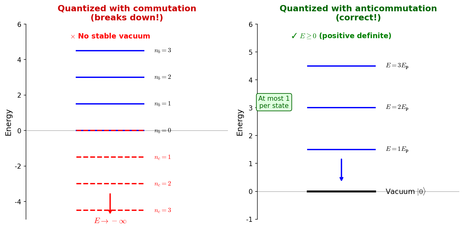
Fig. 5.2: Comparison of energy spectra with commutation vs. anticommutation relations. With commutation relations, each antiparticle creation lowers the energy \(E \to -\infty\) (no stable vacuum). With anticommutation relations, energy is positive-definite (derived in 5.5 "Introducing Anticommutation Relations — The Prescription That Saves Everything"), and each state can hold at most 1 particle (derived in 5.6 "The Pauli Exclusion Principle — A Gift from Anticommutation Relations").
✅ Comprehension Check: Referring to equation (5.17), explain why the Hamiltonian energy becomes unbounded below when the Dirac field is quantized with commutation relations. Include what it means that "no stable vacuum state exists."
Answer
In equation (5.17), the minus sign in front of \(\hat{c}^{s\dagger}_{\boldsymbol{p}}\hat{c}^s_{\boldsymbol{p}}\) means that as the antiparticle number operator \(\hat{N}_c = \hat{c}^\dagger\hat{c}\) increases, the energy decreases. With commutation relations, the eigenvalues of \(\hat{N}_c\) are \(0, 1, 2, \ldots\) with no upper limit, so the energy can decrease to \(-\infty\). Therefore, no lowest-energy state (vacuum) beyond which energy cannot be further lowered can be defined, and no stable vacuum exists.
5.5 Introducing Anticommutation Relations — The Prescription That Saves Everything
🟡 Lina: Commutation relations have failed. So what should we do? The answer is—impose anticommutation relations instead of commutation relations.
Here \(\{A, B\} \equiv AB + BA\) is the anticommutator.
🔵 Kai: Just changing the commutator \([A, B] = AB - BA\) from minus to plus? Can such a simple change really fix the minus sign problem with \([\hat{c}^\dagger, \hat{c}]\)?
🟡 Lina: It's just a single sign change, but everything changes. Let's see how. Translating the field anticommutation relations (5.18) into the mode expansion: the structure of the calculation is exactly the same as for commutation relations (equation (5.13) → (5.15a,b))—the only difference is that \([A, B] = AB - BA\) becomes \(\{A, B\} = AB + BA\). The \(v\) terms again appear in the order \(\{\hat{c}^{s\dagger}, \hat{c}^s\}\), but the anticommutator is symmetric \(\{A, B\} = \{B, A\}\), so \(\{\hat{c}^{s\dagger}, \hat{c}^s\} = \{\hat{c}^s, \hat{c}^{s\dagger}\}\)—no minus sign appears from reordering, unlike with commutation relations. The results are:
All others vanish:
⚪ Mei: The anticommutation relation for \(\hat{c}\) in (5.20b) has no minus sign! The ominous minus that was in equation (5.15b) with commutation relations has disappeared!
🟡 Lina: Exactly. Let me explain why the minus disappears by contrasting with the commutation relation case.
With commutation relations: computing \([\hat{\psi}, \hat{\psi}^\dagger]\), the \(v\) terms appeared in the order \([\hat{c}^{s\dagger}, \hat{c}^s]\). Converting to standard order: \([\hat{c}^{s\dagger}, \hat{c}^s] = -[\hat{c}^s, \hat{c}^{s\dagger}]\)—a minus appears.
With anticommutation relations: computing \(\{\hat{\psi}, \hat{\psi}^\dagger\}\), the \(v\) terms similarly appear in the order \(\{\hat{c}^{s\dagger}, \hat{c}^s\}\). But the anticommutator is symmetric by definition \(\{A, B\} = AB + BA\), so \(\{\hat{c}^{s\dagger}, \hat{c}^s\} = \{\hat{c}^s, \hat{c}^{s\dagger}\}\)—no minus appears from reordering.
🔵 Kai: I see! The commutator is antisymmetric \([A, B] = -[B, A]\) so reordering produces a minus, but the anticommutator is symmetric \(\{A, B\} = \{B, A\}\) so no minus appears—that's the decisive difference.
🟡 Lina: This difference is decisive. That's why even for the \(v\) terms, \(\{\hat{c}, \hat{c}^\dagger\}\) appears directly with a positive coefficient, and no minus sign arises in equation (5.20b). Let's see concretely how this reflects in the Hamiltonian in the next recalculation.
Recalculating the Hamiltonian — Energy Becomes Positive-Definite
🟡 Lina: Let's recalculate the Hamiltonian. Equation (5.16):
is unchanged. What differs is that we now use the anticommutation relation to reorder \(\hat{c}\hat{c}^\dagger\). With commutation relations, we used \([A, B] = AB - BA\) rearranged as \(AB = BA + [A, B]\) (connected by \(+\)), but with anticommutation relations, \(\{A, B\} = AB + BA\) rearranges to \(AB = -BA + \{A, B\}\) (connected by \(-\))—this sign difference is decisive:
Since \(\{\hat{c}, \hat{c}^\dagger\} = (2\pi)^3\delta^{(3)}(\boldsymbol{0})\) (positive this time!):
🔵 Kai: The original minus and the reordering minus cancel each other out, making the sign in front of \(\hat{c}^\dagger\hat{c}\) positive!
🟡 Lina: The \((2\pi)^3\delta^{(3)}(\boldsymbol{0})\) is a constant that diverges in the limit \(V \to \infty\), just as in Ch. 4. Normal ordering for fermions, like for bosons, is the operation of "placing creation operators to the left of annihilation operators and discarding the c-numbers that arise in the process," but with one difference—each time fermion operators are interchanged, a minus sign is attached (reflecting the anticommutation relations). In the present case, we're just reordering \(\hat{c}\hat{c}^\dagger\) to \(\hat{c}^\dagger\hat{c}\), so discarding the constant term gives
⚪ Mei: The minus has become a plus! Both particles and antiparticles contribute positively to the energy!
🔵 Kai: The right side of Fig. 5.2 "Comparison of energy spectra with commutation vs" showing "energy is positive-definite with anticommutation relations" is exactly this equation (5.21). But wait—removing the infinite constant by normal ordering is the same prescription as for bosons. Can it be justified the same way for fermions?
🟡 Lina: Good question. The physical justification for normal ordering is the same as for bosons—the prescription of "defining the vacuum energy as zero." Since only energy differences are observable, adding or subtracting a constant doesn't change the physics. The same logic applies for fermions.
🔵 Kai: I see—"the absolute zero point of energy can't be measured," so we take the vacuum as the reference and count only differences from there—same reasoning for both bosons and fermions.
🟡 Lina: Now, since \(E_{\boldsymbol{p}} > 0\) and the eigenvalues of number operators \(\hat{b}^\dagger\hat{b}\) and \(\hat{c}^\dagger\hat{c}\) are non-negative, the Hamiltonian is positive-definite. A stable vacuum \(|0\rangle\) (with \(\hat{b}|0\rangle = \hat{c}|0\rangle = 0\)) exists. To summarize what happened: when reordering \(-\hat{c}\hat{c}^\dagger\) in equation (5.16), the initial minus in the anticommutation formula \(AB = -BA + \{A, B\}\) cancelled the pre-existing minus, ultimately giving a plus—"minus × minus = plus" is the essence.
⚪ Mei: Comparing equations (5.17) and (5.21), the only difference is the sign in front of \(\hat{c}^\dagger\hat{c}\). It was minus with commutation relations and became plus with anticommutation relations—a single sign choice changes everything.
🔵 Kai: But why did nature "choose anticommutation relations"? Is it something we can freely decide, commutation vs. anticommutation? Or is there a deeper reason?
🟡 Lina: A very deep question. "Why must spin \(1/2\) use anticommutation relations?"—the answer will be revealed in the spin-statistics theorem in 5.8 "The Spin-Statistics Theorem — Why Fermions Anticommute". At this stage, we only have the conclusion by elimination that "commutation relations break things, so anticommutation relations are necessary," but there's actually a more fundamental reason—Lorentz invariance and causality—that connects spin and statistics. That's a treat for later.
🔵 Kai: So there's evidence that it's not just "elimination" but "necessity." Looking forward to it.
🟡 Lina: First let's see the consequences of anticommutation relations. How occupation numbers differ between commutation and anticommutation relations is previewed in Fig. 5.3 "Comparison of occupation numbers between commutation and anticommutation relations". Why "at most 1 per state" will be rigorously derived from the anticommutation relations in the next section.
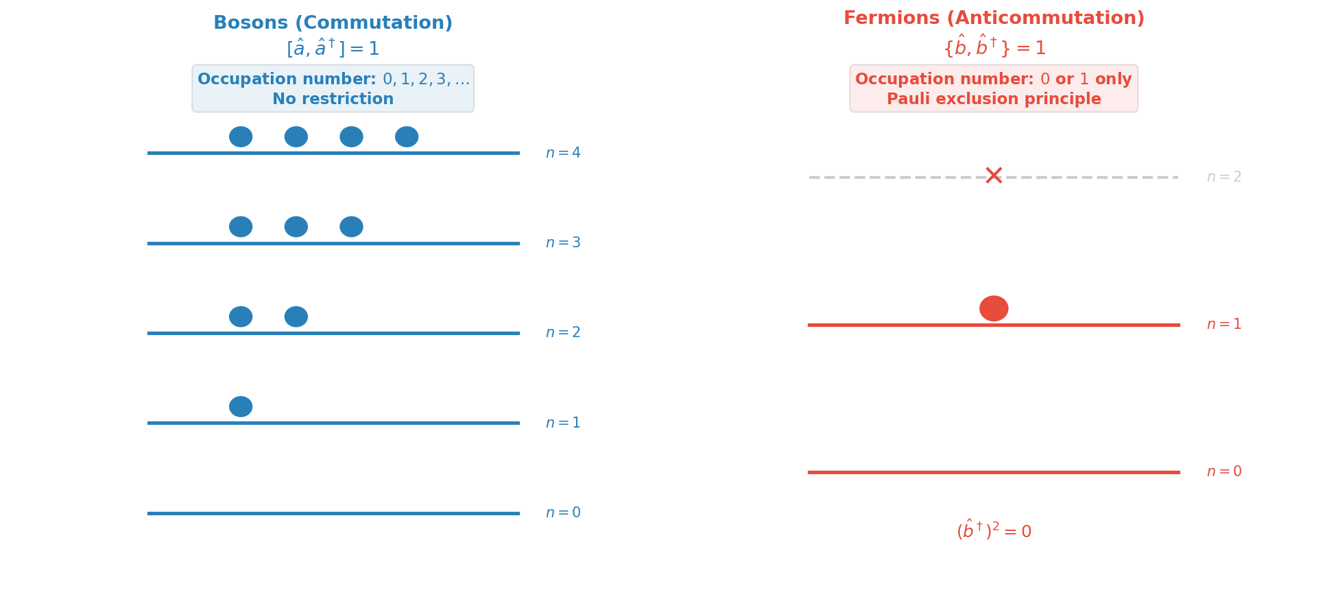
Fig. 5.3: Comparison of occupation numbers between commutation and anticommutation relations. For bosons (commutation relations), there's no limit on occupation number, but for fermions (anticommutation relations), each state can hold at most 1 particle (shown in detail in 5.6 "The Pauli Exclusion Principle — A Gift from Anticommutation Relations").
✅ Comprehension Check: Using the anticommutation relation \(\{\hat{c}, \hat{c}^\dagger\} = 1\) (discrete case), express \(\hat{c}\hat{c}^\dagger\) in terms of \(\hat{c}^\dagger\hat{c}\). Compare with the commutation relation \([\hat{c}, \hat{c}^\dagger] = -1\) case.
Answer
Anticommutation relation: \(\hat{c}\hat{c}^\dagger = 1 - \hat{c}^\dagger\hat{c}\). Therefore \(-\hat{c}\hat{c}^\dagger = -1 + \hat{c}^\dagger\hat{c}\) (after normal ordering: \(+\hat{c}^\dagger\hat{c}\)). Commutation relation: \(\hat{c}\hat{c}^\dagger = -1 + \hat{c}^\dagger\hat{c}\). Therefore \(-\hat{c}\hat{c}^\dagger = 1 - \hat{c}^\dagger\hat{c}\) (after normal ordering: \(-\hat{c}^\dagger\hat{c}\)). With anticommutation relations the energy contribution is positive; with commutation relations it's negative.
📝 Exercises:
- Comparison of Dirac field Hamiltonian with commutation vs. anticommutation relations → Problem M-1. Failure of Quantization via Commutation Relations
5.6 The Pauli Exclusion Principle — A Gift from Anticommutation Relations
🟡 Lina: Anticommutation relations have another crucial physical consequence. From equation (5.20c):
That is,
🔵 Kai: The square of the creation operator is zero! That means... if you try to put 2 particles into the same quantum state, the state becomes zero?
🟡 Lina: Exactly!
You cannot create 2 particles with the same momentum \(\boldsymbol{p}\) and same spin \(s\). This is the Pauli exclusion principle.
⚪ Mei: If you can't put in more than 2, there should also be an upper limit on the eigenvalues of the number operator \(\hat{N} = \hat{b}^\dagger\hat{b}\).
🟡 Lina: Right. Let's verify. \(\hat{N}^2 = \hat{b}^\dagger\hat{b}\hat{b}^\dagger\hat{b}\), and using the anticommutation relation \(\hat{b}\hat{b}^\dagger = 1 - \hat{b}^\dagger\hat{b}\): \(\hat{N}^2 = \hat{b}^\dagger(1 - \hat{b}^\dagger\hat{b})\hat{b} = \hat{b}^\dagger\hat{b} - (\hat{b}^\dagger)^2\hat{b}^2 = \hat{N} - 0 = \hat{N}\). The eigenvalues satisfying \(\hat{N}^2 = \hat{N}\) are only \(0\) or \(1\).
⚪ Mei: If the eigenvalue is \(n\), then \(n^2 = n\), so \(n(n-1) = 0\), giving \(n = 0\) or \(n = 1\). The exclusion principle emerges cleanly.
🔵 Kai: It's like a bit—only two choices, ON or OFF!
🟡 Lina: Perfect. Each quantum state can hold at most 1 particle—this is the essence of fermions. See Fig. 5.4 "Comparison of bosonic and fermionic Fock space structures" for the structural difference between bosonic and fermionic Fock spaces.
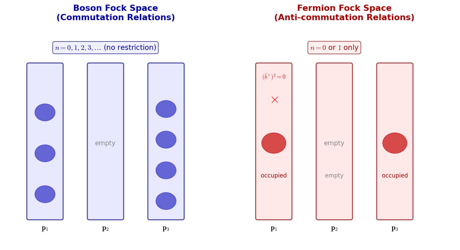
Fig. 5.4: Comparison of bosonic and fermionic Fock space structures. For bosons, any number of particles can occupy each quantum state, but for fermions, \((\hat{b}^\dagger)^2 = 0\) limits each state to at most 1 particle.
✅ Comprehension Check: From the anticommutation relation \(\{\hat{b}^{s\dagger}_{\boldsymbol{p}}, \hat{b}^{s\dagger}_{\boldsymbol{p}}\} = 0\), show that the eigenvalues of the number operator \(\hat{N} = \hat{b}^\dagger \hat{b}\) are only \(0\) and \(1\).
Answer
\(\hat{N}^2 = \hat{b}^\dagger \hat{b} \hat{b}^\dagger \hat{b}\), substituting the anticommutation relation \(\hat{b}\hat{b}^\dagger = 1 - \hat{b}^\dagger\hat{b}\) gives \(\hat{N}^2 = \hat{b}^\dagger(1 - \hat{b}^\dagger\hat{b})\hat{b} = \hat{b}^\dagger\hat{b} - (\hat{b}^\dagger)^2\hat{b}^2 = \hat{N} - 0 = \hat{N}\). The eigenvalues satisfying \(\hat{N}^2 = \hat{N}\) are \(n(n-1) = 0\), giving only \(n = 0\) or \(n = 1\).
Table 5.3: Comparison of quantization conditions for bosons and fermions
| Bosons (commutation relations) | Fermions (anticommutation relations) | |
|---|---|---|
| Quantization condition | \([\hat{a}, \hat{a}^\dagger] = 1\) | \(\{\hat{b}, \hat{b}^\dagger\} = 1\) |
| \((\hat{a}^\dagger)^2\) | \(\neq 0\) (can create any number) | \(= 0\) (cannot create more than 1) |
| Range of occupation number | \(0, 1, 2, 3, \ldots\) | \(0\) or \(1\) only |
| Statistics | Bose-Einstein statistics | Fermi-Dirac statistics |
🔵 Kai: In quantum mechanics, I was taught "the Pauli exclusion principle is assumed as an experimental fact," but in quantum field theory it's derived from anticommutation relations! But does that mean the exclusion principle in quantum mechanics was "something that could actually be proven but was assumed as an axiom"?
🟡 Lina: Good question. Within the framework of non-relativistic quantum mechanics alone, the exclusion principle cannot be derived. It can only be derived by combining relativity (Lorentz invariance) with quantum field theory. So assuming it as an axiom within quantum mechanics was the correct approach given the limitations of the theory at that time. This is the power of quantum field theory—the Pauli exclusion principle is not an axiom handed down from above, but an unavoidable consequence of the structure of relativistic field theory.
🔵 Kai: So quantum mechanics alone couldn't answer "why" the exclusion principle holds.
🟡 Lina: That's right. If these requirements themselves could be derived from an even deeper principle, then the next "why" might become visible—that remains an open question.
📝 Exercises:
- Derivation of the Pauli exclusion principle from anticommutation relations → Problem M-2. Derivation of the Pauli Exclusion Principle
5.7 Fermionic Fock Space and Antiparticles
🟡 Lina: Let's organize the structure of the fermionic Fock space.
Vacuum State
The vacuum contains neither particles nor antiparticles.
One-Particle States
\(\hat{b}^\dagger\) creates a particle (e.g., electron \(e^-\)), and \(\hat{c}^\dagger\) creates an antiparticle (e.g., positron \(e^+\)).
🔵 Kai: The positron was predicted by Dirac in 1928 and discovered by Anderson in cosmic rays in 1932, right?
🟡 Lina: Yes. Reinterpreting negative-energy solutions of the Dirac equation as "positive-energy solutions for antiparticles" is the modern understanding. In quantum field theory, \(\hat{c}^\dagger\) creates antiparticles with positive energy, so the old picture of a "negative-energy sea" is unnecessary (the two pictures are compared in Fig. 5.5 "Dirac sea and modern vacuum picture").
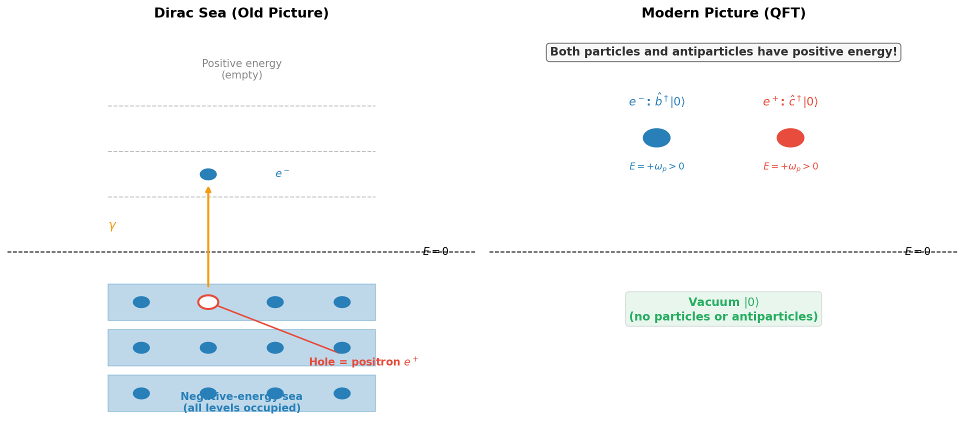
Fig. 5.5: Dirac sea and modern vacuum picture. Left: the old Dirac sea picture (all negative-energy levels are occupied, and holes are positrons). Right: the modern quantum field theory picture (particles and antiparticles are both created with positive energy from the vacuum).
✅ Comprehension Check: How does the interpretation of antiparticles in quantum field theory differ from Dirac's "negative-energy sea" picture?
Answer
In the Dirac sea picture, all negative-energy levels are occupied by electrons, and "holes" in this sea are observed as positrons. In quantum field theory, the antiparticle creation operator \(\hat{c}^\dagger\) directly creates antiparticles with positive energy from the vacuum, making the concept of a negative-energy sea unnecessary.
Many-Particle States and Antisymmetry
🟡 Lina: Let's consider a 2-particle state. Creating 2 electrons with different quantum numbers \((\boldsymbol{p}_1, s_1)\) and \((\boldsymbol{p}_2, s_2)\):
From the anticommutation relation \(\{\hat{b}^{s_1\dagger}_{\boldsymbol{p}_1}, \hat{b}^{s_2\dagger}_{\boldsymbol{p}_2}\} = 0\):
⚪ Mei: Exchanging two particles gives a minus sign to the state—the antisymmetry of the wave function. The many-body fermion wave function \(\Psi(1, 2) = -\Psi(2, 1)\) that we learned in quantum mechanics automatically emerges from anticommutation relations in quantum field theory.
🟡 Lina: And of course, if \(\boldsymbol{p}_1 = \boldsymbol{p}_2\) and \(s_1 = s_2\), then \((\hat{b}^{s\dagger}_{\boldsymbol{p}})^2|0\rangle = 0\)—the Pauli exclusion principle.
Charge Conservation
🟡 Lina: From Noether's theorem (Ch. 3), the conserved charge corresponding to the \(U(1)\) symmetry \(\psi \to e^{i\alpha}\psi\) of the Dirac field is
🔵 Kai: It's the number of particles minus the number of antiparticles! For electrons \(Q = -e\) and for positrons \(Q = +e\), so \(\hat{b}^\dagger\) creates charge \(-e\) and \(\hat{c}^\dagger\) creates charge \(+e\).
🟡 Lina: Exactly. Particles and antiparticles have the same mass and same spin, but opposite signs of charge (and other additive quantum numbers).
✅ Comprehension Check: Explain how the conserved charge \(\hat{Q}\) (equation (5.26)) assigns opposite-sign charges to particles and antiparticles.
Answer
Since \(\hat{Q} = \sum_s \int \frac{d^3p}{(2\pi)^3}[\hat{b}^{s\dagger}\hat{b}^s - \hat{c}^{s\dagger}\hat{c}^s]\), particles (created by \(\hat{b}^\dagger\)) contribute \(+1\) to \(\hat{Q}\), and antiparticles (created by \(\hat{c}^\dagger\)) contribute \(-1\). If the electron's charge is \(-e\), then \(\hat{b}^\dagger\) creates a particle with charge \(-e\), and \(\hat{c}^\dagger\) creates an antiparticle with charge \(+e\).
✅ Comprehension Check: From the anticommutation relation \(\{\hat{b}^{s_1\dagger}_{\boldsymbol{p}_1}, \hat{b}^{s_2\dagger}_{\boldsymbol{p}_2}\} = 0\), derive the antisymmetry of the 2-fermion state.
Answer
From \(\hat{b}^{s_1\dagger}_{\boldsymbol{p}_1}\hat{b}^{s_2\dagger}_{\boldsymbol{p}_2} + \hat{b}^{s_2\dagger}_{\boldsymbol{p}_2}\hat{b}^{s_1\dagger}_{\boldsymbol{p}_1} = 0\), we get \(\hat{b}^{s_1\dagger}_{\boldsymbol{p}_1}\hat{b}^{s_2\dagger}_{\boldsymbol{p}_2}|0\rangle = -\hat{b}^{s_2\dagger}_{\boldsymbol{p}_2}\hat{b}^{s_1\dagger}_{\boldsymbol{p}_1}|0\rangle\). Exchanging particles 1 and 2 gives a minus sign to the state.
5.8 The Spin-Statistics Theorem — Why Fermions Anticommute
🟡 Lina: So far we've seen that "quantizing the Dirac field with commutation relations makes the energy break down, while anticommutation relations make it positive-definite." But there's a deeper question. Why are spin-\(1/2\) particles quantized with anticommutation relations, and spin-\(0\) particles with commutation relations?
🔵 Kai: Is that just a coincidence?
🟡 Lina: It's not a coincidence. Within the framework of relativistic quantum field theory, the following theorem can be proven:
Spin-statistics theorem: - Fields with integer spin (\(s = 0, 1, 2, \ldots\)) are quantized with commutation relations → bosons - Fields with half-integer spin (\(s = 1/2, 3/2, \ldots\)) are quantized with anticommutation relations → fermions
🔵 Kai: How is this proven?
🟡 Lina: A completely rigorous proof is mathematically sophisticated, but the physical motivation can be understood from 3 independent arguments.
Argument 1: Breakdown of the "Wrong" Combination
🟡 Lina: This is exactly a generalization of what we just did.
- Quantizing the Dirac field (spin \(1/2\)) with commutation relations → energy becomes unbounded below (as we just saw)
- Quantizing the scalar field (spin \(0\)) with anticommutation relations → causality is violated (the anticommutator of the field at two spacelike-separated points doesn't vanish, producing correlations faster than light). This can be verified in an exercise (@exercise: Scalar field anticommutation relations and violation of causality → Problem B-9. Anticommutation Relations for a Scalar Field and Violation of Causality).
So choosing the "wrong" combination produces physically unacceptable consequences.
⚪ Mei: Trying the "wrong" one breaks either energy or causality—the correct combination is uniquely determined by elimination.
Argument 2: Causality (Microcausality Condition)
🟡 Lina: In relativity, information cannot propagate faster than light. In quantum field theory, this is expressed as:
At two spacelike-separated points \((x - y)^2 < 0\), the commutator of observables must vanish.
For bosonic fields, the field itself is a (building block of) observables, so \([\hat{\phi}(x), \hat{\phi}(y)] = 0\) is required. For fermionic fields, observables are bilinear forms like \(\bar{\psi}\psi\)—products of an even number of fermion fields. Using anticommutation relations, it can be shown that the commutator of products of even numbers of fields vanishes in the spacelike region. Intuitively, when computing the commutator of \(\bar{\psi}(x)\psi(x)\) and \(\bar{\psi}(y)\psi(y)\), using anticommutation relations to rearrange the ordering of fermion fields shows that the commutator of products of even numbers of fields reduces to the same structure as bosonic field commutators—which vanish in the spacelike region.
🔵 Kai: So the fermion field itself isn't an observable, meaning it doesn't matter if \(\{\hat{\psi}(x), \hat{\psi}(y)\}\) isn't zero?
🟡 Lina: Exactly. Physical observables are products of even numbers like \(\bar{\psi}\psi\), so as long as their commutator vanishes, causality is preserved.
Argument 3: Path Dependence of Particle Exchange
🟡 Lina: There's another intuitive argument. Consider particle exchange as "one particle going halfway around the other."
When moving a particle spatially (rotating the orbital part), in relativistic field theory the particle's internal degrees of freedom (spin) are also affected by the same rotation—this is a consequence of the field belonging to a specific representation of the Lorentz group. Intuitively, "picking up a particle and moving it halfway around" corresponds to rotating the particle's own orientation (spin) as well. Imagine carrying a globe while walking—the globe's orientation changes together with you.
🔵 Kai: Why are "rotating the orbit" and "rotating the spin" linked?
🟡 Lina: In non-relativistic quantum mechanics, orbital angular momentum and spin could be treated independently. But in relativistic field theory, things are different. A field has a "value" at each point in space, and that value itself transforms as a spinor or vector. For example, think of the electric field vector \(\boldsymbol{E}\). If you rotate the coordinate system by \(\pi\), \(E_x\) and \(E_y\) mix, right?
⚪ Mei: So in field theory, "which point's value we look at" and "how components mix at that point" are inseparable.
🟡 Lina: Exactly. Mathematically, rotating a spin-\(s\) field about the \(z\)-axis by angle \(\theta\) applies the rotation operator \(e^{-iJ_z\theta}\). So the "orbital rotation angle" and the "spin rotation angle" are the same \(\theta\).
Now let's think concretely about the exchange operation for 2 particles. This isn't a rigorous proof but an intuitive argument that captures the essence. When exchanging two identical particles with a fixed center of mass, the relative position vector \(\boldsymbol{r} = \boldsymbol{x}_1 - \boldsymbol{x}_2\) changes to \(\boldsymbol{r} \to -\boldsymbol{r}\). This can be viewed as a rotation by angle \(\pi\) in the plane containing \(\boldsymbol{r}\) (in 3 dimensions, \(\boldsymbol{r} \to -\boldsymbol{r}\) is an inversion, but tracking the exchange path continuously, it can be realized as a \(\pi\) rotation in some plane).
The important point here is that each particle individually rotates by \(\pi\) around the midpoint. Visualize this concretely—particle 1 is to the right of the origin, particle 2 to the left (since they're identical particles with equal mass, the center of mass is exactly in the middle). To exchange them, move particle 1 through the upper semicircle to the left, and particle 2 through the lower semicircle to the right. It's like both ends of a balance making a half-turn—each one goes halfway (\(\pi\)) around the origin, right?
🔵 Kai: I see, so exchange = each particle goes halfway (\(\pi\) rotation).
🟡 Lina: Right. In relativistic field theory, rotating a particle spatially by \(\pi\) also applies the same \(\pi\) rotation to that particle's spin degrees of freedom (the "field components mix under rotation" property explained earlier). Let me supplement why the phase is attached "to each particle independently." The rotation operator for a 2-particle system is written as a tensor product \(e^{-iJ_z^{(1)}\theta} \otimes e^{-iJ_z^{(2)}\theta}\)—since particle 1's spin and particle 2's spin are independent degrees of freedom, the rotation acts on each independently. So each particle's spin component (focusing on \(m = s\)) picks up a phase \(e^{-is\pi}\), and since the 2-particle state is written as a tensor product \(|\text{particle 1}\rangle \otimes |\text{particle 2}\rangle\), the two phase factors multiply:
Let's compute concretely:
- \(s = 0\) (scalar): \(e^{0} = +1\)
- \(s = 1/2\) (Dirac): \(e^{-i\pi} = \cos\pi + i\sin\pi = -1\)
- \(s = 1\) (vector): \(e^{-2i\pi} = \cos 2\pi + i\sin 2\pi = +1\)
In general:
- \(s\) integer: \(e^{-2is\pi} = +1\) → bosons
- \(s\) half-integer: \(e^{-2is\pi} = -1\) → fermions
🔵 Kai: The property that a spinor picks up a sign flip under \(360°\) rotation is what matters here! The "\(720°\) to return to the original" from 5.2 "Spinor Representations of the Lorentz Group — Spinors Are Not Vectors" was precisely the origin of Fermi statistics.
🟡 Lina: Exactly. Looking back at the 3 arguments: Argument 1 is "the wrong combination breaks either energy or causality," Argument 2 is "causality requires fermionic fields to have anticommutation relations," Argument 3 is "the phase of particle exchange is determined by spin"—all three independent angles converge on the same conclusion.
⚪ Mei: Summarizing Argument 3: each particle picks up a phase \(e^{-is\pi}\) from the \(\pi\) rotation, and for 2 particles it becomes \(e^{-2is\pi}\)—for half-integer spin this gives \(-1\) (antisymmetric), and for integer spin \(+1\) (symmetric).
🟡 Lina: Right. All three arguments converge on the same conclusion that "spin determines statistics"—this is the core of the spin-statistics theorem.
The connection between spin and statistics is one of the deepest consequences of relativistic quantum field theory. It cannot be derived from non-relativistic quantum mechanics alone. The whole picture is summarized in Fig. 5.6 "Conceptual diagram of the spin-statistics theorem".
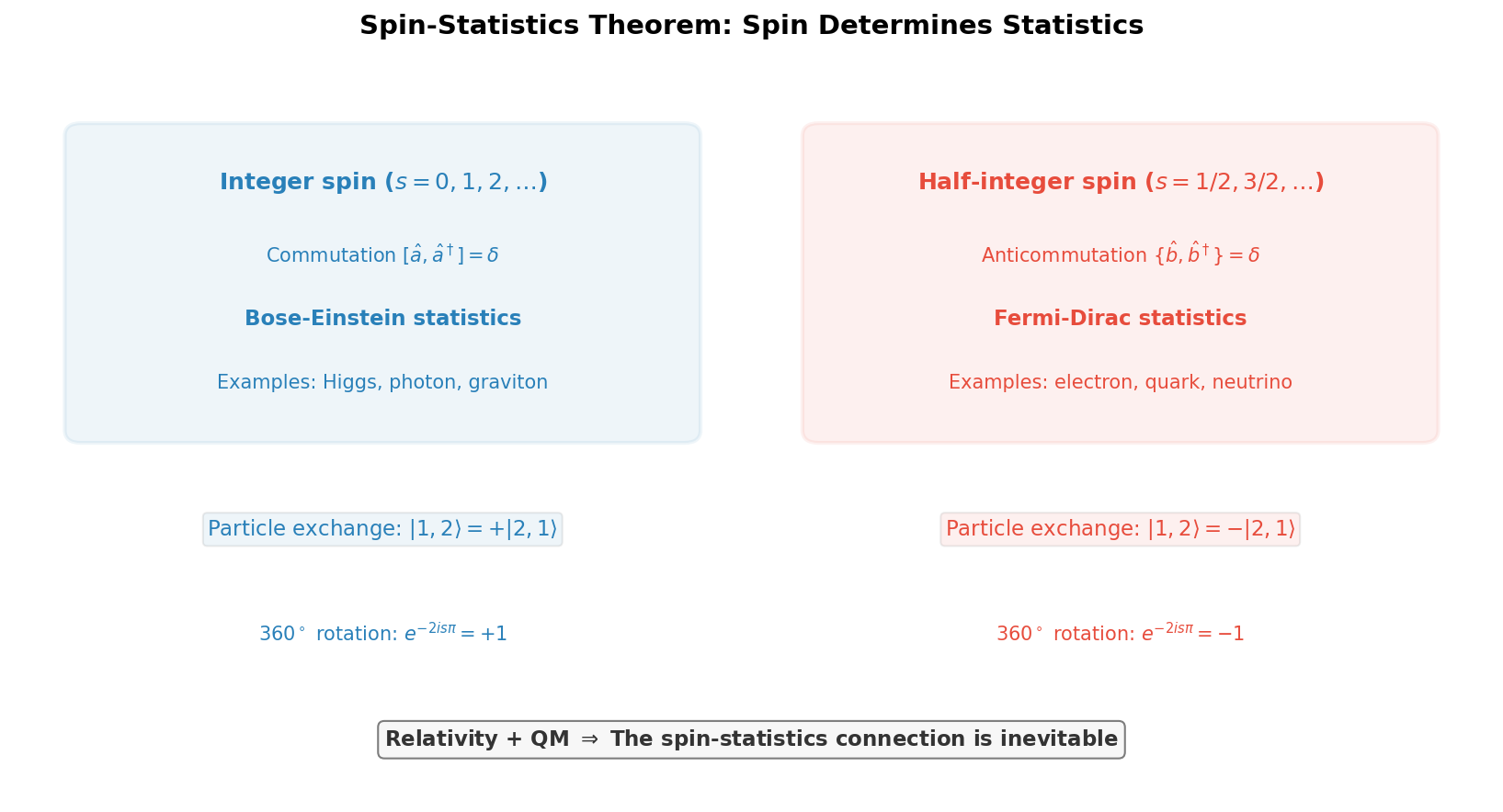
Fig. 5.6: Conceptual diagram of the spin-statistics theorem. Integer-spin fields become bosons with commutation relations, and half-integer-spin fields become fermions with anticommutation relations. This connection is unavoidably derived from relativistic quantum field theory.
✅ Comprehension Check: State why the spin-statistics theorem cannot be proven within non-relativistic quantum mechanics.
Answer
Non-relativistic quantum mechanics does not require Lorentz invariance, so causality (vanishing of commutators in the spacelike region) and boost transformation properties (the distinction between left-handed and right-handed) don't enter the discussion. The connection between spin and statistics can only be derived by combining relativity (Lorentz invariance) with quantum mechanics.
5.9 \(C, P, T\) Transformations
🟡 Lina: Finally, let's look at 3 discrete symmetries for the Dirac field. These are the quantum field theory formulations of what we conceptually learned in Quantum Mechanics Ch. 26.
Table 5.4: Summary of \(C\), \(P\), \(T\) transformations
| Transformation | Operation | Action on Dirac field | Characteristic |
|---|---|---|---|
| \(P\) (parity) | \(\boldsymbol{x} \to -\boldsymbol{x}\) | \(\psi_L \leftrightarrow \psi_R\) (mediated by \(\gamma^0\)) | Unitary |
| \(C\) (charge conjugation) | Particle \(\leftrightarrow\) antiparticle | \(\hat{b} \leftrightarrow \hat{c}\) | Unitary |
| \(T\) (time reversal) | \(t \to -t\) | Mixes spinor components via \(\gamma^1\gamma^3\) | Anti-unitary |
Parity \(P\) — Space Inversion
🟡 Lina: The parity transformation \(P\) is the operation of inverting spatial coordinates: \(\boldsymbol{x} \to -\boldsymbol{x}\). For the Dirac field:
🔵 Kai: A factor of \(\gamma^0\) appears. Why?
🟡 Lina: The upper 2 components (left-handed) and lower 2 components (right-handed) of the Dirac spinor are exchanged under parity. There are several representations (concrete choices of matrices) for the \(\gamma\) matrices, but in the chiral representation where the left-/right-handed structure is most transparent:
This matrix swaps the upper and lower 2 components—i.e., it exchanges \(\psi_L\) and \(\psi_R\). Since parity is a "spatial reflection," the intuition that left-handed and right-handed are exchanged makes sense, right?
⚪ Mei: It's the same sense as a mirror swapping right and left hands.
🟡 Lina: Right. For creation and annihilation operators:
The sign of the momentum is reversed, and antiparticles additionally acquire a minus sign. Let me introduce a new concept here. Intrinsic parity is the inherent phase factor that a state acquires under parity transformation. Why is such a thing needed? Because parity "flips space," but depending on the particle's internal structure (the relationship between upper and lower spinor components), an additional phase may or may not appear upon flipping. This is an inherent property determined for each particle type, a quantum number independent of momentum and spin—"inherent" in the same sense that charge is determined by particle type.
🔵 Kai: Looking at equation (5.29), \(\hat{b}\) has no extra sign but \(\hat{c}\) has a minus—is this the difference in intrinsic parity?
🟡 Lina: Exactly. Looking at equation (5.29), the transformation of \(\hat{b}\) has no extra sign (\(P^{-1}\hat{b}^s_{\boldsymbol{p}}P = \hat{b}^s_{-\boldsymbol{p}}\)), while the transformation of \(\hat{c}\) has a minus (\(P^{-1}\hat{c}^s_{\boldsymbol{p}}P = -\hat{c}^s_{-\boldsymbol{p}}\)). This extra minus is the quantum number called "intrinsic parity"—if we conventionally define the particle's intrinsic parity as \(+1\) (this convention is just that—a convention; physical consequences are determined by the product of particle and antiparticle intrinsic parities), then the antiparticle's intrinsic parity is \(-1\). That is, for fermions the product of particle and antiparticle intrinsic parities is \(-1\) (\(\eta_P(\text{particle}) \times \eta_P(\text{antiparticle}) = -1\)). This is a consequence determined by the structure of the Dirac equation, and has been experimentally confirmed (e.g., from the angular distribution of \(\pi^0 \to e^+e^-\)).
Charge Conjugation \(C\) — Exchanging Particles and Antiparticles
🟡 Lina: Charge conjugation \(C\) is the operation of exchanging particles and antiparticles.
⚪ Mei: So applying \(C\) to the charge operator \(\hat{Q} = \hat{N}_b - \hat{N}_c\) from equation (5.26) swaps particle and antiparticle numbers, giving \(C^{-1}\hat{Q}\,C = -\hat{Q}\).
🟡 Lina: Exactly. And only particles that are identical to their own antiparticles can be eigenstates of \(C\). The photon has \(C\)-parity \(-1\), and the neutral pion \(\pi^0\) has \(C\)-parity \(+1\).
✅ Comprehension Check: What kind of particles can be eigenstates of charge conjugation \(C\)? State the reason.
Answer
Only particles that are identical to their own antiparticles (e.g., photon, \(\pi^0\)) can be eigenstates of \(C\). Since \(C\) exchanges particles and antiparticles, when the particle and antiparticle are different, \(C\) maps to a different state, and the state cannot be an eigenstate.
Time Reversal \(T\) — Reversing the Flow of Time
🟡 Lina: Time reversal \(T\) is the operation \(t \to -t\). However, \(T\) has a decisively different property from the other two.
🔵 Kai: What's different?
🟡 Lina: \(T\) is an anti-unitary operator. That means \(T(c|\psi\rangle) = c^* T|\psi\rangle\) (it complex conjugates numbers). Recall what we learned in Quantum Mechanics Ch. 26.
The explicit form of the matrix \(\gamma^1\gamma^3\) depends on the representation of the \(\gamma\) matrices, but its role is to "mix spinor components so that the Dirac equation remains invariant under \(t \to -t\)." Why this particular combination? It's the matrix determined from the Clifford algebra that is needed to compensate for the sign change of \(\gamma^0\partial_0\) under \(t \to -t\). Derivation details are in Appendix B. The anti-unitarity of \(T\) comes from the fact that under \(t \to -t\) in the Schrödinger equation \(i\partial_t|\psi\rangle = H|\psi\rangle\), the sign of \(i\) must also be flipped for the equation to remain invariant.
⚪ Mei: So only \(T\) is anti-unitary, while \(C\) and \(P\) are unitary—time reversal alone is special.
CPT Theorem
🟡 Lina: In nature, \(C\), \(P\), \(T\) can each individually be violated. The weak interaction violates \(P\), and also violates \(CP\). But—
CPT theorem: In a Lorentz-invariant, local quantum field theory, the combined transformation \(CPT\) of all three is always a symmetry.
🔵 Kai: Combining all three is always a symmetry!?
🟡 Lina: Yes. As a consequence of the CPT theorem, particles and antiparticles must have the same mass and lifetime. This has been experimentally verified to extremely high precision. If CPT were violated, it would mean either Lorentz invariance or locality is broken—that would be a seismic event shaking the foundations of physics. The relationships among \(C\), \(P\), \(T\) are summarized in Fig. 5.7 "C, P, T discrete symmetries and CPT theorem".
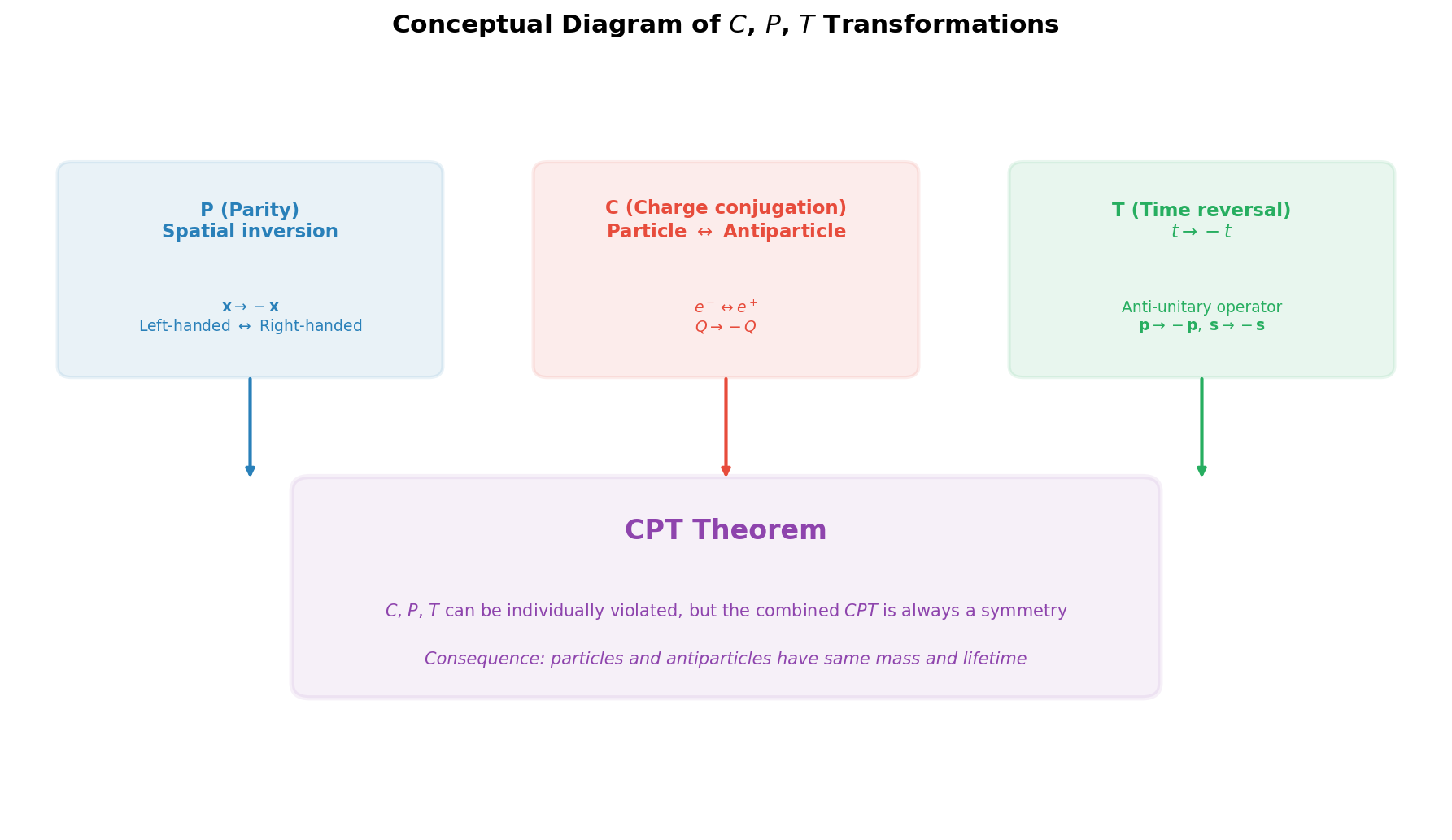
Fig. 5.7: C, P, T discrete symmetries and CPT theorem. The 3 discrete symmetries \(C\) (charge conjugation), \(P\) (parity), \(T\) (time reversal). Each can individually be violated, but the CPT theorem guarantees that the simultaneous transformation of all three is always a symmetry.
✅ Comprehension Check: State 2 specific relationships between particles and antiparticles that follow from the CPT theorem.
Answer
(1) Particles and antiparticles have the same mass. (2) Particles and antiparticles have the same lifetime. (Also correct: "same spin," "same magnitude but opposite sign of magnetic moment," etc.)
📝 Exercises:
- Composition of \(C, P, T\) transformations and the CPT theorem → Problem A-2. \(C\), \(P\), \(T\) Transformations and the \(CPT\) Theorem
5.10 Summary of This Chapter
🟡 Lina: Let's review today's content.
⚪ Mei: Let me organize.
-
The Dirac equation is written as \((i\not\!\partial - m)\psi = 0\) using \(4 \times 4\) \(\gamma\) matrices satisfying the Clifford algebra \(\{\gamma^\mu, \gamma^\nu\} = 2\eta^{\mu\nu}\). The wave function \(\psi\) is a 4-component Dirac spinor.
-
The Lorentz algebra decomposes into \(\mathfrak{su}(2) \oplus \mathfrak{su}(2)\), and the Dirac spinor corresponds to the \((1/2, 0) \oplus (0, 1/2)\) representation. It combines left-handed and right-handed Weyl spinors.
-
The Dirac field Lagrangian is \(\mathcal{L} = \bar{\psi}(i\not\!\partial - m)\psi\), and the conjugate momentum is \(\Pi = i\psi^\dagger\).
-
Quantizing with commutation relations leads to breakdown—the \([\hat{c}, \hat{c}^\dagger]\) for antiparticles picks up a minus sign, making the Hamiltonian energy unbounded below.
-
Quantizing with anticommutation relations \(\{\hat{b}, \hat{b}^\dagger\} = \delta\), \(\{\hat{c}, \hat{c}^\dagger\} = \delta\) makes the Hamiltonian positive-definite: \(:\hat{H}: = \sum E_{\boldsymbol{p}}(\hat{b}^\dagger\hat{b} + \hat{c}^\dagger\hat{c})\), and a stable vacuum exists.
-
From anticommutation relations, the Pauli exclusion principle \((\hat{b}^\dagger)^2 = 0\) and Fermi-Dirac statistics automatically follow.
-
Spin-statistics theorem: integer spin → bosons (commutation relations), half-integer spin → fermions (anticommutation relations). This is one of the deepest consequences of relativistic quantum field theory.
-
\(C, P, T\) transformations: respectively particle↔antiparticle, space inversion, time reversal. Each can individually be violated, but CPT is always a symmetry.
🔵 Kai: For the scalar field quantization, "imposing commutation relations makes the energy positive-definite," whereas for the Dirac field, "commutation relations break things so anticommutation relations are necessary." Having actually experienced the breakdown with commutation relations, I can truly feel that anticommutation relations are chosen not "reluctantly" but "inevitably." Just going from spin 0 to spin 1/2, so many new issues arise. I wonder about spin-1 photons—integer spin should mean commutation relations are fine, but might some different problem arise?
🟡 Lina: Good question. Photons have integer spin, so quantizing with commutation relations is correct. But photons harbor a different troublesome issue called "gauge freedom," and naively attempting canonical quantization hits a wall. That's the topic for the next chapter.
And today's drama centered on "spin." Whether spin is integer or half-integer determines the quantization prescription, determines the statistics, and determines the stability of matter. Without quantum field theory, this deep connection would never have been visible.
Preview of the Next Chapter
Having completed the quantization of spin 0 (scalar field) and spin 1/2 (Dirac field), what remains is spin 1—the photon field. However, the electromagnetic field harbors a troublesome redundancy called "gauge freedom," and naively attempting canonical quantization hits a new wall where the conjugate momentum vanishes. In Ch. 6, we'll overcome this wall using gauge-fixing techniques and learn how to correctly quantize only the physical polarization degrees of freedom of the photon. Once the quantization of all three free fields—scalar field (Ch. 4), Dirac field (this chapter), and electromagnetic field (Ch. 6)—is complete, we'll be fully prepared to introduce interactions in Ch. 7.
Exercises
📝 Exercises:
- Deriving properties of \(\gamma\) matrices from the Clifford algebra → Problem B-1. Basic Calculations with the Clifford Algebra
- Comparison of Dirac field Hamiltonian with commutation vs. anticommutation relations → Problem M-1. Failure of Quantization via Commutation Relations
- Derivation of the Pauli exclusion principle from anticommutation relations → Problem M-2. Derivation of the Pauli Exclusion Principle
- Composition of \(C, P, T\) transformations and the CPT theorem → Problem A-2. \(C\), \(P\), \(T\) Transformations and the \(CPT\) Theorem
- Scalar field anticommutation relations and violation of causality → Problem B-9. Anticommutation Relations for a Scalar Field and Violation of Causality
References
- Quantum Field Theory for the Gifted Amateur (Lancaster & Blundell) Chapter 36 "The Dirac Equation," Chapter 37 "Transformation Properties of Spinors," Chapter 38 "Quantizing the Dirac Field"
- Quantum Field Theory (David Tong, Cambridge) Chapter 4 "The Dirac Equation," Chapter 5 "Quantizing the Dirac Field"
- 場の量子論 — 不変性と自由場を中心にして (Sakamoto Masato) Chapter 4 "Derivation of the Dirac Equation and γ Matrices," Chapter 5 "Lorentz Transformation Properties of the Dirac Equation," Chapter 12 "Quantization of the Dirac Field"
- Quantum Field Theory and the Standard Model (Schwartz) Chapter 8 "Spinors and the Dirac Equation," Chapter 9 "The Spin-Statistics Theorem"
Feedback on this page
Let us know if something was unclear, incorrect, or could be improved.