Appendix C: Fourier Analysis and the δ Function
Story so far:
In Appendix B, we organized the foundations of linear algebra and Hilbert spaces, seeing how concepts such as vectors, inner products, bases, and complete sets can be extended from finite dimensions to infinite dimensions. In this chapter, we organize "Fourier analysis" and the "δ function," which play central roles in that infinite-dimensional extension, focusing on the scope needed for physics.
Goals of this chapter
- Understand the Fourier series, which represents arbitrary functions as superpositions of trigonometric functions (complex exponentials), and derive the Fourier transform obtained by taking the period to infinity
- Through this, acquire the mathematical foundation that bridges position representation and momentum representation in quantum mechanics
- Furthermore, derive the powerful properties of Fourier transforms—Parseval's equality and the convolution theorem—and organize the definition, properties, and relationship to complete sets of the Dirac δ function
- These become essential tools for working with wave functions from Ch. 7 onward
C.1 Fourier Series — Orthogonality of Trigonometric Functions and Determining Coefficients
🟡 Lina: In Appendix B, you learned about "basis expansions." Finite-dimensional vectors could be expanded in orthonormal bases. Today we extend that idea to functions.
🔵 Kai: What does it mean to "expand" a function?
🟡 Lina: For example, representing a function \(f(x)\) that repeats with period \(L\) (meaning it satisfies \(f(x + L) = f(x)\)) as a "sum" of simpler functions. Specifically, we use \(\sin\) and \(\cos\). This is the Fourier series. It's sufficient to consider one period, say the interval \([0, L]\).
🔵 Kai: Even for arbitrarily complicated functions?
🟡 Lina: For virtually all "well-behaved" functions that appear in physics, yes. Historically, Fourier made this claim in 1807 for "heat conduction problems" and astonished the mathematicians of his day.
Orthogonality of Trigonometric Functions
🟡 Lina: First, the key is the orthogonality of trigonometric functions. In Appendix B, you called vectors "orthogonal" when their inner product is zero, right? The same idea works for functions. We define the "inner product" of functions \(f(x)\) and \(g(x)\) as follows:
Here \(f(x)^*\) is the complex conjugate. As you learned in Appendix B, for complex vector inner products we write \(\langle \mathbf{a}, \mathbf{b}\rangle = \sum_i a_i^* b_i\), putting the complex conjugate on one side. This is necessary so that "the inner product with itself \(\langle f, f\rangle\) is always a positive real number (the square of the norm)." For real functions, \(f^* = f\), so it simply becomes the integral of \(f(x) \cdot g(x)\).
⚪ Mei: The "sum" in the vector inner product \(\mathbf{a} \cdot \mathbf{b} = \sum_i a_i b_i\) gets replaced by an "integral." A natural extension from discrete to continuous.
🟡 Lina: Exactly. Using this inner product, the following orthogonality relations hold for trigonometric functions. With \(m, n\) as positive integers (\(m, n = 1, 2, 3, \ldots\)):
Here \(\delta_{mn}\) is the Kronecker delta — a symbol that equals \(1\) when \(m = n\) and \(0\) when \(m \neq n\).
🔵 Kai: Why does the integral become zero when \(m \neq n\)?
🟡 Lina: You can show it using product-to-sum formulas. From the addition formulas \(\cos(A + B) = \cos A\cos B - \sin A\sin B\) and \(\cos(A - B) = \cos A\cos B + \sin A\sin B\), adding both sides gives \(\cos(A+B) + \cos(A-B) = 2\cos A\cos B\), so dividing by 2: \(\cos A\cos B = \frac{1}{2}[\cos(A+B) + \cos(A-B)]\). For example, in the case of equation (C.2), setting \(A = \frac{2\pi m}{L}x\) and \(B = \frac{2\pi n}{L}x\):
When \(m \neq n\), both \((m+n)\) and \((m-n)\) are nonzero integers, so integrating \(\cos\) over an integer number of periods gives zero. To verify explicitly, for any nonzero integer \(p\): \(\int_0^L \cos\!\left(\frac{2\pi p}{L}x\right)dx = \left[\frac{L}{2\pi p}\sin\!\left(\frac{2\pi p}{L}x\right)\right]_0^L = \frac{L}{2\pi p}[\sin(2\pi p) - \sin(0)] = 0\) (since \(\sin\) is zero at integer multiples of \(2\pi\)). Intuitively, the positive peaks and negative troughs of \(\cos\) are symmetric, and the area over an integer number of periods cancels out.
🔵 Kai: Ah, I see. Integrating \(\cos\) over one full period, the peaks and troughs cancel to give zero, and the same holds for any integer number of periods. But what about when \(m = n\)? If you multiply the same function by itself you get \(\cos^2\), which is always positive, so it shouldn't cancel out, right?
🟡 Lina: Good intuition. When \(m = n\), \(\cos\!\left(\frac{2\pi(m-n)}{L}x\right) = \cos(0) = 1\) (a constant), so the integrand becomes:
The first term \(\cos\!\left(\frac{4\pi n}{L}x\right)\) has period \(L/(2n)\), so its integral over \([0, L]\) covers \(2n\) full periods—and integrating \(\cos\) over an integer number of periods gives zero. The integral of the constant \(1\) is \(L\). Therefore the total is \(\frac{1}{2}[0 + L] = L/2\).
⚪ Mei: So cosines with different frequencies are "orthogonal," and the inner product is nonzero only when the frequencies match. Exactly the same structure as orthonormal basis vectors.
Determining the Fourier Coefficients
🟡 Lina: Using this orthogonality, we can expand a function \(f(x)\) as follows. This is the Fourier series:
By the way, the constant function \(1\) is also orthogonal to \(\cos\) and \(\sin\). For \(n \geq 1\), \(\int_0^L 1 \cdot \cos\!\left(\frac{2\pi n}{L}x\right)dx = 0\) and \(\int_0^L 1 \cdot \sin\!\left(\frac{2\pi n}{L}x\right)dx = 0\)—this follows from the fact that integrating \(\cos\) or \(\sin\) over one full period gives zero. So \(a_0/2\) (the constant term) can also be extracted independently from the other terms.
🟡 Lina: Look at Fig. C.1 "Reconstruction of a square wave by Fourier series and the Gibbs phenomenon". It shows a square wave with period \(2\pi\)—a function that equals \(+1\) for \(0 < x < \pi\) and \(-1\) for \(-\pi < x < 0\)—being approximated by a Fourier series. Looking at just one period, it has the same shape as the sign function \(\mathrm{sgn}(x)\), which returns \(+1\) for \(x > 0\) and \(-1\) for \(x < 0\). As the number of terms \(N\) increases, it approaches the square wave more closely, but a slight overshoot remains near the discontinuities. This is called the Gibbs phenomenon, and it's known that even as \(N \to \infty\), an overshoot of about 9% persists.
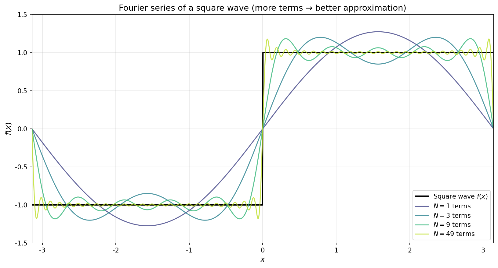
Fig. C.1: Reconstruction of a square wave by Fourier series and the Gibbs phenomenon. The square wave \(f(x) = \mathrm{sgn}(x)\) approximated by a Fourier series. As the order \(N\) increases, the approximation approaches the square wave. At discontinuities, a slight overshoot known as the "Gibbs phenomenon" remains (a limitation of partial sums of the series).
🔵 Kai: Even summing infinitely many terms doesn't give perfect agreement?
🟡 Lina: It does agree everywhere except at the discontinuities. At the discontinuity itself, the Fourier series converges to the average of the left and right values. Since functions in physics are usually smooth, this rarely causes practical problems.
The coefficients can be "extracted" using orthogonality:
🔵 Kai: Why does multiplying by \(\cos\) and integrating give us \(a_n\)?
🟡 Lina: Remember the vector case. To extract the component along basis vector \(\mathbf{e}_n\), you computed the inner product \(\mathbf{e}_n \cdot \mathbf{v}\), right? It's the same thing. If you multiply both sides of equation (C.5) by \(\cos\!\left(\frac{2\pi m}{L}x\right)\) and integrate from \(0\) to \(L\), thanks to the orthogonality relations (C.2) and (C.4), only the \(\cos\) term with \(n = m\) survives—the contribution from the constant term \(a_0/2\) is \(\frac{a_0}{2}\int_0^L \cos\!\left(\frac{2\pi m}{L}x\right)dx = 0\) (integrating \(\cos\) over an integer number of periods gives zero for \(m \geq 1\)), the \(\sin\) terms vanish by (C.4), and the \(\cos\) terms with \(n \neq m\) vanish by (C.2). We end up with:
Solving for \(a_m\) gives equation (C.6).
⚪ Mei: The notation \(a_0/2\) makes sense because substituting \(n = 0\) into the \(a_n\) formula gives \(\cos(0) = 1\), so \(a_0 = \frac{2}{L}\int_0^L f(x)\,dx\), which is twice the average value of the function. So \(a_0/2\) is the average value itself.
🟡 Lina: Perfect summary.
✅ Comprehension Check: What quantity of the original function \(f(x)\) does the Fourier series coefficient \(a_0/2\) correspond to?
Answer
\(a_0/2\) corresponds to the average value of the function \(f(x)\) over one period. Since \(a_0 = \frac{2}{L}\int_0^L f(x)\,dx\), we have \(a_0/2 = \frac{1}{L}\int_0^L f(x)\,dx\), which is the average value of \(f(x)\) over the interval \([0, L]\).
✅ Comprehension Check: To find \(b_n\) from equation (C.5), what should you multiply both sides by before integrating?
Answer
Multiply by \(\sin\!\left(\frac{2\pi m}{L}x\right)\) and integrate from \(0\) to \(L\). By orthogonality (C.3) and (C.4), only the \(\sin\) term with \(n = m\) survives, giving \(b_m \cdot L/2\).
📝 Exercises:
- Find the Fourier coefficients \(a_n, b_n\) for \(f(x) = x\) on the interval \([0, L]\) → Problem M-1. Find the Fourier coefficients and of the function defined on the interval , and write down the Fourier series (Equation (C.5
C.2 Complex Fourier Series — A Unified Expression via Euler's Formula
🟡 Lina: Equation (C.5) mixes two types, \(\sin\) and \(\cos\), which is somewhat unwieldy. Using Euler's formula, which you learned in Appendix A, we can rewrite it in a much cleaner form.
From this:
(These are formulas derived in Appendix A. Adding \(e^{i\theta}\) and \(e^{-i\theta}\) cancels the \(\sin\) leaving \(\cos\), and subtracting cancels the \(\cos\) leaving \(\sin\)—that's all there is to it.)
🔵 Kai: So \(\sin\) and \(\cos\) can be unified into a single exponential function.
🟡 Lina: Right. Let's write the wavenumber as \(k_n \equiv \frac{2\pi n}{L}\). Ultimately we'll use \(n\) as any integer (positive, negative, or zero). Why negative \(n\) becomes necessary will become clear naturally as we rewrite equation (C.5). First, for each term with \(n > 0\), let's replace \(\cos\) and \(\sin\) using equation (C.9):
Writing out the intermediate steps carefully: from \(\cos(k_n x) = \frac{e^{ik_n x} + e^{-ik_n x}}{2}\), the coefficient of \(e^{ik_n x}\) is \(\frac{a_n}{2}\), and the coefficient of \(e^{-ik_n x}\) is also \(\frac{a_n}{2}\). From \(\sin(k_n x) = \frac{e^{ik_n x} - e^{-ik_n x}}{2i}\), the coefficient of \(e^{ik_n x}\) is \(\frac{b_n}{2i}\), and the coefficient of \(e^{-ik_n x}\) is \(-\frac{b_n}{2i}\). Combined, the coefficient of \(e^{ik_n x}\) is \(\frac{a_n}{2} + \frac{b_n}{2i}\), and the coefficient of \(e^{-ik_n x}\) is \(\frac{a_n}{2} - \frac{b_n}{2i}\). To compute \(\frac{1}{i}\), we want to rationalize the denominator, so multiply numerator and denominator by \(i\): \(\frac{1}{i} = \frac{i}{i^2} = \frac{i}{-1} = -i\). Therefore \(\frac{b_n}{2i} = \frac{b_n}{2}\cdot(-i) = -\frac{ib_n}{2}\). Substituting this:
🔵 Kai: I see, so they've been grouped into \(e^{ik_n x}\) and \(e^{-ik_n x}\).
🟡 Lina: Looking at this expression, the coefficient of \(e^{ik_n x}\) is \(\frac{a_n - ib_n}{2}\) and the coefficient of \(e^{-ik_n x}\) is \(\frac{a_n + ib_n}{2}\). So we define:
- \(c_n \equiv \dfrac{a_n - ib_n}{2}\) (for \(n > 0\))
- \(c_{-n} \equiv \dfrac{a_n + ib_n}{2}\) (for \(n > 0\))
- \(c_0 \equiv \dfrac{a_0}{2}\)
Let's verify—substituting into \(c_n\,e^{ik_n x} + c_{-n}\,e^{-ik_n x}\) gives \(\frac{a_n - ib_n}{2}e^{ik_n x} + \frac{a_n + ib_n}{2}e^{-ik_n x}\). This is exactly the right-hand side we computed above, so it matches the original form \(a_n\cos(k_n x) + b_n\sin(k_n x)\). The \(n = 0\) term is \(c_0\,e^{i \cdot 0 \cdot x} = c_0 = a_0/2\), giving the constant term.
Let me explain "why we named it \(c_{-n}\)." In the definition \(k_n = \frac{2\pi n}{L}\), if we substitute a negative integer for \(n\), we get \(k_{-n} = \frac{2\pi(-n)}{L} = -\frac{2\pi n}{L} = -k_n\). That is, \(e^{-ik_n x} = e^{ik_{-n} x}\)—\(-k_n\) and \(k_{-n}\) are the same thing. So \(c_{-n}\,e^{-ik_n x}\) can be rewritten as \(c_{-n}\,e^{ik_{-n} x}\). This is the "term with index \(-n\)" itself.
⚪ Mei: So by reinterpreting the \(e^{-ik_n x}\) terms as "negative index terms," we can combine positive and negative \(n\) into a single sum.
🟡 Lina: Exactly. Equation (C.5) can be written as "the \(n = 0\) term" + "a sum over \(n > 0\) terms," but thanks to naming the coefficient of \(e^{-ik_n x}\) as \(c_{-n}\), we can reinterpret "terms with negative \(n\)" and combine everything into a single sum from \(n = -\infty\) to \(+\infty\):
Here the complex Fourier coefficients \(c_n\) are:
(Since the function is periodic, the integration range gives the same value whether we use \([0, L]\) or \([-L/2, L/2]\) or any other single period. In Section C.3, we'll use \([-L/2, L/2]\) to make it easier to take the \(L \to \infty\) limit.)
⚪ Mei: The range of summation expanded from \(n = -\infty\) to \(+\infty\) because decomposing \(\cos\) and \(\sin\) into \(e^{+ik_n x}\) and \(e^{-ik_n x}\) made negative \(n\) necessary. 🟡 Lina: Right. And let's verify the derivation of equation (C.11). We'll look at the orthogonality of complex exponentials. Using the inner product definition (C.1) with \(f = e^{ik_n x}\) and \(g = e^{ik_m x}\): \(\langle e^{ik_n x}, e^{ik_m x}\rangle = \int_0^L (e^{ik_n x})^* e^{ik_m x}\,dx = \int_0^L e^{-ik_n x} e^{ik_m x}\,dx\) (the complex conjugate of \(e^{ik_n x}\) is \(e^{-ik_n x}\)). Combining the exponents:
When \(m \neq n\), the integral is \(\left[\frac{L}{i \cdot 2\pi(m-n)}e^{i \frac{2\pi(m-n)}{L} x}\right]_0^L = \frac{L}{i \cdot 2\pi(m-n)}\left[e^{i 2\pi(m-n)} - e^{0}\right]\), but since \((m-n)\) is an integer, \(e^{i2\pi(m-n)} = \cos(2\pi(m-n)) + i\sin(2\pi(m-n)) = 1\) (since \(\cos\) and \(\sin\) return to their original values at integer multiples of \(2\pi\)), and \(e^0 = 1\), so \([1 - 1] = 0\). When \(m = n\), the integrand is \(e^0 = 1\), so the integral is \(L\).
🔵 Kai: The same logic as with trigonometric functions. Using orthogonality to "extract" coefficients.
🟡 Lina: Multiply both sides of equation (C.10) by \(e^{-ik_m x}\) and integrate from \(0\) to \(L\). We choose \(e^{-ik_m x}\) because we want to use orthogonality (C.12)—multiplying \(e^{ik_n x}\) by \(e^{-ik_m x}\) gives \(e^{i(k_n - k_m)x}\), and only when \(n = m\) does the integral equal \(L\). In other words, \(e^{-ik_m x}\) acts as a "filter" that selects only the \(n = m\) term:
Therefore \(c_m = \frac{1}{L}\int_0^L f(x)\,e^{-ik_m x}\,dx\). This is exactly equation (C.11).
✅ Comprehension Check: For a real function \(f(x)\), what relationship exists between \(c_n\) and \(c_{-n}\)?
Answer
If \(f(x)\) is real, then \(f(x)^* = f(x)\), so \(c_n^* = \frac{1}{L}\int_0^L f(x)\,e^{+ik_n x}\,dx = c_{-n}\). That is, \(c_{-n} = c_n^*\) (complex conjugate relationship).
C.3 Fourier Transform — The Limit of Taking the Period to Infinity
🟡 Lina: The Fourier series was a tool for handling "functions that repeat with period \(L\)." But in quantum mechanics, we want to handle wave functions that extend over all of space \((-\infty, +\infty)\). To remove the periodicity constraint, we take the limit \(L \to \infty\).
🔵 Kai: Make the period infinite? What changes?
🟡 Lina: The wavenumber \(k_n = \frac{2\pi n}{L}\) takes values at each integer \(n\), so the spacing between adjacent wavenumbers is \(\Delta k = k_{n+1} - k_n = \frac{2\pi(n+1)}{L} - \frac{2\pi n}{L} = \frac{2\pi}{L}\). As \(L \to \infty\), \(\Delta k \to 0\), and the discrete sum \(\sum_n\) transitions to a continuous integral \(\int dk\). Let's see this concretely.
Derivation
🟡 Lina: Let me rewrite equation (C.10):
We substitute \(c_n\) from equation (C.11). The integration range in (C.11) was \([0, L]\), but to make it easier to take the \(L \to \infty\) limit, I'll change it to \([-L/2, L/2]\) (since the function is periodic, integrating over any single period gives the same result—I'll explain shortly):
🔵 Kai: Wait, the integration range changed from \([0, L]\) to \([-L/2, L/2]\)—is that okay?
🟡 Lina: Good question. A function with period \(L\) satisfies \(f(x + L) = f(x)\), so the integral value is the same no matter where you start one period. Intuitively, no matter where you cut a periodically repeating pattern, if you take exactly one period's worth, you get the same content. Think of wallpaper—no matter where you cut, if you cut out one pattern length, you get the same design. The integral value works the same way. To verify with a concrete example, \(1 + \cos x\) has period \(2\pi\), and \(\int_0^{2\pi}(1+\cos x)\,dx = 2\pi\) and \(\int_{-\pi}^{\pi}(1+\cos x)\,dx = 2\pi\)—both give the same value because each contains exactly one peak. By the same reasoning, \([0, L]\) and \([-L/2, L/2]\) are equivalent. When taking the \(L \to \infty\) limit, \([-L/2, L/2]\) is easier to work with since it's symmetric about the origin. You might wonder, "Doesn't the function stop being periodic when \(L \to \infty\)?" And you'd be right. The final equations (C.14) and (C.15) apply to general functions without assuming periodicity. The period \(L\) is merely a "scaffold" used during the derivation, which we remove in the \(L \to \infty\) limit.
⚪ Mei: By removing the "scaffold" of period \(L\) in the \(L \to \infty\) limit, we can handle general functions without periodicity.
🟡 Lina: Next, to make the \(L \to \infty\) limit easy to take, I'll rewrite \(\frac{1}{L}\) in terms of the wavenumber spacing \(\Delta k = \frac{2\pi}{L}\). Since \(\frac{1}{L} = \frac{\Delta k}{2\pi}\):
⚪ Mei: Since \(\Delta k \to 0\) as \(L \to \infty\), the sum \(\sum_n \Delta k\) becomes \(\int dk\).
🟡 Lina: Right. Remember the Riemann sum approximation you learned in high school—dividing an interval into narrow strips with area \(f(k_n)\,\Delta k\) and summing them, in the limit of infinitely fine division, gives the definite integral \(\int f(k)\,dk\). Exactly the same thing is happening here. \(\Delta k = 2\pi/L\) is the "strip width," and as \(L \to \infty\) the width approaches zero, transitioning from a discrete sum to a continuous integral. In the \(L \to \infty\) limit:
Here we name the expression in brackets \(\tilde{f}(k)\). This is the Fourier transform:
And the formula that recovers the original function is the inverse Fourier transform:
🔵 Kai: Oh, they have a symmetric form. Though it bugs me a little that the \(2\pi\) factor appears on only one side.
🟡 Lina: Good point. There are actually 3 conventions for distributing the \(2\pi\), used in different areas of physics:
Table C.1: Conventions for distributing 2π in Fourier transforms
| Convention | Transform | Inverse transform | Main field of use |
|---|---|---|---|
| (a) | \(\tilde{f}(k) = \int f(x)\,e^{-ikx}\,dx\) | \(f(x) = \frac{1}{2\pi}\int \tilde{f}(k)\,e^{ikx}\,dk\) | Field theory, systems with \(\hbar = 1\) |
| (b) | \(\tilde{f}(k) = \frac{1}{\sqrt{2\pi}}\int f(x)\,e^{-ikx}\,dx\) | \(f(x) = \frac{1}{\sqrt{2\pi}}\int \tilde{f}(k)\,e^{ikx}\,dk\) | Quantum mechanics (symmetric convention) |
| (c) | \(\tilde{f}(\nu) = \int f(t)\,e^{-2\pi i \nu t}\,dt\) | \(f(t) = \int \tilde{f}(\nu)\,e^{2\pi i \nu t}\,d\nu\) | Engineering, signal processing |
In Quantum Mechanics we primarily use convention (b). It's the form most commonly seen in quantum mechanics textbooks, and it's easy to remember because the transform and inverse transform have a completely symmetric form. The Parseval equality we'll show later also takes its cleanest form. Equations (C.14) and (C.15) emerged naturally from the \(L \to \infty\) limit (convention (a)), but from now on I'll unify everything under convention (b). The difference is simple: convention (b)'s \(\tilde{f}(k)\) is convention (a)'s \(\tilde{f}(k)\) multiplied by \(1/\sqrt{2\pi}\). In other words, we use the same symbol \(\tilde{f}\), but the definitions differ by a factor of \(1/\sqrt{2\pi}\). From here on in this chapter, whenever I write \(\tilde{f}(k)\), I always mean the convention (b) definition:
⚪ Mei: The transform and inverse transform take the same form. Only the sign of the exponent differs. Symmetric and easy to remember.
Physical Meaning
🟡 Lina: Physically speaking, \(f(x)\) is a function in "position space" and \(\tilde{f}(k)\) is a function in "wavenumber space." In quantum mechanics, since \(p = \hbar k\) (the de Broglie relation—you learned this in Ch. 2), \(\tilde{f}(k)\) is directly connected to the representation in "momentum space." We'll cover this in detail in Ch. 10, but the Fourier transform is precisely the tool that bridges "a wave function written using position \(x\)" and "a wave function written using momentum \(p\) (i.e., wavenumber \(k\))"—and in fact, \(|\tilde{f}(k)|^2\) gives the "probability density for having momentum \(\hbar k\)."
🔵 Kai: Wait a moment. What does it mean that \(|\tilde{f}(k)|^2\) becomes the "probability density for momentum"? I don't understand why the absolute value squared of a wavenumber-space function becomes a probability...
🟡 Lina: Good question. At this stage, I'll just preview that "this is how it gets interpreted." We'll prove it rigorously in Ch. 10, combined with the probabilistic interpretation of the wave function. For now, just hold onto this intuition: "The Fourier transform tells us how much of each wavenumber component is contained"—and since by the de Broglie relation \(p = \hbar k\), the component at wavenumber \(k\) corresponds to momentum \(\hbar k\), we can read off "what momenta this particle has, and in what proportions." Why the "proportion" takes the form \(|\tilde{f}(k)|^2\)—that is, why the absolute value squared gives the probability density—can only be properly understood in Ch. 10 when combined with Born's probability interpretation.
🔵 Kai: I see, so "we can determine the proportions" is something I can understand with the current mathematics, but "this becomes a probability density" requires a physical interpretation.
✅ Comprehension Check: What is the physical reason that the sum \(\sum_n\) in the Fourier series becomes \(\int dk\) in the Fourier transform?
Answer
The Fourier series handles functions with period \(L\), so the allowed wavenumbers are discrete: \(k_n = 2\pi n/L\). As \(L \to \infty\), the wavenumber spacing \(\Delta k = 2\pi/L \to 0\), and the discrete sum transitions to a continuous integral. Physically, this corresponds to the fact that in infinitely extended space, any wavenumber (momentum) is allowed.
📝 Exercises:
- Compute the Fourier transform of the Gaussian function \(f(x) = e^{-ax^2}\) (\(a > 0\)) → Problem M-2. Fourier Transform of a Gaussian Function and Parseval's Theorem
C.4 Parseval's Equality — The Mathematical Expression of Energy Conservation
🟡 Lina: Next, I'll show an important property of the Fourier transform. Called Parseval's equality, it states that "the norm (the integral of the magnitude squared) is the same whether calculated in position space or wavenumber space."
🔵 Kai: The left and right sides integrate over different variables, yet give the same value?
🟡 Lina: Yes. Physically, "the total probability of finding the particle somewhere" gives the same result whether calculated in position space or momentum space. The fact that the wave function normalization condition is consistent in both representations is precisely due to this equality.
Derivation
🟡 Lina: I'll prove this using convention (b) (equations (C.16), (C.17)). First, rewrite the left-hand side:
The strategy is to "replace both \(f(x)\) and \(f(x)^*\) with their wavenumber-space representations (inverse Fourier transform formulas) and perform the \(x\) integration first." This produces a δ function, and ultimately only the integral of \(|\tilde{f}(k)|^2\) remains. Let's do it concretely. We substitute the inverse Fourier transform formula into both \(f(x)\) and \(f(x)^*\). For the \(f(x)\) side, equation (C.17) directly: \(f(x) = \frac{1}{\sqrt{2\pi}}\int \tilde{f}(k)\,e^{ikx}\,dk\). For the \(f(x)^*\) side, we use the complex conjugate of equation (C.17). Taking the complex conjugate gives \(f(x)^* = \frac{1}{\sqrt{2\pi}}\int \tilde{f}(k)^*\,e^{-ikx}\,dk\). This is because the complex conjugate of an integral equals the integral of the conjugate of the integrand (\([\int h(k)\,dk]^* = \int h(k)^*\,dk\)). This is the continuous version of "the complex conjugate of a sum equals the sum of the complex conjugates"—just as \((z_1 + z_2)^* = z_1^* + z_2^*\) holds, for integrals (infinite sums) you can take the complex conjugate of each integrand. And \([\tilde{f}(k)\,e^{ikx}]^* = \tilde{f}(k)^*\,e^{-ikx}\)—\(\tilde{f}(k)\) is generally complex so it gets conjugated, and the complex conjugate of \(e^{ikx}\) is \(e^{-ikx}\) (the \(i\) in the exponent changes to \(-i\)). The factor \(1/\sqrt{2\pi}\) is real so it stays unchanged.
🔵 Kai: I have a question here. When multiplying \(f(x)^*\) and \(f(x)\), both contain \(\int dk\). Is it okay to use the same variable \(k\) for both?
🟡 Lina: Good question. When multiplying two separate integrals, you need to give each integration variable a different name. For example, \(\left(\int_0^1 k\,dk\right)\times\left(\int_0^1 k\,dk\right)\) is \(\frac{1}{2}\times\frac{1}{2} = \frac{1}{4}\), but if you write it as a single double integral \(\int_0^1\int_0^1 k \cdot k\,dk\,dk\) with the same \(k\), it becomes ambiguous whether the two \(k\)'s are the same variable or different ones. So you rename one as \(k'\) and write \(\int_0^1\int_0^1 k \cdot k'\,dk\,dk'\). This makes it clear that "\(k\) and \(k'\) move independently."
🔵 Kai: I see, if they have the same name, you can't tell whether they're "moving together" or "moving independently."
🟡 Lina: Right. So I'll rename the integration variable on the \(f(x)^*\) side to \(k'\): \(f(x)^* = \frac{1}{\sqrt{2\pi}}\int \tilde{f}(k')^*\,e^{-ik'x}\,dk'\). Substituting:
We interchange the order of integration and perform the \(x\) integration first.
🔵 Kai: Wait, can you just interchange the order of integration like that?
🟡 Lina: Good question. For double (or triple) integrals, if the integrand is "sufficiently well-behaved"—specifically, if the integral of its absolute value is finite—then interchanging the order of integration gives the same result. This is a mathematical theorem called Fubini's theorem. Intuitively, it's the same principle as computing a rectangular area by "slicing horizontally and adding" versus "slicing vertically and adding"—you get the same result either way. Functions that arise in physics almost always satisfy this condition, so you can safely interchange with confidence.
The integral in brackets is nothing other than the Fourier integral representation of the δ function (a relation of the same form as equation (C.30)—in (C.30) the integration variable is \(k\) and the argument is \(x-x'\), whereas here the integration variable is \(x\) and the argument is replaced by \(k-k'\)).
🔵 Kai: Wait, is it okay to use the δ function when we haven't even defined it yet?
🟡 Lina: Good question. We won't use the formal definition of the δ function here. Instead, we'll directly use the fact already established in Section C.3—that "transforming with equation (C.16) and inverse-transforming with equation (C.17) returns the original function."
Let's work through it concretely. Substituting the inverse transform formula into \(\int|f(x)|^2\,dx\) and performing the \(x\) integration first, we encounter the integral:
Consider the case \(k \neq k'\). Since \(e^{i(k-k')x} = \cos((k-k')x) + i\sin((k-k')x)\), both \(\cos\) and \(\sin\) oscillate with a constant frequency in \(x\). Integrating \(x\) from \(-\infty\) to \(+\infty\), positive peaks and negative troughs appear alternately in infinite succession and completely cancel out—the same principle as "integrating \(\cos\) over an integer number of periods gives zero" from Section C.1. On the other hand, when \(k = k'\), we have \(e^0 = 1\) with no oscillation, so we're integrating the constant \(1\) from \(-\infty\) to \(+\infty\), which diverges. So it has the property of being "infinite only at \(k = k'\), zero everywhere else."
🔵 Kai: I understand that the oscillations cancel. But why does being "infinite" at \(k = k'\) lead to a finite result?
🟡 Lina: It's not just "infinite" in a simple sense—combined with the \(1/(2\pi)\) coefficient, the "area is exactly 1." This is the essence of the δ function defined in Section C.6, and it functions correctly as a filter that "selects only \(k' = k\)."
The reason we can use this property is that Section C.3 already established that the Fourier transform and inverse transform are inverse operations of each other (applying equation (C.16) followed by (C.17) returns the original \(f(x)\)). Writing this "returning to the original" fact as an equation: \(f(x) = \frac{1}{2\pi}\int\left[\int f(x')\,e^{-ikx'}\,dx'\right]e^{ikx}\,dk\). Interchanging the integration order gives \(f(x) = \int f(x')\left[\frac{1}{2\pi}\int e^{ik(x-x')}dk\right]dx'\). For this equation to hold for arbitrary \(f\), the expression in brackets must be a filter that "contributes only when \(x' = x\) and is zero otherwise"—if it weren't, the right side would return something other than \(f(x)\). So the "selecting" property is guaranteed as a consequence of Section C.3's result even before we give the δ function its name. It's not circular reasoning.
🔵 Kai: Isn't that exactly the δ function that comes later?
🟡 Lina: Exactly! That's why in Section C.6 we give the name \(\delta(k-k')\) to the object with this property. Right now it's a situation of "no name yet, but the property is established."
⚪ Mei: So for now we use the fact that "oscillations cancel and only \(k = k'\) remains" to proceed, and after formally defining the δ function in Section C.6, the meaning of this equation will become clear.
🟡 Lina: Exactly. Writing this "\(k = k'\) only remains" property symbolically:
(The formal definition of the δ function is in Section C.6, and the rigorous derivation of this equation itself is in Section C.7, equation (C.30).) By this property, only \(k' = k\) survives in the \(k'\) integration:
Here, the second equality uses the "\(k' = k\) only remains" property for the \(k'\) integration. Integrating \(\delta(k - k')\) over \(k'\) fixes \(k' = k\), so \(\tilde{f}(k')^*\) becomes \(\tilde{f}(k)^*\), and what remains is integrating \(\tilde{f}(k)^*\,\tilde{f}(k) = |\tilde{f}(k)|^2\) over \(k\).
🔵 Kai: Wow, only the integral of \(|\tilde{f}(k)|^2\) remains—how clean!
⚪ Mei: The Fourier transform is a "norm-preserving" transformation. Calculating in position space or wavenumber space gives the same value—what a beautiful property.
🟡 Lina: Indeed. This is actually the same structure as the unitary transformations you learned in Appendix B. A unitary transformation was "a transformation that doesn't change the norm (magnitude)," remember? The Fourier transform is itself a unitary operator on infinite-dimensional Hilbert space. The "unitary transformation = norm preservation" you learned in finite dimensions holds just as it is in function space.
⚪ Mei: So "unitary transformation = norm preservation" from Appendix B holds in infinite dimensions as well. In finite dimensions, the condition for norm preservation was that the basis-changing matrix \(U\) satisfies \(U^\dagger U = I\). The Fourier transform is its infinite-dimensional version—the "basis change from position basis to wavenumber basis" preserves the norm—so that's why physical calculations give the same result in either representation.
✅ Comprehension Check: What is the key mathematical fact (equation (C.19)) in the proof of Parseval's equality?
Answer
The key is the Fourier integral representation of the δ function: \(\frac{1}{2\pi}\int_{-\infty}^{\infty}e^{i(k-k')x}\,dx = \delta(k-k')\). This allows the \(x\) integration to be performed, after which the \(k'\) integration is "selected" by the δ function and disappears, leaving only the integral of \(|\tilde{f}(k)|^2\).
More General Form: Parseval's Relation
🟡 Lina: More generally, a similar equality holds for the "inner product" of two functions \(f(x)\) and \(g(x)\):
The proof follows exactly the same steps as for equation (C.18). This is sometimes called Parseval's relation.
🔵 Kai: If the inner product is preserved... ah, does that mean orthogonality is preserved too? Two functions that are orthogonal in position space are also orthogonal in wavenumber space?
🟡 Lina: Exactly. From equation (C.20), \(\int f^* g\,dx = \int \tilde{f}^*\tilde{g}\,dk\), so if the left side is zero (orthogonal in position space), then the right side is also zero (orthogonal in wavenumber space). The property that "different energy eigenstates are orthogonal" in quantum mechanics holds regardless of which representation you calculate in, thanks to this theorem.
✅ Comprehension Check: State the physical reason why Parseval's equality is important in quantum mechanics.
Answer
It guarantees that the wave function normalization condition \(\int |\psi(x)|^2\,dx = 1\) gives the same value in momentum representation as \(\int |\tilde{\psi}(k)|^2\,dk = 1\). In other words, the physical requirement that "the total probability of finding the particle somewhere is 1" holds consistently in both position and momentum representations.
C.5 The Convolution Theorem — Duality of Products and Convolutions
🟡 Lina: Another powerful property of the Fourier transform is the convolution theorem. First, let me define convolution.
🔵 Kai: An operation of "multiplying while shifting, then integrating"?
🟡 Lina: Yes. As a familiar example, image "blurring" is exactly a convolution. Replacing each pixel's value with a weighted average of surrounding pixel values using a "blur weight function"—that corresponds to convolving \(f\) with \(g\). In signal processing it corresponds to "filtering," and in probability theory it corresponds to "the distribution of the sum of two independent random variables." It's a very fundamental operation.
✅ Comprehension Check: State the definition of the convolution \((f*g)(x)\) and explain intuitively what this operation does.
Answer
It is defined as \((f*g)(x) = \int_{-\infty}^{\infty} f(x')\,g(x-x')\,dx'\). Intuitively, it multiplies \(f(x')\) by the shifted function \(g(x-x')\) and integrates over all space—corresponding to "shifting \(g\) while weighting by \(f\) and summing up."
Statement of the Theorem
🟡 Lina: The convolution theorem states:
A convolution in position space becomes a simple product in wavenumber space.
In convention (b):
(The \(\sqrt{2\pi}\) appears because convention (b) includes \(1/\sqrt{2\pi}\) in the transform. It arises naturally in the derivation.)
Conversely, a product in position space becomes a convolution in wavenumber space:
Let me prove this one first—following the same approach as equation (C.22), substituting into the Fourier transform definition and interchanging the integration order. Starting with:
We substitute the inverse Fourier transform formula (C.17) for \(g(x)\) (substituting for \(f\) would give the same final result—using the variable substitution \(u = x - x'\) in the convolution definition gives \((f*g)(x) = \int f(x-u)\,g(u)\,du = (g*f)(x)\), so \(f\) and \(g\) are interchangeable and \(\tilde{f}*\tilde{g} = \tilde{g}*\tilde{f}\). We choose to substitute for \(g\) because the remaining \(x\) integral of \(f(x)\,e^{-i(k-k')x}\) is immediately recognizable as the form \(\tilde{f}(k-k')\), giving better visibility): \(g(x) = \frac{1}{\sqrt{2\pi}}\int \tilde{g}(k')\,e^{ik'x}\,dk'\). Then:
Interchanging the order of the \(x\) and \(k'\) integrals and combining exponents, \(e^{ik'x}\cdot e^{-ikx} = e^{-i(k-k')x}\):
🔵 Kai: The expression in brackets looks like the Fourier transform of \(f\), except the wavenumber is \(k - k'\) instead of \(k\).
🟡 Lina: Exactly. In the definition (C.16), replacing the wavenumber with \(k-k'\) gives \(\tilde{f}(k-k') = \frac{1}{\sqrt{2\pi}}\int f(x)\,e^{-i(k-k')x}\,dx\), so the bracket equals \(\sqrt{2\pi}\,\tilde{f}(k-k')\). Substituting:
The integral on the right is exactly the convolution definition (C.21) (just reading \(x\) as \(k\) and \(x'\) as \(k'\)), so it can be written as \((\tilde{f}*\tilde{g})(k)\). Therefore \(\widetilde{(f \cdot g)}(k) = \frac{1}{\sqrt{2\pi}}(\tilde{f}*\tilde{g})(k)\) is shown.
⚪ Mei: Equation (C.22) is "convolution → product" and equation (C.23) is "product → convolution." So under the Fourier transform, "product" and "convolution" swap. A symmetric relationship that works in both directions.
Derivation (Proof of Equation (C.22))
🟡 Lina: Let me show equation (C.22). Substituting (C.21) into the definition of \(\widetilde{(f*g)}(k)\):
We interchange the order of the \(x\) and \(x'\) integrals.
🔵 Kai: Interchanging integration order again. Is this Fubini's theorem from Section C.4?
🟡 Lina: Yes, same reasoning. If the integrand is sufficiently well-behaved, interchanging the integration order gives the same result. After interchanging, we can pull \(f(x')\) outside:
Next, in the \(x\) integral within the brackets, make the variable substitution \(u = x - x'\) (\(x = u + x'\), \(dx = du\)). With \(x'\) fixed and \(x\) running from \(-\infty\) to \(+\infty\), \(u = x - x'\) also runs from \(-\infty\) to \(+\infty\), so the integration range for \(u\) remains \((-\infty, +\infty)\):
Now we separate the exponent. Since \(e^{-ik(u+x')} = e^{-iku}\cdot e^{-ikx'}\), the factor \(e^{-ikx'}\) is a constant with respect to the \(u\) integration and can be pulled out:
⚪ Mei: The integral of \(g\) no longer depends on \(x'\), so it can also be pulled outside the \(x'\) integration.
🟡 Lina: Exactly. The bracket \(\int g(u)\,e^{-iku}\,du\) doesn't depend on \(x'\), so it can be pulled outside the \(x'\) integration:
Now reviewing the definition of convention (b) (equation (C.16)): \(\tilde{f}(k) = \frac{1}{\sqrt{2\pi}}\int f(x')\,e^{-ikx'}\,dx'\), so multiplying both sides by \(\sqrt{2\pi}\):
Similarly \(\int_{-\infty}^{\infty} g(u)\,e^{-iku}\,du = \sqrt{2\pi}\,\tilde{g}(k)\). Substituting these:
(Since \((\sqrt{2\pi})^2 = 2\pi\), we get \(\frac{2\pi}{\sqrt{2\pi}} = \sqrt{2\pi}\).)
🔵 Kai: It's convenient that a complex operation like convolution becomes simple multiplication under the Fourier transform!
🟡 Lina: Yes. The technique of using the Fourier transform to convert "differentiation → multiplication" when solving differential equations will be enormously useful from Ch. 7 onward.
✅ Comprehension Check: Explain why the convolution theorem is said to be "convenient for solving differential equations." (Hint: the Fourier transform of \(f'(x)\) is \(ik\tilde{f}(k)\))
Answer
Differentiation \(d/dx\) becomes multiplication by \(ik\) under the Fourier transform. Therefore, differential equations become algebraic equations in wavenumber space, making them dramatically easier to solve. After obtaining the solution, applying the inverse Fourier transform gives the position-space solution.
📝 Exercises:
- Show that the Fourier transform of \(f'(x)\) is \(ik\tilde{f}(k)\) (use integration by parts) → Problem M-5. Differentiation Property of the Fourier Transform
C.6 The Dirac δ Function — Definition, Properties, and Physical Meaning
🟡 Lina: Here begins the core of this chapter. We'll properly define the δ function that we used "by fiat" in the proof of Parseval's equality.
🔵 Kai: The δ function is that thing that's "infinite at one point and zero everywhere else," right?
🟡 Lina: That's the image, but strictly speaking it's not a "function" in the usual sense. The Dirac δ function is a mathematical object defined not by "its value at each point" but by "the result when multiplied by another function and integrated"—it's called a distribution (generalized function). That is, the question "what is the value of \(\delta(x)\) at \(x = 0\)?" has no meaning; rather, the property "multiplying \(\delta(x)\) by \(f(x)\) and integrating gives \(f(0)\)" is the definition itself.
Definition
🟡 Lina: The δ function is defined by the following property:
For any "sufficiently smooth" function \(f(x)\), this equality holds—this defines \(\delta(x-a)\). This is called the sifting property.
⚪ Mei: So the δ function acts as a filter that "extracts the value of \(f\) at \(x = a\)."
🟡 Lina: Yes. Formally setting \(f(x) = 1\) (constant \(1\) near \(x = a\)):
"Integrating over all space gives 1." Intuitively, it's "a sharp peak with area 1, zero width, and infinite height."
🔵 Kai: Is that really a "function"? A function that takes an infinite value at a single point...
🟡 Lina: Sharp observation. Strictly speaking, the δ function is not an ordinary function but a mathematical object called a generalized function (distribution). But for physics, the following "limit" picture is sufficient.
✅ Comprehension Check: Why is it said that the Dirac δ function is not a "function" in the usual sense?
Answer
Because the δ function is not defined by "its value at each point" but by "the result when multiplied by another function and integrated" (the sifting property \(\int f(x)\delta(x-a)dx = f(a)\)). It is a mathematical object (distribution) for which asking "what is the value of \(\delta(0)\)?" has no meaning.
Limit Representations of the δ Function
🟡 Lina: We can understand the δ function as "the limit of a sequence of functions with decreasing width." For example, the Gaussian sequence:
As \(\epsilon \to 0\), this Gaussian becomes sharper and taller, but its area remains \(1\) throughout.
🔵 Kai: How do we know the area is always 1?
🟡 Lina: Using the Gaussian integral formula \(\int_{-\infty}^{\infty}e^{-t^2}\,dt = \sqrt{\pi}\). Making the variable substitution \(t = x/\epsilon\): \(\int_{-\infty}^{\infty}e^{-x^2/\epsilon^2}\,dx = \epsilon\sqrt{\pi}\), so the integral of \(\delta_\epsilon(x)\) is \(\frac{1}{\epsilon\sqrt{\pi}}\cdot\epsilon\sqrt{\pi} = 1\). The area is \(1\) regardless of the value of \(\epsilon\). The limit is the δ function:
🔵 Kai: I see, a bell curve of width \(\epsilon\) that becomes a "needle" as \(\epsilon \to 0\).
🟡 Lina: Confirm that image with Fig. C.2 "The Dirac delta function as a limit of Gaussian functions". As \(\epsilon\) gets smaller, the peak becomes sharper and sharper while the area remains \(1\) throughout—that's the essence of the δ function.
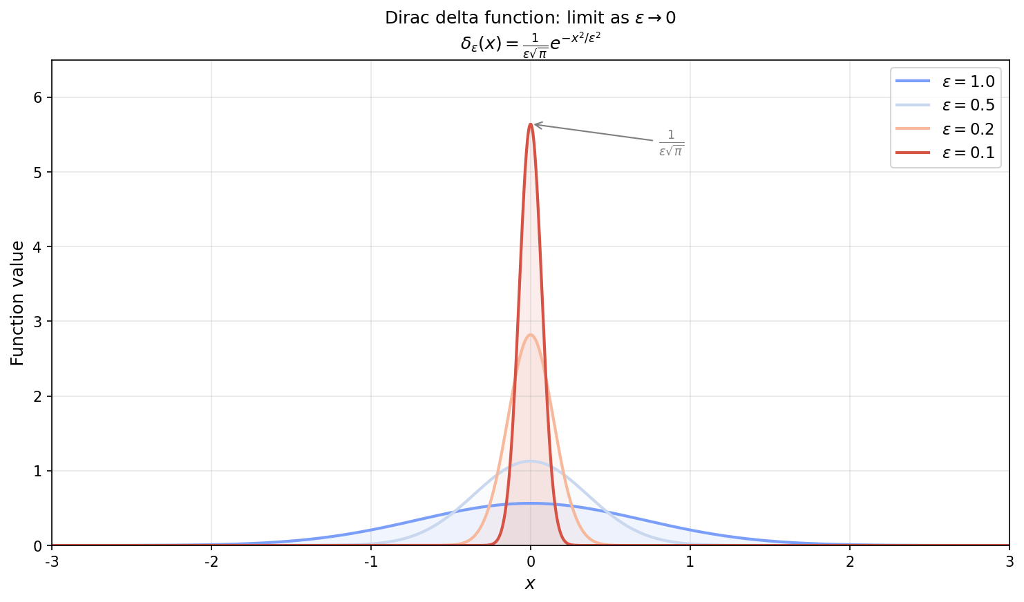
Fig. C.2: The Dirac delta function as a limit of Gaussian functions. The δ function is defined as the limit of narrowing the Gaussian width \(\epsilon\). The integral value remains 1 for all \(\epsilon\), and in the \(\epsilon\to 0\) limit it becomes a singular function that is "infinite only at \(x=0\)." A universal tool for representing "points" in physics.
🟡 Lina: Other sequences such as rectangular functions or Lorentzian functions give the same limit:
No matter which sequence you use, the limit satisfies the sifting property (C.24).
Basic Properties of the δ Function
🟡 Lina: Let me summarize the important properties of the δ function:
(1) Sifting property (restated):
(2) Even function property:
(3) Scaling:
The even function property (C.28a) can also be seen as a special case of the scaling rule (C.28b) with \(a = -1\).
(4) Composition:
Here the \(x_i\) are the simple roots of \(g(x) = 0\) — that is, roots satisfying \(g'(x_i) \neq 0\). In high school you learned about "repeated roots" of quadratic equations, right? Those were cases where the parabola is tangent to the \(x\)-axis. The same idea applies here: if \(g'(x_i) \neq 0\), the graph \(y = g(x)\) "crosses" the \(x\)-axis (simple root); if \(g'(x_i) = 0\), it merely "touches" it (repeated root). For example, \(g(x) = x^2 - 1\) has \(g'(\pm 1) = \pm 2 \neq 0\) at \(x = \pm 1\), so the graph crosses—these are simple roots. Conversely, \(g(x) = x^2\) at \(x = 0\) has \(g'(0) = 0\), and the graph only touches the axis. In such repeated-root cases, \(1/|g'(x_i)|\) diverges, so this formula cannot be used directly (a higher-order expansion is needed. In physics problems, the simple-root case is almost always what arises, so don't worry).
🔵 Kai: How do you derive this?
🟡 Lina: It can be understood as a generalization of the scaling rule (C.28b). Remember the sifting property of the δ function—\(\delta(\text{something})\) only contributes to the integral at points where "something \(= 0\)." So \(\delta(g(x))\) only contributes at points where \(g(x) = 0\), that is, at each root \(x_i\).
🔵 Kai: So only the "neighborhood" of the roots matters?
🟡 Lina: Right. When computing \(\int f(x)\,\delta(g(x))\,dx\), regions where \(g(x) \neq 0\) don't contribute because \(\delta\) is zero there. The only contributions come from the "immediate neighborhood" of each root. So we can split the integral into neighborhoods around each root: \(\int = \sum_i \int_{\text{near } x_i}\).
Near each root, we can linearly approximate \(g(x)\)—the same idea as "tangent line equations" from high school. Let's build intuition with a specific example first. For \(g(x) = x^2 - 1\), the roots are \(x = 1\) and \(x = -1\). Near \(x = 1\): \(g(x) = x^2 - 1 \approx 2(x - 1)\) (tangent slope \(g'(1) = 2\)).
⚪ Mei: Since the δ function only "sees" the immediate neighborhood of \(x = 1\), this linear approximation is sufficient.
🟡 Lina: Exactly. In general, the linear approximation of \(g(x)\) near \(x_i\) is \(g(x) \approx g(x_i) + g'(x_i)(x - x_i)\) (the same form as the tangent line equation \(y \approx y_0 + f'(x_0)(x - x_0)\) from high school). Since \(g(x_i) = 0\) (by definition of a root), we get \(g(x) \approx g'(x_i)(x - x_i)\). Why is a linear approximation sufficient? Because the δ function only picks up contributions from the immediate neighborhood of \(x_i\)—a range of nearly zero width. Within that "nearly zero width," higher-order terms \(g''(x_i)(x-x_i)^2/2 + \cdots\) are negligibly small compared to the first-order term in \((x-x_i)\), so the linear approximation suffices. Then \(\delta(g(x)) \approx \delta(g'(x_i)(x - x_i))\), and applying the scaling rule (C.28b) with \(a = g'(x_i)\) gives \(\frac{1}{|g'(x_i)|}\delta(x - x_i)\). Summing contributions from all roots gives equation (C.28c).
🔵 Kai: I see, because the δ function is a "zero-width filter," approximating as linear near the root introduces no error.
🟡 Lina: Exactly. Let's look at a concrete example. For \(\delta(x^2 - 1) = \delta((x-1)(x+1))\), we have \(g(x) = x^2 - 1\) with roots \(x = \pm 1\). Since \(g'(x) = 2x\), \(|g'(1)| = 2\) and \(|g'(-1)| = 2\). Therefore \(\delta(x^2-1) = \frac{1}{2}\delta(x-1) + \frac{1}{2}\delta(x+1)\).
⚪ Mei: Each root's contribution is weighted by \(1/|g'|\) and summed. Roots where the graph crosses more steeply contribute less—an image of the δ function's "area" being spread thinner there.
(5) Product with \(x\):
🔵 Kai: Why does equation (C.28d) hold? \(\delta(x)\) is infinite at \(x = 0\), yet multiplying by \(x\) gives zero?
🟡 Lina: As a distribution, the meaning is "the integral of \(x\,\delta(x)\) with any \(f(x)\) is zero." Thinking of \(f(x) \cdot x\) together as \(h(x) = x\,f(x)\), by the sifting property (C.24):
Since \(\delta(x)\) extracts the value at \(x = 0\), the factor \(x\) gives \(0\).
🔵 Kai: How should I intuitively understand the scaling rule (C.28b)?
🟡 Lina: \(\delta(ax)\) has its peak at \(x = 0\) just the same, but it's "compressed" by a factor of \(a\). To maintain area \(1\), the height must be multiplied by \(1/|a|\). You can verify this with the substitution \(u = ax\). Since \(du = a\,dx\), we have \(dx = du/a\). For \(a > 0\), \(u = ax\) moves in the same direction as \(x\), so when \(x: -\infty \to +\infty\), \(u: -\infty \to +\infty\) and the integration range stays the same. Substituting \(dx = du/a\): \(\int_{-\infty}^{+\infty} f(u/a)\,\delta(u)\,\frac{du}{a}\). By the sifting property (C.24), \(\delta(u)\) selects \(u = 0\), so \(f(u/a)\big|_{u=0} = f(0)\), giving \(= \frac{f(0)}{a} = \frac{f(0)}{|a|}\) (since \(a > 0\), \(a = |a|\)).
For \(a < 0\), a bit more care is needed. With \(u = ax\) and \(a < 0\), as \(x\) goes from \(-\infty\) to \(+\infty\), \(u\) goes from \(+\infty\) to \(-\infty\) (the direction reverses). Under the substitution:
Using the property of definite integrals \(\int_b^a (\cdots)\,du = -\int_a^b (\cdots)\,du\) to swap the limits: \(= -\int_{-\infty}^{+\infty}f(u/a)\,\delta(u)\,\frac{du}{a}\). Combining the prefactors gives \((-1) \times \frac{1}{a}\). Since \(a < 0\), writing \(a = -|a|\): \((-1) \times \frac{1}{a} = \frac{-1}{a} = \frac{-1}{-|a|} = \frac{1}{|a|}\). Thus:
In summary, whether \(a > 0\) or \(a < 0\), the final result is the same:
On the other hand, the integral of \(\frac{1}{|a|}\delta(x)\) with \(f(x)\) is also \(\int f(x)\cdot\frac{1}{|a|}\delta(x)\,dx = \frac{f(0)}{|a|}\). Since both match, equation (C.28b) holds.
⚪ Mei: I see—the scaling rule is consistent between the intuition "compressing changes the height to preserve area" and the variable-substitution calculation.
Derivative of the δ Function
🟡 Lina: The "derivative" \(\delta'(x)\) of the δ function can also be defined. In integration-by-parts form:
🔵 Kai: When you differentiate, it extracts not the value of \(f\) but the derivative of \(f\). The minus sign is from integration by parts?
🟡 Lina: Yes. Formally integrating by parts:
The boundary term vanishes because \(\delta\) is zero at infinity.
✅ Comprehension Check: Compute \(\int_{-\infty}^{\infty}(3x^2 + 2x - 1)\,\delta(x - 2)\,dx\).
Answer
By the sifting property: \(f(2) = 3(4) + 2(2) - 1 = 12 + 4 - 1 = 15\).
📝 Exercises:
- Compute \(\int_{-\infty}^{\infty}e^{-x^2}\,\delta'(x)\,dx\) → Problem B-7. Evaluate the following integral using the Fourier integral representation of the δ function (Eq. (C.19))
C.7 The δ Function as a Sum over Complete Sets — Fourier Integral Representation and the Discrete Basis Case
🟡 Lina: Finally, let's look at the deep relationship between the δ function and "complete sets." This is the most frequently used form of the δ function in quantum mechanics.
Fourier Integral Representation
🟡 Lina: We already used this in equation (C.19), but let me derive it properly now. Substituting equation (C.16) into the inverse Fourier transform (C.17):
Interchanging the integration order and rearranging:
For this equation to hold for arbitrary \(f(x)\), the expression in brackets must be \(\delta(x - x')\). Therefore:
🔵 Kai: The δ function is "the sum of all plane waves with equal weight at every wavenumber"!?
🟡 Lina: Yes! Intuitively, \(e^{ik(x-x')}\) is always \(1\) at \(x = x'\), so all waves constructively interfere. At \(x \neq x'\), the phases are random and cancel out. The result is a sharp peak only at \(x = x'\).
🔵 Kai: Is that the same principle as interference in the double-slit experiment? Constructive interference where phases align, destructive where they don't.
🟡 Lina: Beautiful analogy. The double slit involves interference of 2 waves, but here infinitely many plane waves are interfering. The principle is the same: "if phases align they reinforce, if random they cancel." You can think of the δ function as the ultimate interference of infinitely many slits. Let's verify with equations. At \(x = x'\): \(e^{ik(x-x')} = e^0 = 1\), so the integrand is constant \(1\), and the integral over infinite range in \(k\) diverges—this is the "infinite peak." At \(x \neq x'\): \(e^{ik(x-x')}\) oscillates in \(k\), so cancellation occurs giving zero. Indeed, the δ function's property of being "nonzero only at \(x = x'\)" is reproduced.
⚪ Mei: So at \(x = x'\) where phases align, all waves constructively interfere and diverge, while at \(x \neq x'\) where phases are random, they cancel to zero—Lina's intuitive explanation is directly expressed in the equations.
🟡 Lina: Exactly. Equation (C.30) is called the Fourier integral representation of the δ function and is used everywhere in quantum mechanics.
The Discrete Basis Case — Completeness Relation
🟡 Lina: Not just the continuous basis \(\{e^{ikx}\}\), but the same structure appears for discrete orthonormal bases \(\{\phi_n(x)\}\) as well.
As you learned in Appendix B, if there exists a complete orthonormal basis \(\{\phi_n(x)\}\), any function can be expanded:
(The integration range is the entire domain where the function is defined. For all space it's \((-\infty, \infty)\); for a finite interval \([0, a]\), it's that interval. The same domain is used for integration in the equations below.)
Substituting \(c_n\) (the integration variable in \(c_n\) is \(x'\), separate from the expansion variable \(x\)):
Writing out each term: \(\sum_n \phi_n(x)\int \phi_n(x')^*\,f(x')\,dx'\). Since \(\phi_n(x)\) doesn't depend on \(x'\), it can be brought inside the integral: \(\sum_n \int \phi_n(x)\,\phi_n(x')^*\,f(x')\,dx'\). Furthermore, interchanging the sum and integral:
🔵 Kai: Ah, \(f(x')\) has been factored out, and the bracket contains "only basis information."
🟡 Lina: Right. In the second equality, we interchanged the sum and integral and factored out \(f(x')\). In Section C.5 I explained interchanging the order of integrals, and here it's interchanging an "infinite sum" and an "integral." The idea is the same—summing each term \(\phi_n(x)\int\phi_n(x')^*f(x')\,dx'\) and first forming \(\sum_n \phi_n(x)\phi_n(x')^*\) then integrating over \(x'\) give the same result for sufficiently well-behaved functions. Since this holds for arbitrary \(f(x)\):
🔵 Kai: The "completeness" of an orthonormal basis is expressed by the δ function!
🟡 Lina: Yes. Equation (C.31) is called the completeness relation. "The basis is complete" means precisely that this equation holds.
Concrete Example: Eigenfunctions of the Infinite Well
🟡 Lina: Let's look at a concrete example. As an orthonormal basis for expanding functions defined on the interval \([0, a]\) that vanish at both endpoints (\(f(0) = f(a) = 0\)):
These are also the eigenfunctions of the "infinite square well potential" that you'll learn later, but for now just think of them as "an orthonormal complete set on the interval \([0, a]\)." The completeness relation holds:
⚪ Mei: The continuous version (C.30) and the discrete version (C.32) both have the same structure: "summing over all basis functions gives the δ function."
🟡 Lina: Exactly. In quantum mechanics:
- Continuous spectrum (free particle momentum eigenstates, etc.) → equation (C.30) type
- Discrete spectrum (bound state energy eigenstates, etc.) → equation (C.31) type
These are the two faces of "completeness." When you learn Dirac notation in Ch. 11, these can be written in a unified way as:
🔵 Kai: What are \(|\phi_n\rangle\) and \(\langle\phi_n|\)? Is it just equation (C.31) rewritten in different notation?
🟡 Lina: Good intuition. Exactly. Writing \(\phi_n(x)\) as \(|\phi_n\rangle\) and \(\phi_n(x')^*\) as \(\langle\phi_n|\) is Dirac notation. You'll learn it in detail in Ch. 11, so for now just know that "there exists a convenient notation that unifies discrete and continuous cases."
🔵 Kai: I see, so it's just equation (C.31) in different notation. But one thing I'm curious about—for the continuous case \(\int |k\rangle\langle k|\,dk\), what about the "inner product" between \(|k\rangle\)'s? In the discrete case there was orthonormality \(\int \phi_m(x)^* \phi_n(x)\,dx = \delta_{mn}\), but what happens in the continuous case...
🟡 Lina: Sharp question. In the continuous case, \(\langle k|k'\rangle = \delta(k - k')\)—the Kronecker delta gets replaced by the Dirac δ function. But this is material for Ch. 11, so for now just keep in the back of your mind that "such an extension exists."
🔵 Kai: Ah, so in the discrete case it's \(\delta_{mn}\) and in the continuous case it's \(\delta(k - k')\). I'd been wondering why they're both called "delta"—so one is the continuous version of the other. But \(\delta_{mn}\) takes finite values "0 or 1," while \(\delta(k-k')\) is "infinity or zero." They look completely different, yet serve the same role—that's strange...
🟡 Lina: Good question. The key is "what you combine them with." \(\delta_{mn}\) is combined with a sum \(\sum_n\) to select one term: \(\sum_n c_n \delta_{mn} = c_m\). \(\delta(k-k')\) is combined with an integral \(\int dk'\) to select one point: \(\int \tilde{f}(k')\delta(k-k')\,dk' = \tilde{f}(k)\). In the discrete case, a value of \(1\) suffices to "select one term," but in the continuous case, infinite height is needed to "select one point"—since an integral is "width × height," to get a finite contribution from a point of zero width requires infinite height.
⚪ Mei: The same pattern of discrete sums becoming continuous integrals also appears in the expression of orthogonality. Using \(\cos\) orthogonality to "extract" Fourier coefficients in Section C.1, and the δ function "selecting" \(k' = k\) in Section C.4—they're all the same principle: "taking the inner product with orthogonal basis elements leaves only one." The discrete and continuous versions of this.
🟡 Lina: Right. Think of the Kronecker delta being "promoted" to the Dirac delta. The transition from discrete to continuous appears consistently in both basis expansions and orthogonality expressions.
Other Integral Representations of the δ Function
🟡 Lina: Finally, let me list some commonly used integral representations of the δ function besides equation (C.30):
(1) Fourier integral representation (restated):
(2) Representation via the sinc function:
(3) Representation from Fourier series (period \(L\)):
The right-hand side is actually a function with period \(L\), having δ function peaks at \(x = 0, \pm L, \pm 2L, \ldots\). Restricting to \(|x| < L/2\) includes only the peak at \(x = 0\), so within that range it coincides with \(\delta(x)\).
🔵 Kai: Is equation (C.34) the integral in equation (C.33) truncated to the finite range \([-N, N]\)?
🟡 Lina: Exactly!
This converges to the δ function as \(N \to \infty\).
🔵 Kai: Does equation (C.35) really satisfy the sifting property too? How would you verify that...
🟡 Lina: Good question. The verification method is the same as before—multiply both sides by \(f(x)\) and integrate. Let's actually do it. Multiplying both sides of (C.35) by \(f(x)\) and integrating from \(-L/2\) to \(L/2\): the left side by the sifting property gives \(\int_{-L/2}^{L/2} \delta(x) f(x)\,dx = f(0)\). The right side becomes \(\frac{1}{L}\sum_n \int_{-L/2}^{L/2} f(x)\,e^{i\frac{2\pi n}{L}x}\,dx\).
⚪ Mei: The right side's \(\int_{-L/2}^{L/2} f(x)\,e^{i\frac{2\pi n}{L}x}\,dx\) looks similar to \(c_n\) from equation (C.11), but with the opposite sign in the exponent.
🟡 Lina: Good observation. Recalling equation (C.11): \(c_n = \frac{1}{L}\int f(x)\,e^{-ik_n x}\,dx\). Replacing \(n\) with \(-n\): \(c_{-n} = \frac{1}{L}\int f(x)\,e^{+ik_n x}\,dx\). Each term on the right, \(\frac{1}{L}\int f(x)\,e^{i\frac{2\pi n}{L}x}\,dx\), is exactly \(c_{-n}\). So the right side is \(\sum_{n=-\infty}^{\infty} c_{-n}\). But since the summation range is \(-\infty\) to \(+\infty\), replacing \(n\) with \(-n\) doesn't change the range. Therefore \(\sum_{n=-\infty}^{\infty} c_{-n} = \sum_{n=-\infty}^{\infty} c_n\). Meanwhile, setting \(x = 0\) in equation (C.10) gives \(f(0) = \sum_{n=-\infty}^{\infty} c_n\). So the right side also equals \(f(0)\). Everything is consistent.
🔵 Kai: Since the summation range is symmetric from \(-\infty\) to \(+\infty\), relabeling \(n\) changes nothing. Makes sense.
✅ Comprehension Check: State the physical meaning of the completeness relation \(\sum_n \phi_n(x)\phi_n(x')^* = \delta(x-x')\).
Answer
It means that the basis \(\{\phi_n\}\) is "complete"—that any function can be expanded in this basis. If the basis were incomplete (some \(\phi_n\) missing), the sum would not equal \(\delta(x-x')\), meaning there would exist functions that cannot be represented by the expansion.
📝 Exercises:
- Plot \(\frac{\sin(Nx)}{\pi x}\) for \(N = 5, 20, 100\) in equation (C.34) and confirm that it approaches the δ function as \(N\) increases → Problem M-4. Fourier Integral Representation of the δ Function
Summary — Formula List for This Chapter
🟡 Lina: Finally, here's a summary list of the main formulas introduced in this Appendix. Come back here for reference whenever you need them in the main text.
Table C.2: Summary of main formulas in Appendix C
| Name | Formula | Eq. No. |
|---|---|---|
| Fourier series (real form) | \(f(x) = \frac{a_0}{2} + \sum_{n=1}^{\infty}\left[a_n\cos\!\left(\frac{2\pi n}{L}x\right) + b_n\sin\!\left(\frac{2\pi n}{L}x\right)\right]\) | (C.5) |
| Complex Fourier series | \(f(x) = \sum_{n=-\infty}^{\infty}c_n\,e^{ik_n x}\) | (C.10) |
| Fourier transform (symmetric convention) | \(\tilde{f}(k) = \frac{1}{\sqrt{2\pi}}\int f(x)\,e^{-ikx}\,dx\) | (C.16) |
| Inverse Fourier transform | \(f(x) = \frac{1}{\sqrt{2\pi}}\int \tilde{f}(k)\,e^{ikx}\,dk\) | (C.17) |
| Parseval's equality | \(\int\lvert f(x)\rvert^2\,dx = \int\lvert \tilde{f}(k)\rvert^2\,dk\) | (C.18) |
| Convolution theorem | \(\widetilde{(f*g)}(k) = \sqrt{2\pi}\,\tilde{f}(k)\,\tilde{g}(k)\) | (C.22) |
| Sifting property of δ function | \(\int f(x)\,\delta(x-a)\,dx = f(a)\) | (C.24) |
| Fourier representation of δ function | \(\delta(x) = \frac{1}{2\pi}\int e^{ikx}\,dk\) | (C.33) |
| Completeness relation (discrete) | \(\sum_n \phi_n(x)\,\phi_n(x')^* = \delta(x-x')\) | (C.31) |
Preview of Next Chapter
🟡 Lina: In this chapter, we organized the mathematics of "continuous basis expansion"—Fourier analysis and the δ function. In the next chapter, Appendix D, we'll cover Lagrangian and Hamiltonian formalism and canonical quantization. Starting from the variational principle of classical mechanics, we'll see where the quantization prescription of "replacing coordinates and momenta with operators" comes from.
🔵 Kai: The "principle of least action" in mechanics connects to quantum mechanics?
🟡 Lina: Yes. The structure of Hamilton's canonical equations naturally leads to the commutation relation \([\hat{x}, \hat{p}] = i\hbar\) of quantum mechanics. The "origin" of the commutation relation introduced without derivation in Ch. 8 will naturally emerge from the Poisson brackets of classical mechanics.
⚪ Mei: The connection point between classical mechanics and quantum mechanics. Looking forward to it.
Practice Problems
📝 Exercises:
- Find the Fourier coefficients \(a_n, b_n\) for \(f(x) = x\) on the interval \([0, L]\) → Problem M-1. Find the Fourier coefficients and of the function defined on the interval , and write down the Fourier series (Equation (C.5
- Compute the Fourier transform of the Gaussian function \(f(x) = e^{-ax^2}\) (\(a > 0\)) → Problem M-2. Fourier Transform of a Gaussian Function and Parseval's Theorem
- Plot \(\frac{\sin(Nx)}{\pi x}\) for \(N = 5, 20, 100\) in equation (C.34) and confirm that it approaches the δ function as \(N\) increases → Problem M-4. Fourier Integral Representation of the δ Function
- Show that the Fourier transform of \(f'(x)\) is \(ik\tilde{f}(k)\) (use integration by parts) → Problem M-5. Differentiation Property of the Fourier Transform
- Compute \(\int_{-\infty}^{\infty}e^{-x^2}\,\delta'(x)\,dx\) → Problem B-7. Evaluate the following integral using the Fourier integral representation of the δ function (Eq. (C.19))
References
- Katsuhiko Hiroe, Quantum Mechanics as a Hobby — Chapter 5, "Fourier Analysis." Referenced for the flow of derivation from Fourier series to Fourier transform, and the discussion of the δ function's Fourier series expansion.
- D. J. Griffiths, Introduction to Quantum Mechanics, 3rd ed. — Referenced for the free particle and wave packet discussions in Chs. 2–3, and the organization of δ function properties in the treatment of the δ function potential.
Feedback on this page
Let us know if something was unclear, incorrect, or could be improved.